Demand planning in excel

When it comes to visualizing data in the S&OP process, most stakeholders like to see forecasting outputs in the form that they are most familiar with – Excel. This is certainly true in my experience working in global FMCG companies.

Below I present an Excel tool which I have used many times as a Demand Planner. What you see below has been employed at the Demand Review meetings to great effect at large corporations with very mature demand planning and S&OP processes. It is an ideal solution both for smaller companies just starting their S&OP process that do not want to make a big investment in technology, as well as bigger companies where stakeholders want an easy to understand and recognizable format of data presentation.

Click Here To Download The Forecasting Demand Review Tool

It opens in the web version of Excel. I recommend to download to your computer and open in the Excel application. You can input your own data into this tool from an advanced system (e.g. statistical forecast from APO).

Purpose Of The Tool

The purpose of the tool is too support discussion at the Demand Review meeting with data in format familiar to all stakeholders, and with analytical functionalities that will help to finish the meeting with best possible consensus forecast, including incorporating information from Sales.

As the meeting involves many departments including Demand Planning, Sales , Marketing and Finance, the goal is not to review forecasts SKU by SKU, but on an aggregated level. The level of aggregation depends on the product complexity, i.e. the number of categories/brands/SKU’s. Discussion should be had for groups of products with similar sales characteristics, e.g. groups of products that are sold in similar percent splits. Further volume split per SKU can be determined by more or less advanced statistical methods.

View & Functionalities

The tool operates on historical sales data and forecast figures. Data are presented on different level of aggregation. For product dimension, the tool presents historical sales data and forecast at three aggregation levels: product group/segment/category. For the customer dimension, there are also 3 aggregation levels at which the user can review historical sales: customer/channel/market.

Selection and historical data:

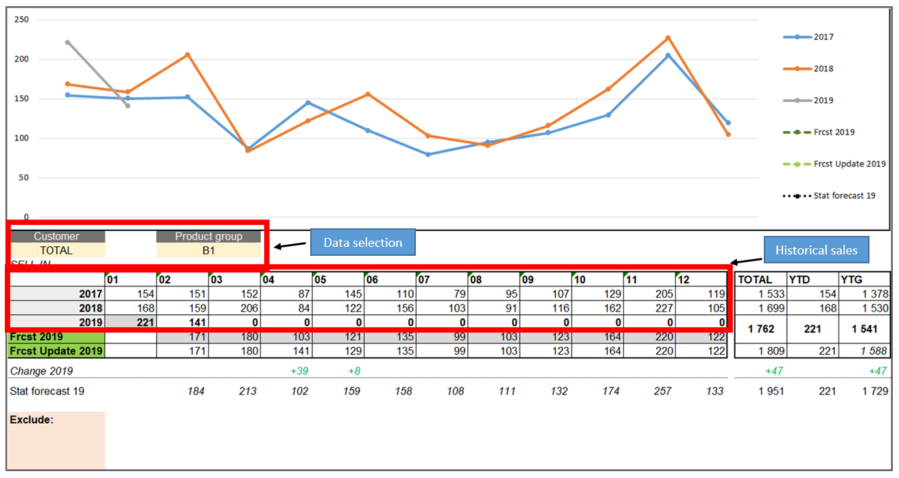
The above screenshot shows customer and product data. The user can select historical sales data and forecast of Product Group A. It is possible to drill down to sales of Product Group A for particular a customer or sales channel. The tool shows the current and previous two years of sales. The reason I choose 2 previous years of sales is that when looking at the chart it is quite easy to understand the seasonality of the product.

Forecast data: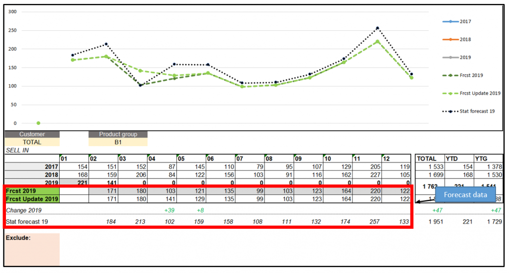On the above screenshot you can see forecast data from the last cycle, labelled “Frcst 2019”, then below, you can see the new figures which were updated in the meeting. The user simply types new figures in this line at the lowest level of Product dimension (Product Group) and saves them. The next line “Change 2019” shows the differences between the updated and last cycle figures. The line “Stat forecast 19” is a Seasonal+Linear regression model that is built in Excel and calculates a statistical forecast based on historical sales in the current selection.

The user has the possibility to select what kind of data lines he/she would like to see on the chart through check boxes.

Exclude customers functionality:

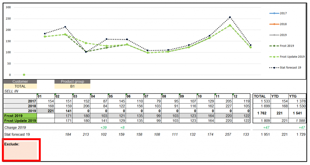
The functionality in the red box in the above screenshot allows users to exclude particular customers simply by pasting their name into the pink area. It is useful when we want to look at overall market sales without customers that cause outlying sales. These volatile customers can skew our view of the whole market.

How To Use The Demand Review Tool

Usually, a more detailed customer forecast revision is done for the period which is going to be frozen in current S&OP/IBP cycle. Demand review and analysis of the forecast for this particular month can be structured in the following way:

Forecast analysis on product group level for frozen month:

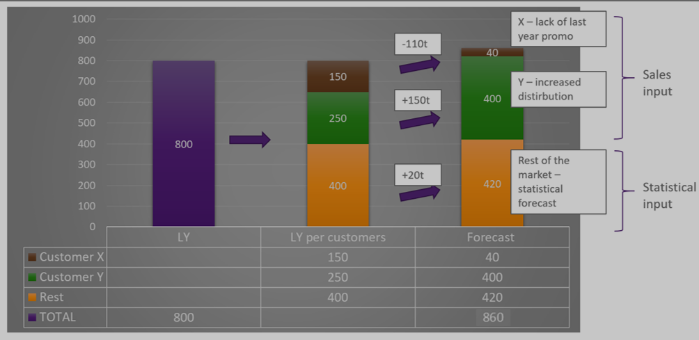
• The starting point for analysis can be last year’s figures (naïve forecast)
• Creation of building blocks – separation of 2 or 3 top customers with biggest events (in analogical period LY or planned for future) and rest of the market
• Revision and agreement on the forecast for each building block
• Aggregation of figures

Such an approach differs from the standard approach where segmentation is done according to product dimension. This higher-level approach can help Demand Planners to speak the same language as the Sales team which is oriented towards activities per customer. We can imagine a team of Key Account Managers and each of them comes to the meeting sharing details about their customer/channel. The above tool can be very useful in consolidating their input and challenging it with data (historical sales or statistical forecast).

Another benefit of the tool is easier estimation of promo uplift for particular customers (e.g. by finding periods of similar promotion in data). It is impossible to judge promo impact of a particular customer looking at data for whole market. Of course, the alternative is to deep dive into sales reports per customers.

High-Level Demand Review Process Steps

• Sales to prepare info of upcoming events by customer that will impact sales and prepare info about marketing campaigns/events
• Demand planning to analyze historical data, especially for focus month and recent trends
• Reviewing most important/volatile SKU’s.
• Revision of the forecast by product groups (see chart above) and agreement on final figures

The role of Demand Planning is to work out the optimum SKU mix. Commercial teams should not be involved in forecast revision SKU by SKU. However, if they are aware about events concerning single SKUs (e.g. recommendation at the cashier or new listing), the Demand Review meeting is the right place to deliver such information.

Summary

People and the underlying process are the foundation of effective S&OP, especially for companies that are just starting to implement it. This Excel tool can be a great support to start your S&OP journey. After building process maturity, investment in advanced systems can provide further results.

Analytics for demand planning in Excel usually involves big tables of data.  To understand the demand for a product, you need to look into its history.  Analytics with an order history over a year or more can have 100K+  records.  Here is a technique to perform fast analytical formulas on many thousand rows.

The order history will come out of a transaction system, usually MRP / ERP.  Each order record is a single order for a product, so it is a raw, lumpy transaction history.  It is helpful to smooth this demand out, so a common analytics calculation is the rolling average.  A rolling average over n days is much better than a weekly or monthly average and allows demand planners to calculate a service level for every part.

The easiest way to calculate this using the Excel AVERAGE formula across a fixed range of cells that represents the rolling average period.  The problem with this method is that it requires your order history to have zero values for non-order days.  After all, in our analysis we want to know what the average demand is for all days (calendar or working) not just the days that happen to have orders for that product.

Furthermore, the order date is not necessarily the most relevant date.  A much better date is usually the due-date or commit-date when the order should ship out.  So, combining the order book with all those extra date records is not practical.

In analytics for demand planning, we want to calculate rolling averages and service levels for every product, on every order day.  This requires single formula that we can apply to the order history and see how smoothed demand changes over time.

It looks like this formula will involve SUMIF and COUNTIF.  More precisely, multiple condition SUMIFs and COUNTIFs for the product code and date ranges.  Excel 2007 has SUMIFS, COUNTIFS formula and those on Excel 2003 can use SUMPRODUCT or  SUM(IF…) array formulas.

The trouble is that SUMIF is a very calculation intensive formula.  Just try and paste a SUMIF formula to every row in a table with 10K+ rows and see how long it takes.  We can avoid doing SUMIF (and COUNTIF etc) on a long criteria range by sorting first.

Excel sorts very fast.  You can sort a table of demand data by product code and date in an instant.  You have the choice to use a pivot table or Data|Sort command in the menu ribbon or bar.  The sorted range can then be identified using the first row and last row numbers.  The first and last row for a continuous list of product codes is a replacement for putting the product code as a criteria.   This makes your criteria ranges much smaller and the formula calculation much faster.

Download a demand analytics example of this and you can see exactly how it works.  This has a simple rolling average analysis for demand history with 65K rows to make it compatible with Excel 2003.

The data originally came from a text file import with ItemCode, Qty, OrderDate and CommitDate fields.  The data connection link is not live in this example, but you can easily set it up for the original file, or add your own demand history using text files to connect with system data.

After refreshing the demand data, hit the “Update” button on the Orders sheet.  The first thing that the macro does is sort the demand history data by ItemCode and CommitDate.  This puts all of the ItemCodes in a continuous range and the dates in chronological order.  The next step is to paste down the formulas that calculate first and last row number for each ItemCode range.  We will use this to specify a range that covers each block of ItemCode records.

This demand analytics example is created with the Fast Excel Development Template which is a free download and contains many useful functions for setting formulas once and applying them to thousands of records at the click of a button.  We use the template to build of planning and scheduling systems, and demand planning is an increasingly popular application.  There are some template video tutorials here to get you up and running with the template.  The Sort function, dynamic named ranges and mutiple paste downs are covered in the Query Template Tutorial.

Back to the demand analytics example.  You can specify a range using the first row and last row numbers using INDEX, INDIRECT or OFFSET.  I prefer to use INDEX as below

INDEX(DateRange,ItemFirstRow):INDEX(DateRange,ItemLastRow)

eg.  INDEX($E:$E,$G11):INDEX($E$E,$H11)

Now the range for the SUMIFS is only as high as the number of records for that particular part.  This makes the calculation much faster.  The actual rolling average formula is like so:

SUMPRODUCT(–(INDEX($E:$E,$G11):INDEX($E:$E,$H11)>$E11-I$6),–(INDEX($E:$E,$G11):INDEX($E:$E,$H11)<=$E11),INDEX($B:$B,$G11):INDEX($B:$B,$H11))/I$6

Where cell I6 holds the number of days in the rolling average period.

Once you have a rolling average value over time, you can apply a service level to each record.  This means that demand planners can work out what is the average daily demand for the periods where it has been the highest.   Here is a more detailed discussion of demand analytics, rolling averages and service levels.

Use this technique to measure demand variation, order frequency over the entire order history.  These are valuable metrics to use to analyze the pattern of orders and understand some key characteristics that help us predict how demand will change in the future.

Do you need an all-in-one tool to plan future demand for your products? Then, this Sales Forecast Excel Template will help you forecast your future revenue according to your historical sales data.

Above all, this tool has the advantage to work in the same way as the forecasting module. Because it has the versatility to add new SKUs (Stock Keeping Unit) with their own automatic code number created and calculate Sales Forecast according to Holt-Winter’s Exponential Smoothing Method.

This Sales Forecasting Template will help you to calculate your sales according to the corrected historical data monthly. It’s just like how ERP systems work.

With this tool, you have the chance to calculate and release your sales forecasting. Here is what you can do:

• You can add or create new products in a simple Sales History Data Worksheet with an automatic code number for each SKU.
• For mature products, you can also upload your corrected sales history data in the related Worksheet.
• In Set Forecast Worksheet, you can calculate your sales forecast by changing the statistical constants: Level, Trend, and Seasonality according to your knowledge as a demand planner to reduce MAPE (Mean Average Percentage Error).
• You can adjust your final forecast on a quarterly basis by watching changes in the dynamic

SALES FORECAST EXCEL TEMPLATE MAIN FEATURES

Basically, this Excel template consists of 3 main parts:

Now, let’s check the three main sections of our Sales Forecasting Template:

1. Sales History

In this sheet, you can add or create new products by filling the blank fields. In this case, new products must be forecasted under expected sales assumptions according to Min. Expected Sales and Max. Expected Sales which represents our sales history basis.

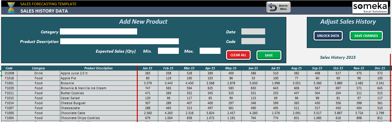
This section works as a simple Master Data setting up an automatic code when you save your new product. As Master Data of this demand planning template, statistical constants for Level, Trend, and Seasonality will take 0.3 as the default value.

You will be able to change these values when you execute the sales forecast for each new product. Other constants for quarter adjustments on the final forecast are going to be set up on 100% as the default value; you can also change these values on forecast execution.

In case you have Mature Products as data coming from another system, you can also import this data by pressing the UNLOCK DATA button and fields will be unlocked to paste your own Sales History Data.

We recommend at least 4 years of corrected history in this template for accurate demand planning and sales forecasting. In case you don’t have enough sales history, we recommend you complete missing values with the moving average.

Warning!: Do not input zero values as sales history; in that case, complete the sales history with the moving average. Save your input data by pressing the SAVE CHANGES button.

Finally, for uploaded mature products, you should set up the values of the statistical: Level, Trend, Seasonality, and Quarter Adjustments on 100% in the Final Forecast worksheet.

2. Set Forecast (Winter’s Exponential Smoothing)

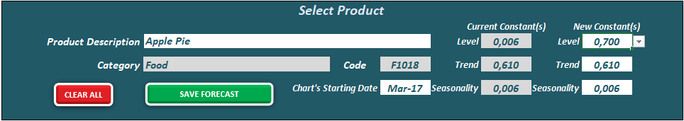
In this section, you are going to be able to run and calculate your Sales Forecast. The only thing you have to do is select any product from the object list.

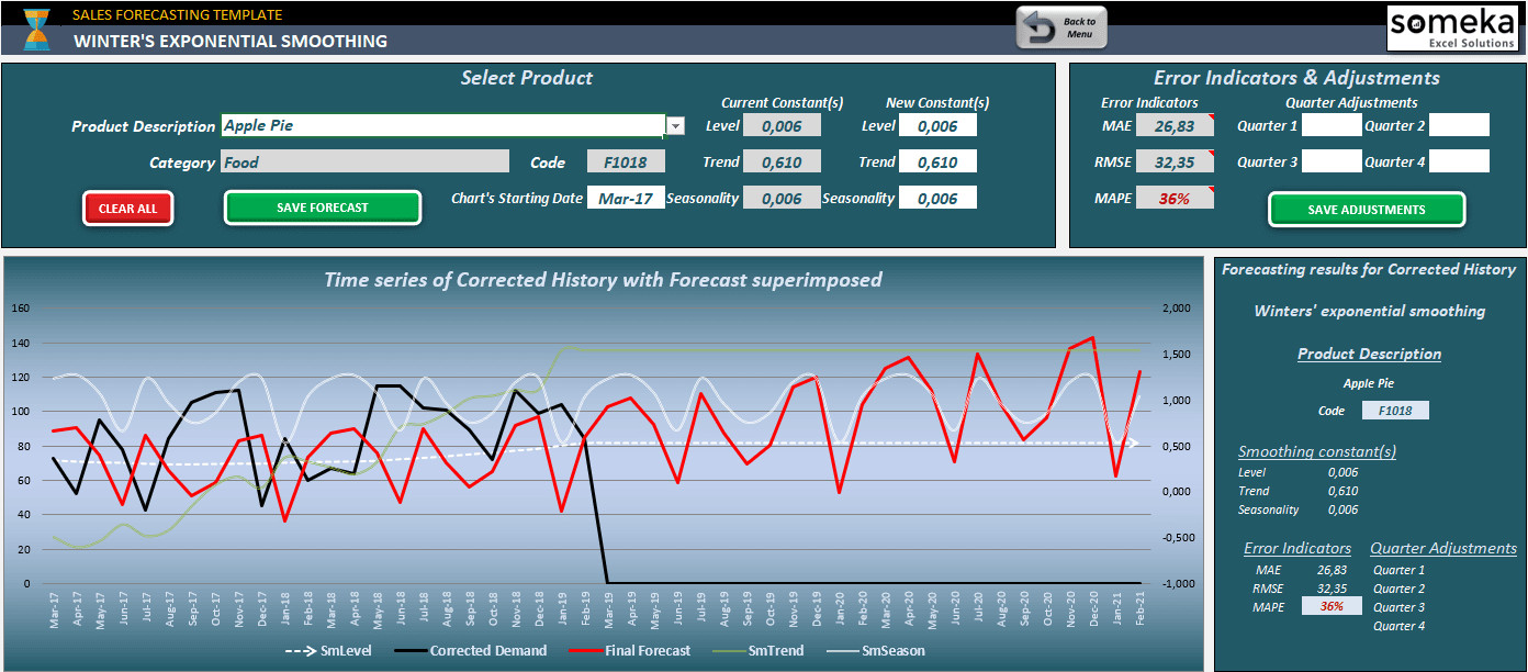
After that the default constant values will appear on the Current Constant(s) fields; now you are able to change statistical constant values: Level, Trend, and Seasonality on the right side-scrolling at the object list with values between 0,001 and 1,000.

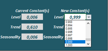
Dynamic Chart will change automatically. On this demand planning template, we recommend lower values to cover corrected history as much as possible and get a more accurate forecast reducing MAPE (Mean Average Percentage Error).

**Take into account the constant values close to 1,000 which will set your calculation as a Naive Forecast.

Furthermore, as a Demand Planning tool, you may know special promotions lead by marketing colleagues or  some fluctuations in market share; in this case, you are able to adjust your calculated forecast on a quarterly basis with the final sales forecast on the right side of “Error Indicators & Adjustments”

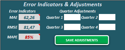
Finally, do not forget to save your sales forecast by pressing the “SAVE FORECAST” button.

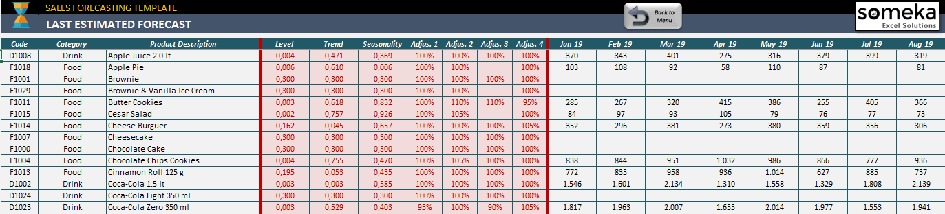
3. Final Forecast (Last Estimated Forecast)

In the last section of the Sales Forecasting Template, you will see your forecast values after saving your executed forecast. Your new forecast is now 48 months sales forecast on the planning horizon. And you will be able to change it anytime you want. Just get back Navigation Menu and press the “Set Forecast” button.

Finally, do not forget to update your real sales according to section “SALES HISTORY DATA” at the beginning of each month. Updating your real sales history will be your basis to run the next Sales Forecast with your new Sales Forecasting tool.

SALES FORECAST EXCEL TEMPLATE FEATURES SUMMARY:

• Unique Excel template to perform Sales Forecast by SKU
• Works on Windows
• Ready-to-use Sales Forecasting
• No installations needed
• Dynamic Charts
• Compatible with Excel 2007 and later versions

Gartner estimates that by 2020, 60% of revenue in supply chain dependent industries will be driven by digital business. What this essentially denotes is that the congruence of people, business, and process (or things), is ever-looming.

Image by: Arkieva

Okay, let’s be honest. This is not a new concept.

Most businesses today, employ some degree of IT data management or automation to eliminate manual processes and are heavily invested in creating a digital supply chain. For manufacturing businesses, successful companies consistently strike the right balance between customer demand and supply planning through the meticulous implementation of internal and external processes and systems.

They leverage the power of planning, collaboration, communication, market intelligence, decision-making, and risk mitigation. The decision-making and planning without the right technology solutions leaves businesses without the actionable insights needed to stay ahead of the curve. 

Read More: The ABCDs of an Excellent Supply Chain

Irrespective of the scale of business, companies need to regularly review their processes and systems and decide the most suitable tools and applications to cater to their business requirements. Here’s where Excel comes in.

Versatility of Excel in business world applications

Excel spreadsheets have become an integral part of most businesses across the world, irrespective of geographical location or the nature of the business. Most computers and smartphones are pre-loaded with Excel, which makes it one of the most accessible application across the globe. Excel is widely used for data entry, basic calculations, data sorting and analysis, creating forms and questionnaires, presentations, creating graphs and charts, budgeting and accounting, planning and scheduling, etc.

Excel has an excellent user-friendly interface and its basic functions are easy to learn. There is plenty of online and offline self-help material available for learning Excel. Representing data tables in graphs and charts is quick and easy. Advanced users can exploit the higher functionalities of Excel like rule-based formulas, conditional formatting, pivot tables, macros, etc.

Dynamic nature of Demand Planning

Demand Planning process generates demand forecasts based on various historical data and relevant business information. Historical data and statistical analysis are used to develop long-range estimates of expected demand. Demand Planning also analyzes the impact of marketing promotions, new product launches, and other business plans. Pricing discounts, rebates, market intelligence, and product discontinuations are also considered.

Read More: Using Excel for Planning – 4 Telltale Signs That You’ve Pushed Excel to The Limits

In today’s world, demand signals are dynamic and complex in nature due to multiple SKUs, wide distribution networks, multiple point of sales, varying geographical locations, customer demographics and seasonality. Huge amount of diverse and complex data is generated which needs to be effectively and efficiently considered in the Demand Planning process.

Normally, there are multiple Demand Planners that contribute to the Demand Planning process. There are individual Demand Planners for specific product categories, geographical regions and customer segmentation. Different inputs from these Demand Planners contribute to the overall Demand Planning process. This is where Excel starts to become limiting.

Limitations of Excel in Demand Planning Process

Excel is a great productivity tool and an excellent stand-alone business analytics and reporting tool. However, it has its own limitations which impede its effective implementation in the Demand Planning process. Excel is not designed for online collaborative work. A single Excel file can be edited by only one user at a time, which becomes time consuming for inputs by multiple users.

Merging multiple Excel files into a consolidated file is a difficult, time consuming task and is prone to inconsistency, errors and misreporting. The higher the volume of data in an Excel file, the slower the file size will process, leading to more chances for the data to get corrupt. Excel spreadsheets are also prone to human data entry errors and are vulnerable to deliberate manipulations due to inherent lack of controls. Excel is incapable of supporting quick decision making since the data might be outdated and inaccurate. It can also be very time consuming in getting the most up to date information from multiple users and summarizing the information for making business decisions.

Considerations for Demand Planning Managers

While Excel is a good tool for Demand Planning of limited SKUs with fairly steady demand and regional distribution; a Demand Planning Manager needs to evaluate the future business expansion plans, new product launches, new region expansion and marketing plans. In such a scenario, the existing Excel based Demand Planning process might not be able to handle the volume of data, scalability and running what-if scenarios for quick decision making.

Read More: Outgrowing Excel? Here’s How to Create a Centralized Demand Planning Process

Even without the need for flexible demand planning tool, one of the biggest risks that businesses face when managing planning data in Excel is often centered on the inability to transfer knowledge easily. In most business cases, there is often a “power user” who is highly versed on how every cell calculates, and the formulas being used. This type of planning process is often not scalable, leaves many businesses scrambling when their star Excel user is unavailable. In the end, Excel is great tool. In fact, most supply chain planning solutions like Arkieva adopt an Excel look and feel to make user adoption easy. It’s core limitations lie in the inability to the data redundancy, live data integration consistency, sharing and seamless collaboration needed for today’s digital business.

Enjoyed this post? Subscribe or follow Arkieva on Linkedin, Twitter, and Facebook for blog updates

Hi All

SAP has come up with a add-in for excel in 2014. All the  documentation is available in the link SAP Advanced Planning and Optimization, Demand Planning Add-In for Microsoft Excel 1.0 – SAP Help Portal Page

Kindly go though the  “Administrator’s Guide” and the “Application Help” ( market place log in needed ) .The below blog is just additional screen shots /tips /tricks/ which may help consultants.The screen shots are from a test system and for actual system the security aspects like firewall settings ,HTTPS should be considered.

The excel add in will work only on SCM7.0 EHP3 and on higher versions of EHP2.At the client side it supports Office 2010 and higher as explained in the guide

1.Open the transaction SICF. The Maintain service screen opens.

2.Click the Execute button or press F8.

3.Expand default_host in the service list.

4.Expand sap -> scmapo -> rest-> epm.

5.Double-click demand_plan_srv. The Create/Change a Service screen opens.

This is only available in  SCM7.0 EHP3 and on higher versions of EHP2 ( please refer the guide )

6.If the service is active, you can see Service (Active) written next to the service name. If you cannot see this text displayed, continue with the next step.

7.Click the Back button.

8.Right-click demand_plan_srv in the service list.

9.Select Activate Service from the context menu that appears.

10.Choose Yes in the dialog box that opens.

Now test the service

.A new window should open with a logon screen

The Url will be in the format http://[host]:[port]/sap/scmapo/rest/epm/demand_plan_srv/

If the window does not appear then few ICM setting are missing in RZ10 and this has to be checked by Basis team

The three ICM seting are shown below

At the client side

The excel add in  available  in marketplace and download access will be needed to get this file. It has multiple prerequisites like specific version of dotnet and MS office  as explained in the guide.

After installation , we can see a new add in in the excel

Click on  log on button

create a new connection for the required planning book and view as shown

Data in the planning book

Now based on the layout needed ,click the format and adjust the same

The row , column and page axis needs to be sent as per the requirement

After all this , the report should be able to pull data from planning book as shown below .

If planning book numbers need to changed from excel then active the below option

After this if numbers are changed in the excel and “upload data” button is clicked then numbers are changed in planning book as shown below

There are large number of options explained in the guide such as read only settings, color formatting in excel and formulas.They need to be configured as per business requirements.

Pros:

Most of the demand planners work in excel and will prefer to work in excel than planning book

Cons:

Supported only in SCM7EHP3 and higher versions of EHP2

Planners may expect all the data in excel and may try to avoid planning books altogether.

The impact of all the default/ start / level change /exit  macro’s needs to be tested

The security aspects may be involved .If we compare this with BW-Bex report then it gives access only to read data but here it is read /write.

Performance issues with large selections need to be tested