
Содержание
- How to Delete Rows if Cell Contains Specific Text in Excel
- Delete Rows With Specific Text
- Excel: The What If Analysis With Data Table
- The Dataset
- The Set Up
- Data Table Example
- Limitations
- Conclusion
- How to make and use a data table in Excel
- What is a data table in Excel?
- How to create a one variable data table in Excel
- Row-oriented data table
- How to make a two variable data table in Excel
- Data table to compare multiple results
- Data table in Excel — 3 things you should know
- How to delete a data table in Excel
- How to edit data table results
- How to recalculate data table manually
How to Delete Rows if Cell Contains Specific Text in Excel
This tutorial demonstrates how to delete rows if a cell contains specific text in Excel.
Delete Rows With Specific Text
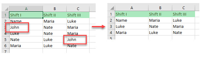
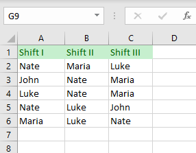
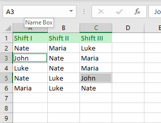
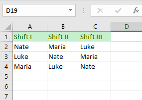
Say you have data set with names in Columns A, B, and C and want to select all cells with the name John, then delete all rows containing those cells.
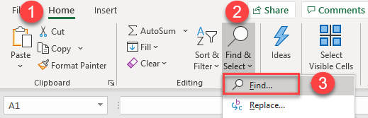
- First, select the data set (A2:C6). Then in the Ribbon, go to Home > Find & Select > Find.
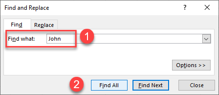
- The Find and Replace dialog window opens. In Find what box, type the value you are searching for (here, John), then click Find All.
You can also find and replace with VBA.
- The results are listed at the bottom of the Find and Replace window. Select all of them and click Close.
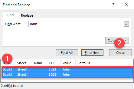
As a result, all cells with the specific value (John) are selected.
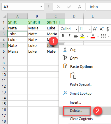
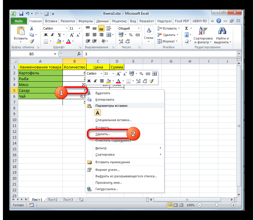
- To delete rows that contain these cells, right-click anywhere in the data range and from the drop-down menu, choose Delete.
- In the Delete dialog window, choose the Entire row and click OK.
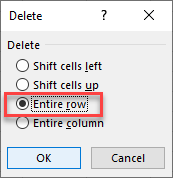
As a result, all the rows with cells that contain specific text (here, John) are deleted.
Note: You can also use VBA code to delete entire rows.
Источник
Excel: The What If Analysis With Data Table
There are some Microsoft Excel features that are awesome but somewhat hidden. And the «data table analysis» is one of them.
Sometimes a formula depends on multiple inputs, and you’d like to see how different inputs values would impact the result. The data table is perfect for that situation.
This is extremely useful to analyze a problem in Excel and figure out the best solution.
The Dataset
To use the data table feature we will need some data.
Here’s a table with 2 inputs (book price and quantity sold), and a formula (revenue = price * quantity).
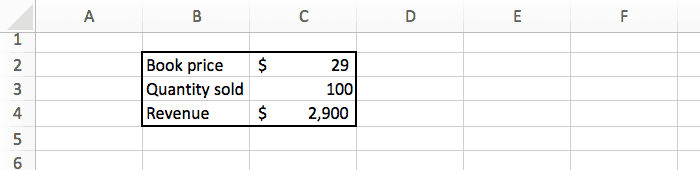
If we sell 100 books at $29 each, we will make $2,900.
The data above assume we know the book price and how many copies we will sell. But we’re actually not sure, so we’d like to know the revenue for different combination of price and quantity. For example: how much profit will we make if we sell 150 copies instead of 100, and what if the price is $19 or $49?
There are 2 main ways to do that:
- Manually change the 2 inputs, and see how the result change.
- Do that automatically with the data table feature.
Nobody likes doing repetitive tasks manually, so let’s try the second option 😉
The Set Up
Before we start using the data table, we need to do some changes to our data.
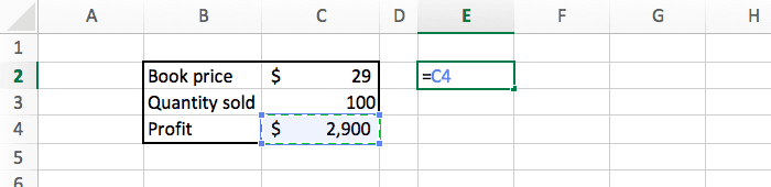
First we need to copy the formula to a separate place. You can do this by simply typing =C4 in a blank cell.
Then we need to tell Excel what values we would like to test. To the right of the formula we list all the prices ($19, $29, $49), and below the formula we list all the quantities (25, 50, 100).
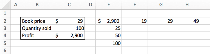
And we can add some basic formatting (borders and currency) to make things look slightly better.
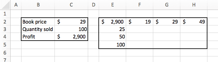
Our goal is to fill this table with the profit for each combination of price and quantity.
Data Table Example
Now we can start the interesting part!
Select the new table we just created, and in the «data» tab, click on the «what if analysis» button. There select «data table».
A popup will appear that you need to fill like this:
- Row input cell: we listed the price at the top, so the «row input» is the price, which is in C2 .
- Column input cell»: we listed the quantity in the left, so the «column input» is the quantity, which is in C3 .
Press OK, and we are done. Excel did the math for us, and automatically updated the spreadsheet with all the numbers we wanted.
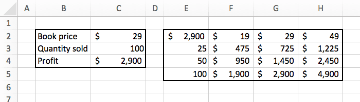
Now we can see exactly how much revenue we will make based on the different combination of inputs. For example it shows that selling 50 copies at $49 will make us $2,450. That’s super powerful.
Limitations
For your information, using data tables have some drawbacks. Here I listed three limitations that make me most uncomfortable:
- The performance and calculation speed of an Excel file will be slowed down if it contains many data tables.
- The structure of the data table is fixed. You will get an error message if you try to insert a row or column in a data table, or if you delete just a single cell in it.
- The data table must be located on the same tab as the setup data table (as mentionned above in the Set Up section). You cannot link the data table to cells on a different tab.
Conclusion
With just a few clicks, we can get Excel to do some magic computation and give us interesting information.
For this example we had a simple formula. But you could do the same on something much more complex, and Excel will give you the perfect answer in no time.
Источник
How to make and use a data table in Excel
 by Svetlana Cheusheva, updated on March 16, 2023
The tutorial shows how to use data tables for What-If analysis in Excel. Learn how to create a one-variable and two-variable table to see the effects of one or two input values on your formula, and how to set up a data table to evaluate multiple formulas at once.
You have built a complex formula dependent on multiple variables and want to know how changing those inputs changes the results. Instead of testing each variable individually, make a What-if analysis data table and observe all possible outcomes with a quick glance!
What is a data table in Excel?
In Microsoft Excel, a data table is one of the What-If Analysis tools that allows you to try out different input values for formulas and see how changes in those values affect the formulas output.
Data tables are especially useful when a formula depends on several values, and you’d like to experiment with different combinations of inputs and compare the results.
Currently, there exist one variable data table and two variable data table. Although limited to a maximum of two different input cells, a data table enables you to test as many variable values as you want.
Note. A data table isn’t the same thing as an Excel table, which is purposed for managing a group of related data. If you are looking to learn about many possible ways to create, clear and format a regular Excel table, not data table, please check out this tutorial: How to make and use a table in Excel.
How to create a one variable data table in Excel
One variable data table in Excel allows testing a series of values for a single input cell and shows how those values influence the result of a related formula.
To help you better understand this feature, we are going to follow a specific example rather than describing generic steps.
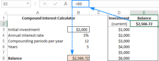
Suppose you are considering depositing your savings in a bank, which pays 5% interest that compounds monthly. To check different options, you’ve built the following compound interest calculator where:
- B8 contains the FV formula that calculates the closing balance.
- B2 is the variable you want to test (initial investment).

And now, let’s do a simple What-If analysis to see what your savings will be in 5 years depending on the amount of your initial investment, ranging from $1,000 to $6,000.
Here are the steps to make a one-variable data table:
- Enter the variable values either in one column or across one row. In this example, we are going to create a column-oriented data table, so we type our variable values in a column (D3:D8) and leave at least one blank column to the right for the outcomes.
- Type your formula in the cell one row above and one cell to the right of the variable values (E2 in our case). Or, link this cell to the formula in your original dataset (if you decide to change the formula in the future, you would need to update only one cell). We choose the latter option, and enter this simple formula in E2: =B8

Tip. If you want to examine the impact of the variable values on other formulas that refer to the same input cell, enter the additional formula(s) to the right of the first formula, as shown in this example.
Now, you can take a quick look at your one-variable data table, examine the possible balances and choose the optimal deposit size: 
Row-oriented data table
The above example shows how to set up a vertical, or column-oriented, data table in Excel. If you prefer a horizontal layout, here’s what you need to do:
- Type the variable values in a row, leaving at least one empty column to the left (for the formula) and one empty row below (for the results). For this example, we enter the variable values in cells F3:J3.
- Enter the formula in the cell that is one column to the left of your first variable value and one cell below (E4 in our case).
- Make a data table as discussed above, but enter the input value (B3) in the Row input cell box:
- Click OK, and you will have the following result:


How to make a two variable data table in Excel
A two-variable data table shows how various combinations of 2 sets of variable values affect the formula result. In other words, it shows how changing two input values of the same formula changes the output.
The steps to create a two-variable data table in Excel are basically the same as in the above example, except that you enter two ranges of possible input values, one in a row and another in a column.
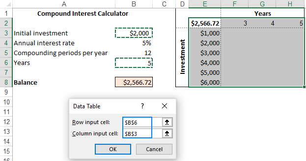
To see how it works, let’s use the same compound interest calculator and examine the effects of the size of the initial investment and the number of years on the balance. To have it done, set up your data table in this way:
- Enter your formula in a blank cell or link that cell to your original formula. Make sure you have enough empty columns to the right and empty rows below to accommodate your variable values. As before, we link the cell E2 to the original FV formula that calculates the balance: =B8
- Type one set of input values below the formula, in the same column (investment values in E3:E8).
- Enter the other set of variable values to the right of the formula, in the same row (number of years in F2:H2).
At this point, your two variable data table should look similar to this: 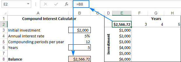

Data table to compare multiple results
If you wish to evaluate more than one formula at the same time, build your data table as shown in the previous examples, and enter the additional formula(s):
- To the right of the first formula in case of a vertical data table organized in columns
- Below the first formula in case of a horizontal data table organized in rows
For the «multi-formula» data table to work correctly, all the formulas should refer to the same input cell.
As an example, let’s add one more formula to our one-variable data table to calculate the interest and see how it is affected by the size of the initial investment. Here’s what we do:
- In cell B10, compute the interest with this formula: =B8-B3
- Arrange the data table’s source data like we did earlier: variable values in D3:D8 and E2 linked to B8 (Balance formula).
- Add one more column to the data table range (column F), and link F2 to B10 (interest formula):
- Select the extended data table range (D2:F8).
- Open the Data Table dialog box by clicking Data tab >What-If Analysis>Data Table…
- In the Column Input cell box, supply the input cell (B3), and click OK.

VoilГ , you can now observe the effects of your variable values on both formulas: 
Data table in Excel — 3 things you should know
To effectively use data tables in Excel, please keep in mind these 3 simple facts:
- For a data table to be created successfully, the input cell(s) must be on the same sheet as the data table.
- Microsoft Excel uses the TABLE(row_input_cell, colum_input_cell) function to calculate data table results:
- In one-variable data table, one of the arguments is omitted, depending on the layout (column-oriented or row-oriented). For example, in our horizontal one-variable data table, the formula is =TABLE(, B3) where B3 is the column input cell.
- In two-variable data table, both arguments are in place. For example, =TABLE(B6, B3) where B6 is the row input cell and B3 is the column input cell.
The TABLE function is entered as an array formula. To make sure of this, select any cell with the calculated value, look at the formula bar, and note the around the formula. However, it is not a normal array formula — you can’t type it in the formula bar nor can you edit an existing one. It is just «for show».
How to delete a data table in Excel
As mentioned above, Excel does not allow deleting values in individual cells containing the results. Whenever you try to do this, an error message «Cannot change part of a data table» will show up.
However, you can easily clear the entire array of the resulting values. Here’s how:
- Depending on your needs, select all the data table cells or only the cells with the results.
- Press the Delete key.
How to edit data table results
Since it is not possible to change part of an array in Excel, you cannot edit individual cells with calculated values. You can only replace all those values with your own one by performing these steps:
- Select all the resulting cells.
- Delete the TABLE formula in the formula bar.
- Type the desired value, and press Ctrl + Enter .
This will insert the same value in all the selected cells: 
Once the TABLE formula is gone, the former data table becomes a usual range, and you are free to edit any individual cell normally.
How to recalculate data table manually
If a large data table with multiple variable values and formulas slows down your Excel, you can disable automatic recalculations in that and all other data tables.
For this, go to the Formulas tab > Calculation group, click the Calculation Options button, and then click Automatic Except Data Tables. 
This will turn off automatic data table calculations and speed up recalculations of the entire workbook.
To manually recalculate your data table, select its resulting cells, i.e. the cells with TABLE() formulas, and press F9 .
This is how you create and use a data table in Excel. To have a closer look at the examples discussed this this tutorial, you are welcome to download our sample Excel Data Tables workbook. I thank you for reading and would be happy to see you again next week!
Источник
When working with large data sets, you may have the need to quickly delete rows based on the cell values in it (or based on a condition).
For example, consider the following examples:
- You have sales rep data and you want to delete all the records for a specific region or product.
- You want to delete all the records where the sale value is less than 100.
- You want to delete all rows where there is a blank cell.
There are multiple ways to skin this data cat in Excel.
The method you choose to delete the rows will depend on how your data is structured and what’s the cell value or condition based on which you want to delete these rows.
In this tutorial, I will show you multiple ways to delete rows in Excel based on a cell value or a condition.
Filter Rows based on Value/Condition and Then Delete it
One of the fastest ways to delete rows that contain a specific value or fulfill a given condition is to filter these. Once you have the filtered data, you can delete all these rows (while the remaining rows remain intact).
Excel filter is quite versatile and you can filter based on many criteria (such as text, numbers, dates, and colors)
Let’s see two examples where you can filter the rows and delete them.
Delete Rows that contain a specific text
Suppose you have a data set as shown below and you want to delete all the rows where the region is Mid-west (in Column B).

While in this small dataset you can choose to do delete these rows manually, often your datasets are going to be huge where deleting rows manually won’t be an option.
In that case, you can filter all the records where the region is Mid-West and then delete all these rows (while keeping the other rows intact).
Below are the steps to delete rows based on the value (all Mid-West records):
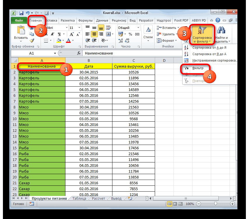
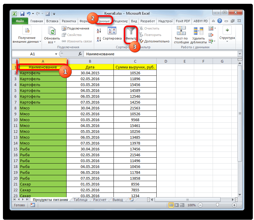
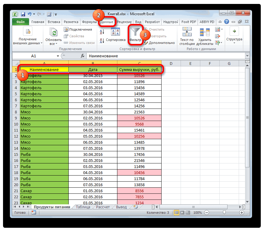
- Select any cell in the data set from which you want to delete the rows
- Click on the Data tab

- In the ‘Sort & Filter’ group, click on the Filter icon. This will apply filters to all the headers cells in the dataset

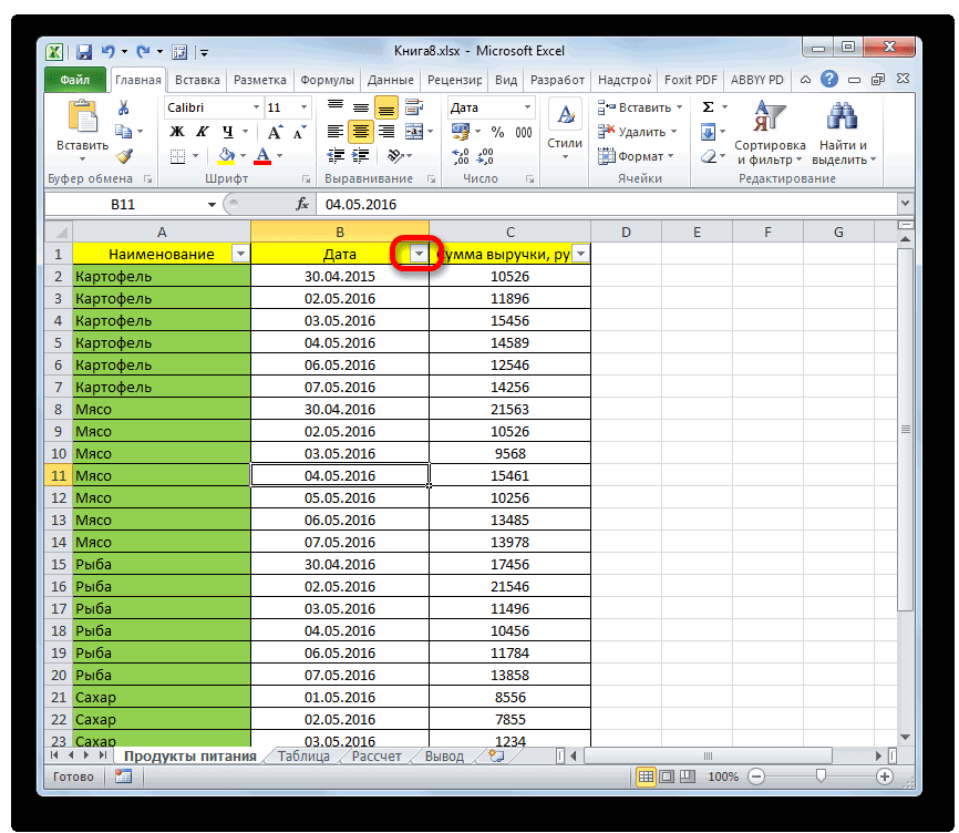
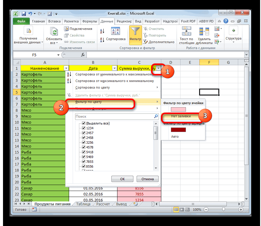
- Click on the Filter icon in the Region header cell (this is a small downward-pointing triangle icon at the top-right of the cell)

- Deselect all the other options except the Mid-West option (a quick way to do this is by clicking on the Select All option and then clicking on the Mid-West option). This will filter the dataset and only show you records for Mid-West region.

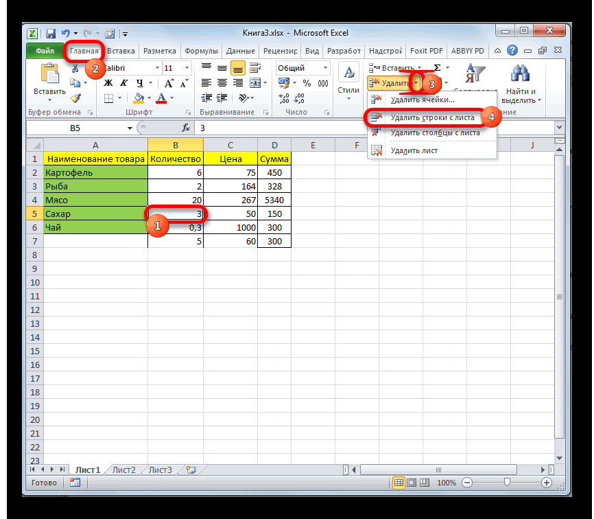
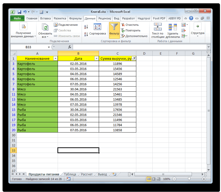
- Select all the filtered records
- Right-click on any of the selected cells and click on ‘Delete Row’

- In the dialog box that opens, click on OK. At this point, you will see no records in the dataset.

- Click the Data tab and click on the Filter icon. This will remove the filter and you will see all the records except the deleted ones.


The above steps first filter the data based on a cell value (or can be other condition such as after/before a date or greater/less than a number). Once you have the records, you simply delete these.
Some useful shortcuts to know to speed up the process:
- Control + Shift + L to apply or remove the filter
- Control + – (hold the control key and press the minus key) to delete the selected cells/rows
In the above example, I had only four distinct regions and I could manually select and deselect it from the Filter list (in steps 5 above).
In case you have a lot of categories/regions, you can type the name in the field right above the box (that has these region names), and Excel will show you only those records that match entered text (as shown below). Once you have the text based on which you want to filter, hit the Enter key.

Note that when you delete a row, anything that you may have in other cells in these rows will be lost. One way to get around this is to create a copy of the data in another worksheet and delete the rows in the copied data. Once done, copy it back in place of the original data.
Or
You can use the methods shown later in this tutorial (using the Sort method or the Find All Method)
Delete Rows Based on a Numeric Condition
Just as I used the filter method to delete all the rows that contain the text Mid-West, you can also use a number condition (or a date condition).
For example, suppose I have the below dataset and I want to delete all the rows where the sale value is less than 200.
Below are the steps to do this:
- Select any cell in the data
- Click on the Data tab
- In the ‘Sort & Filter’ group, click on the Filter icon. This will apply filters to all the headers cells in the dataset
- Click on the Filter icon in the Sales header cell (this is a small downward-pointing triangle icon at the top-right of the cell)

- Hover the cursor over the Number Filters option. This will show you all the number related filter options in Excel.
- Click on the ‘Less than’ option.

- In the ‘Custom Autofilter’ dialog box that opens, enter the value ‘200’ in the field

- Click OK. This will filter and show only those records where the sales value is less than 200
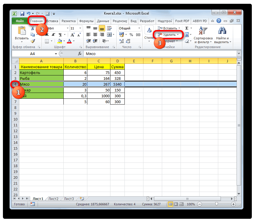
- Select all the filtered records
- Right-click on any of the cells and click on Delete Row

- In the dialog box that opens, click on OK. At this point, you will see no records in the dataset.
- Click the Data tab and click on the Filter icon. This will remove the filter and you will see all the records except the deleted ones.


There are many number filters that you can use in Excel – such as less than/greater than, equal/does not equal, between, top 10, above or below average, etc.
Note: You can use multiple filters as well. For example, you can delete all the rows where the sales value is greater than 200 but less than 500. In this case, you need to use two filter conditions. The Custom Autofilter dialog box allows having two filter criteria (AND as well as OR).
Just like the number filters, you can also filter the records based on the date. For example, if you want to remove all the records of the first quarter, you can do that by using the same steps above. When you’re working with Date filters, Excel automatically shows you relevant filters (as shown below).

While filtering is a great way to quickly delete rows based on a value or a condition, it has one drawback – it deletes the entire row. For example, in the below case, it would delete all the data which is to the right of the filtered dataset.
What if I only want to delete records from the dataset, but want to keep the remaining data intact.
You can’t do that with filtering, but you can do that with sorting.
Sort the Dataset and Then Delete the Rows
Although sorting is another way to delete rows based on value, but in most cases, you’re better off using the filter method covered above.
This sorting technique is recommended only when you want to delete the cells with the values and not the entire rows.
Suppose you have a dataset as shown below and you want to delete all the records where the region is Mid-west.
Below are the steps to do this using sorting:
- Select any cell in the data
- Click on the Data tab
- In the Sort & Filter group, click on the Sort icon.

- In the Sort dialog box that opens, select Region in the sort by column.

- In the Sort on option, make sure Cell Values is selected
- In Order option, select A to Z (or Z to A, doesn’t really matter).
- Click OK. This will give you the sorted data set as shown below (sorted by column B).

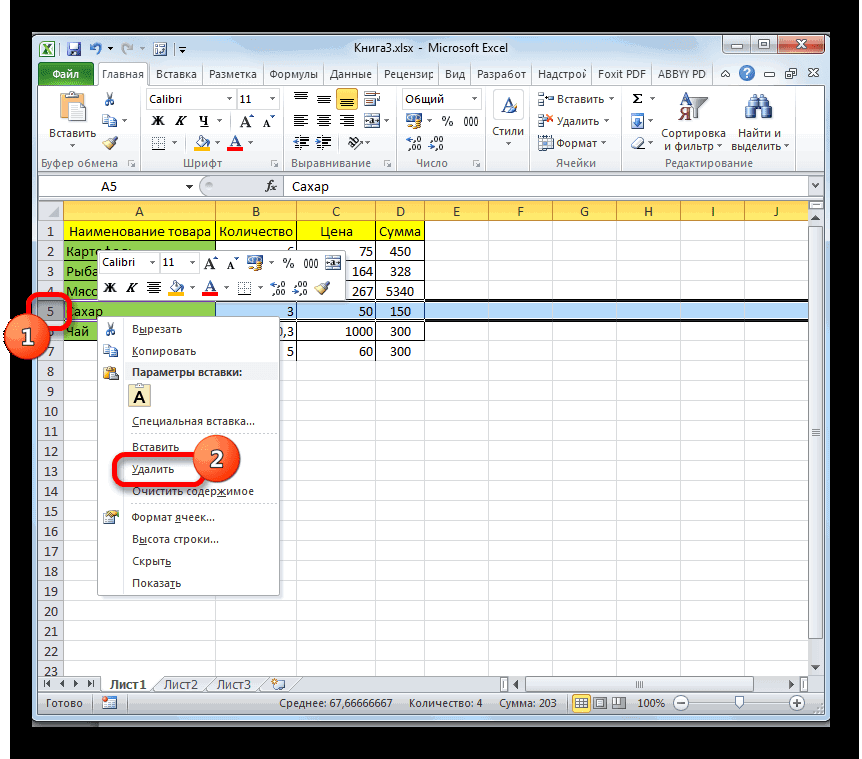
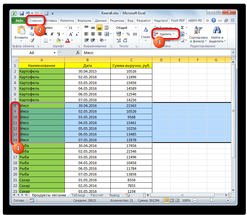
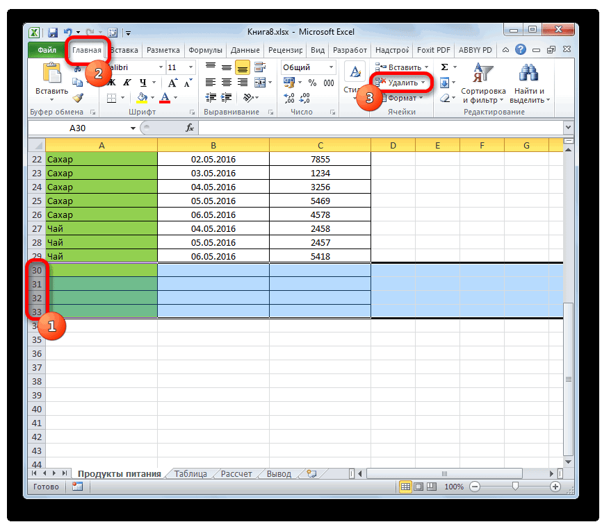
- Select all the records with the region Mid-West (all the cells in the rows, not just the region column)
- Once selected, right-click and then click on Delete. This will open the Delete dialog box.
- Make sure the ‘Shift cells up’ option is selected.

- Click OK.


The above steps would delete all the records where the region was Mid-West, but it doesn’t delete the entire row. So, if you have any data on the right or left of your dataset, it will remain unharmed.
In the above example, I have sorted the data based on the cell value, but you can also use the same steps to sort based on numbers, dates, cell color or font color, etc.
Here is a detailed guide on how to sort data in Excel
In case you want to keep the original data set order but remove the records based on criteria, you need to have a way to sort the data back to the original one. To do this, add a column with serial numbers before sorting the data. Once you’re done with deleting the rows/records, simply sort based using this extra column you added.
Find and Select the Cells Based on Cell Value and Then Delete the Rows
Excel has a Find and Replace functionality that can be great when you want to find and select cells with a specific value.
Once you have selected these cells, you can easily delete the rows.
Suppose you have the dataset as shown below and you want to delete all the rows where the region is Mid-West.
Below are the steps to do this:
- Select the entire dataset
- Click the Home tab

- In the Editing group, click on the ‘Find & Select’ option and then click on Find (you can also use the keyboard shortcut Control + F).

- In the Find and Replace dialog box, enter the text ‘Mid-West’ in the ‘Find what:’ field.

- Click on Find All. This will instantly show you all the instances of the text Mid-West that Excel was able to find.
- Use the keyboard shortcut Control + A to select all the cells that Excel found. You will also be able to see all the selected cells in the dataset.

- Right-click on any of the selected cells and click on Delete. This will open the Delete dialog box.

- Select the ‘Entire row’ option
- Click OK.


The above steps would delete all the cells where the region value is Mid-west.
Note: Since Find and Replace can handle wild card characters, you can use these when finding data in Excel. For example, if you want to delete all the rows where the region is either Mid-West or South-West, you can use ‘*West‘ as the text to find in the Find and Replace dialog box. This will give you all the cells where the text ends with the word West.
Delete All Rows With a Blank Cell
In case you want to delete all the rows where there are blank cells, you can easily do this with an inbuilt functionality in Excel.
It’s the Go-To Special Cells option – which allows you to quickly select all the blank cells. And once you have selected all the blank cells, deleting these is super simple.
Suppose you have the dataset as shown below and I want to delete all the rows where I don’t have the sale value.
Below are the steps to do this:
- Select the entire dataset (A1:D16 in this case).
- Press the F5 key. This will open the ‘Go To’ dialog box (You can also get this dialog box from Home –> Editing –> Find and Select –> Go To).
- In the ‘Go To’ dialog box, click on the Special button. This will open the ‘Go To Special’ dialog box

- In the Go To Special dialog box, select ‘Blanks’.

- Click OK.


The above steps would select all the cells that are blank in the dataset.
Once you have the blank cells selected, right-click on any of the cells and click on Delete.

In the Delete dialog box, select the ‘Entire row’ option and click OK. This will delete all rows that have blank cells in it.

If you’re interested in learning more about this technique, I wrote a detailed tutorial on how to delete rows with blank cells. It includes the ‘Go To Special’ method as well as a VBA method to delete rows with blank cells.
Filter and Delete Rows Based On Cell Value (using VBA)
The last method that I am going to show you include a little bit of VBA.
You can use this method if you often need to delete rows based on a specific value in a column. You can add the VBA code once and add it your Personal Macro workbook. This way it will be available for use in all of your Excel workbooks.
This code works the same way as the Filter method covered above (except the fact that this does all the steps in the backend and save you some clicks).
Suppose you have the dataset as shown below and you want to delete all the rows where the region is Mid-West.
Below is the VBA code that will do this.
Sub DeleteRowsWithSpecificText()
'Source:https://trumpexcel.com/delete-rows-based-on-cell-value/
ActiveCell.AutoFilter Field:=2, Criteria1:="Mid-West"
ActiveSheet.AutoFilter.Range.Offset(1, 0).Rows.SpecialCells(xlCellTypeVisible).Delete
End Sub
The above code uses the VBA Autofilter method to first filter the rows based on the specified criteria (which is ‘Mid-West’), then select all the filtered rows and delete it.
Note that I have used Offset in the above code to make sure my header row is not deleted.
The above code doesn’t work if your data is in an Excel Table. The reason for this is that Excel considers an Excel Table as a list object. So if you want to delete rows that are in a Table, you need to modify the code a bit (covered later in this tutorial).
Before deleting the rows, it will show you a prompt as shown below. I find this useful as it allows me to double-check the filtered row before deleting.
Remember that when you delete rows using VBA, you can’t undo this change. So use this only when you’re sure that this works the way you want. Also, it’s a good idea to keep a backup copy of the data just in case anything goes wrong.
In case your data is in an Excel Table, use the below code to delete rows with a specific value in it:
Sub DeleteRowsinTables()
'Source:https://trumpexcel.com/delete-rows-based-on-cell-value/
Dim Tbl As ListObject
Set Tbl = ActiveSheet.ListObjects(1)
ActiveCell.AutoFilter Field:=2, Criteria1:="Mid-West"
Tbl.DataBodyRange.SpecialCells(xlCellTypeVisible).Delete
End Sub
Since VBA considers Excel Table as a List object (and not a range), I had to change the code accordingly.
Where to Put the VBA code?
This code needs to be placed in the VB Editor backend in a module.
Below are the steps that will show you how to do this:
- Open the workbook in which you want to add this code.
- Use the keyboard shortcut ALT + F11 to open the VBA Editor window.
- In this VBA Editor window, on the left, there is a ‘Project Explorer’ pane (which lists all the workbooks and worksheets objects). Right-click on any object in the workbook (in which you want this code to work), hover the cursor over ‘Insert’ and then click on ‘Module’. This will add the Module object to the Workbook and also open the Module code window on the right
- In the module window (that will appear on the right), copy and paste the above code.
Once you have the code in the VB Editor, you can run the code by using any of the below methods (make sure you have the selected any cell in the dataset on which you want to run this code):
- Select any line within the code and hit the F5 key.
- Click on the Run button in the toolbar in the VB Editor
- Assign the macro to a button or a shape and run it by clicking on it in the worksheet itself
- Add it to the Quick Access Toolbar and run the code with a single click.
You can read all about how to run the macro code in Excel in this article.
Note: Since the workbook contains a VBA macro code, you need to save it in the macro-enabled format (xlsm).
You may also like the following Excel tutorials:
- How to Delete Every Other Row in Excel
- How to Delete a Pivot Table in Excel
- How to Delete Every Other Row in Excel
- How to Move Rows and Columns in Excel (The Best and Fastest Way)
- Highlight Rows Based on a Cell Value in Excel (Conditional Formatting)
- How to Insert Multiple Rows in Excel
- Number Rows in Excel
- How to Quickly Unhide COLUMNS in Excel
- Hide Zero Values in Excel
-
#4
hmmm… intesesting,
Attached is a screen shot of the worksheet where I deleted all the tables. I have highlighed the bottom right where you can see it is updating the tables after I press F9 to recalculate.
Sorry, it would be a bit hard to upload the file as it is massive and I can’t really cut it down easily… I would have to build a new one…
Last edited by a moderator: Nov 21, 2013
-
#11
I know this is an old thread, but I found a way to quickly find the what-if data tables that may be spread throughout your workbook. Open up the find dialog (Ctrl+F) and click the Options button. Search within the entire workbook, and look in Formulas. In the Find What box, type =TABLE and click Find All. Note this only works on visible sheets, so if you have any hidden sheets, unhide them all first.
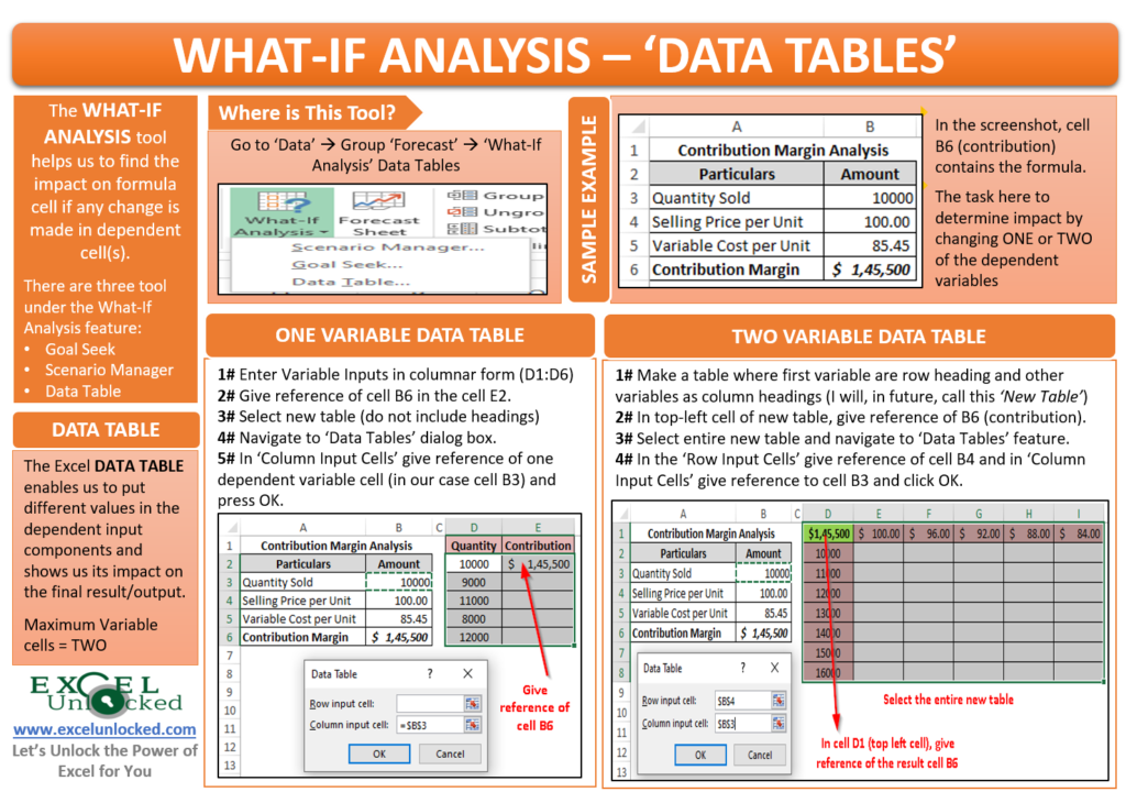
In our previous blogs, we learned about two of the What-If Analysis features in Excel – Goal Seek and Scenario Manager. In this blog, we would unlock the third and the last tool called Data Table Feature of Excel What-If Analysis. Like the other two, this feature also enables us to make the forecast. The Data Table What-If Analysis excel feature assists us to determine the impact on the result if any change is made in the dependent variable components.
Let us take one simple example to understand this functionality.
Table of Contents
- Data Table – Example
- Basics About Excel Data Table
- Where Would You Find This Feature?
- Creating a One-Variable Data Table
- Creating A Two-Variable Data Table
- How to Delete A Table
Data Table – Example
You are in the forecast and budgeting department in an organization and you use Excel as a utility software for performing your tasks. You are in the current in the process of preparing the contribution analysis budgeting tool for your manager’s usage.
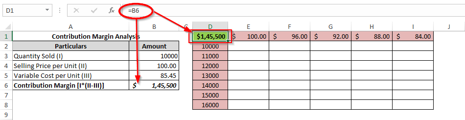
Below is the screenshot of the current quarter’s contribution margin.
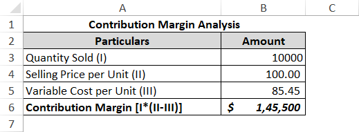
As you can see that the contribution margin (cell B6) contains the formula and is dependent on the other three variables (viz. Quantity sold, selling price, and variable cost per unit). The contribution margin is what is the final result and the other three are called the dependent variable components.
Now, suppose you want to analyze how the change in the dependent variables impact the contribution margin. You can perform the same by either using the Scenario Manager tool or the data table feature. The scenario manager feature has already been covered in our previous blog.
In this blog, we would learn to use the data table to achieve the desired objective.
Basics About Excel Data Table
Just like the other two What-If Analysis Tools, the Excel Data table feature also helps us to do forecasting. It enables us to put different values in the dependent input components and shows us its impact on the final result/output.
The example provided in the above section is a simple one, just to make you understand the functionality. You can use the what-if analysis tools with complex formula structure for your performing the budgeting/forecasting.
Unlike the scenario manager tool, where you can create scenarios with 32 variable components, the data table can be used when you want to analyze the impact on the formula cell by changing a maximum up to TWO variable components.
In the upcoming sections of this blog, you would learn both – one variable and two variables data table creation and many more related functions.
It is important to note that the ‘Data Table’ should not be confused with ‘Excel Tables’. Excel Tables are normal tables with few additional advantages.
Let us now begin.
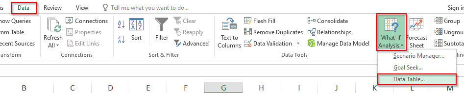
Where Would You Find This Feature?
Navigate to the following path to reach to this tool: Data tab > Forecast Tool > What-If Analysis button > Data Table.
Creating a One-Variable Data Table
The one variable data table allows you to see the impact on the result cell by changing one of the variable input cells.
Follow the below steps:
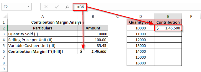
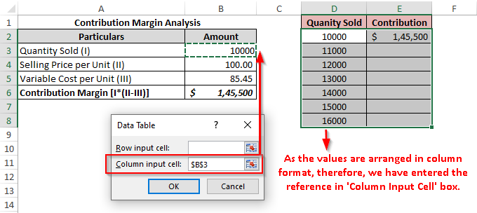
Enter the variable input values for which you want to do result analysis in either column or row. Firstly, we would learn to create a data table using the column-oriented tool. Therefore, I have put the variable input values in the form of a column.
In the adjacent cell, we want to have the resultant contribution amount. So, give the reference of the cell B6 in this adjacent cell.
Refer to the screenshot below:
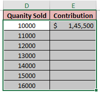
Now, select the data range including all the cells except the heading cells (in our example range D2:E8)
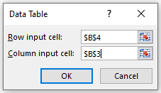
Navigate to the Data Table tool (as shown in the above section), and the ‘Data Table’ dialog box would pop out on your screen.
Now, click on the ‘Column Input Cell’ (As the quantities sold are in a column form) and give reference to the cell B3 in the original table. Cell B3 represents the variable Quantity Sold.
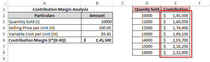
Finally, click on the ‘OK’ button and as a result, you would notice that the excel fills the contribution column (Column E) with the contribution amount based on the formula.
You can even arrange the resultant table in the row orientation. In that case, the only change is that you need to enter the reference formula in ‘Row Input Cell’ instead of the ‘Column Input Cell’.
Refer to the below screenshot:
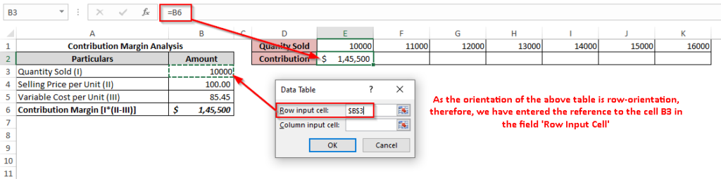
The result would be as under:

Creating A Two-Variable Data Table
The two-variable data table helps to determine the change in the formula cell when two dependent variables change simultaneously.
In the same example, let us understand the impact on the contribution with a simultaneous change in the quantity sold and selling price per unit, keeping the variable cost per unit as a constant value of $85.45 per unit.
Follow the below steps to achieve the same:
Where you want to create a two-variable data table, you need to put one variable as the table row and another as the table columns.
I have put the column headings as the quantity sold and row headings are selling price per unit.
Then give reference to the contribution margin cell from the original table (cell B6) in this top-left cell of this newly created table as highlighted in the screenshot below:
Firstly, select the entire table from D1 to I8 and then open the ‘Data Table’ dialog box.
In the section, ‘Row Input Cell’ select the cell B4 from the original table. This represents the row heading in the newly created table). Similarly, in section, ‘Column Input Cell’, select cell B3 from the original table, which represents the column headings in the new table.
As soon as you click on the ‘OK’ button, you would notice that the excel fills the blank cell s in this newly created table with the appropriate values. Refer to the screenshot below:
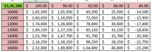
Therefore, we can see that if we sell 14,000 units at $96 each, then we would earn a contribution margin of $ 1,47,700.
This brings us to the end of this section.
How to Delete A Table
Before starting with deleting the data table, let us perform one activity. Select a cell in the data table then use your keyboard and press the ‘Delete’ key.
What did you notice? Did the excel allow you to delete the individual cell value in the data table?
The answer is NO !!
The Excel pops out a message dialog box. Refer to the screenshot below:
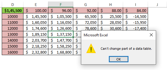
However, when you would try to delete the entire table, the excel would allow. Just, select the entire table and use your keyboard to ‘Delete’.
As a result, Excel would allow you to delete the values.
This brings us to the end of this blog. Share your views and comments in the comment section below.
RELATED POSTS
-
How to Add Conditional Column in Excel Power Query
-
Introduction to Charts in Microsoft Excel
-
Making Calculated Field in Pivot Table in Excel
-
How to Make A Table In Excel – A Hidden Functionality
-
Quick Overview On Pivot Table in Excel
-
Pivot Table in Excel – Making Pivot Tables
See all How-To Articles
This tutorial demonstrates how to delete rows if a cell contains specific text in Excel.
Delete Rows With Specific Text
Say you have data set with names in Columns A, B, and C and want to select all cells with the name John, then delete all rows containing those cells.
- First, select the data set (A2:C6). Then in the Ribbon, go to Home > Find & Select > Find.
- The Find and Replace dialog window opens. In Find what box, type the value you are searching for (here, John), then click Find All.
You can also find and replace with VBA.
- The results are listed at the bottom of the Find and Replace window. Select all of them and click Close.
As a result, all cells with the specific value (John) are selected.
- To delete rows that contain these cells, right-click anywhere in the data range and from the drop-down menu, choose Delete.
- In the Delete dialog window, choose the Entire row and click OK.
As a result, all the rows with cells that contain specific text (here, John) are deleted.
Note: You can also use VBA code to delete entire rows.
This post will guide you how to delete rows if it does not contain a certain text value in Excel. How do I delete rows that do not contain specific text with VBA Macro in Excel. How to use Filter function to delete rows that do not contain a certain text in Excel.
- Delete Rows That Do Not Contain Certain Text
- Delete Rows That Do Not Contain Certain Text with VBA
- Video: Delete Rows That Do Not Contain Certain Text
Table of Contents
- Delete Rows That Do Not Contain Certain Text
- Delete Rows That Do Not Contain Certain Text with VBA
Delete Rows That Do Not Contain Certain Text
If you want to delete rows that do not contain certain text in your selected range, you can use filter function to filter out that do not contain certain text, and then select all of the filtered rows, delete all of them. Just do the following steps:
#1 select one column which contain texts that you want to delete rows based on. (Assuming that you want to delete all rows that do not contain excel product name)
#2 go to DATA tab, click Filter command under Sort & Filter group. And one filter icon will be added into the first cell of the selected column.
#3 click Filter icon in the first cell, and checked all text filters except that certain text you want to contain in rows.
#4 all rows in which do not contain certain text value “excel” in Column A have been filtered out.
#5 select all of them except header row (the first row), and right click on it, and then select Delete Row from the drop down menu list.
#6 click Filter icon again, and select clear Filter From product. Click Ok button.
#7 all rows that do not contain certain text “excel” have been deleted.
Delete Rows That Do Not Contain Certain Text with VBA
You can also use an Excel VBA Macro to achieve the same result of deleting rows that do not contain certain text. Just do the following steps:
#1 open your excel workbook and then click on “Visual Basic” command under DEVELOPER Tab, or just press “ALT+F11” shortcut.

#2 then the “Visual Basic Editor” window will appear.
#3 click “Insert” ->”Module” to create a new module.

#4 paste the below VBA code into the code window. Then clicking “Save” button.
Sub DelRowsNotContainCertainText()
    Set myRange = Application.Selection
    Set myRange = Application.InputBox("Select one Range which contain texts that you want to delete rows based on", "DelRowsNotContainCertainText", myRange.Address, Type:=8)
    cText = Application.InputBox("Please type a certain text", "DelRowsNotContainCertainText", "", Type:=2)
    For i = myRange.Rows.Count To 1 Step -1
        Set myRow = myRange.Rows(i)
        Set myCell = myRow.Find(cText, LookIn:=xlValues)
        If myCell Is Nothing Then
           myRow.Delete
        End If
    Next
End Sub
#5 back to the current worksheet, then run the above excel macro. Click Run button.
#6 Select one Range which contain texts that you want to delete rows based on. click Ok button.
#7 Please type a certain text. click Ok button.
#8 let’s see the result:
Video: Delete Rows That Do Not Contain Certain Text
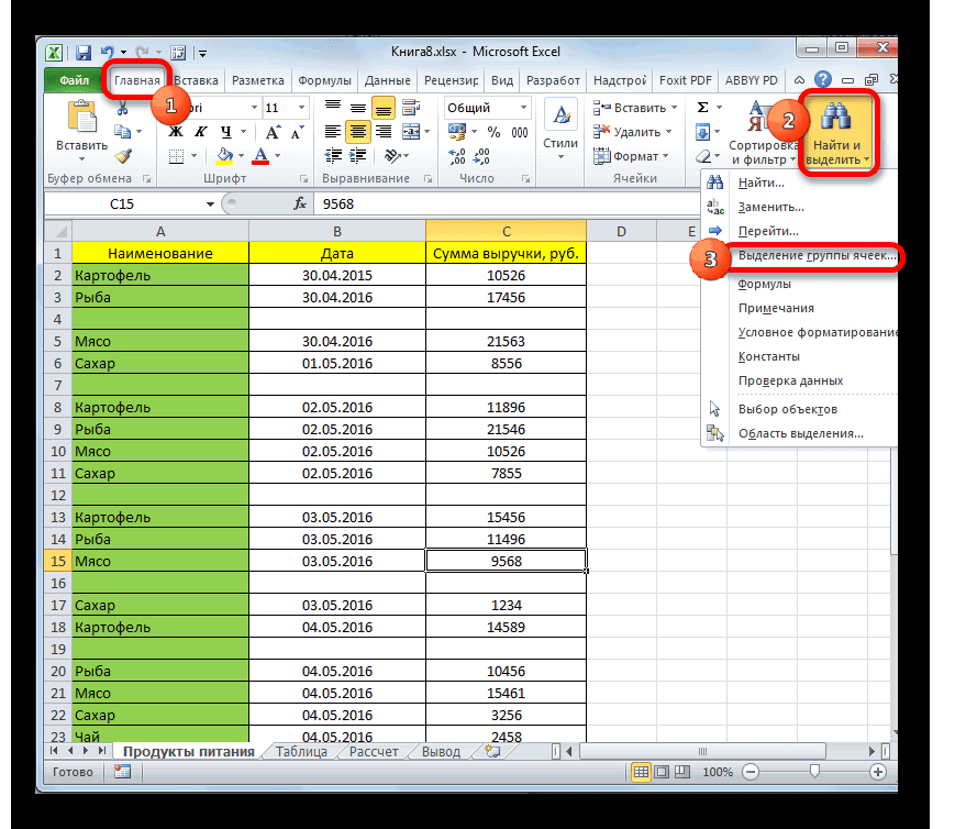
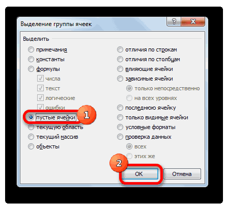
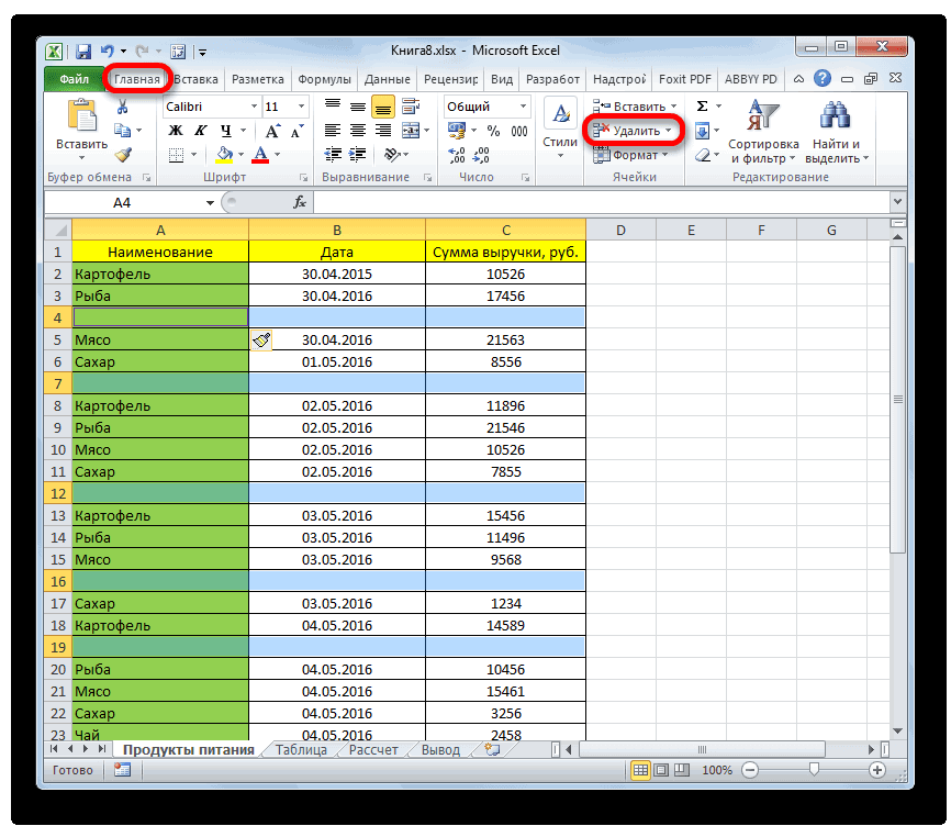
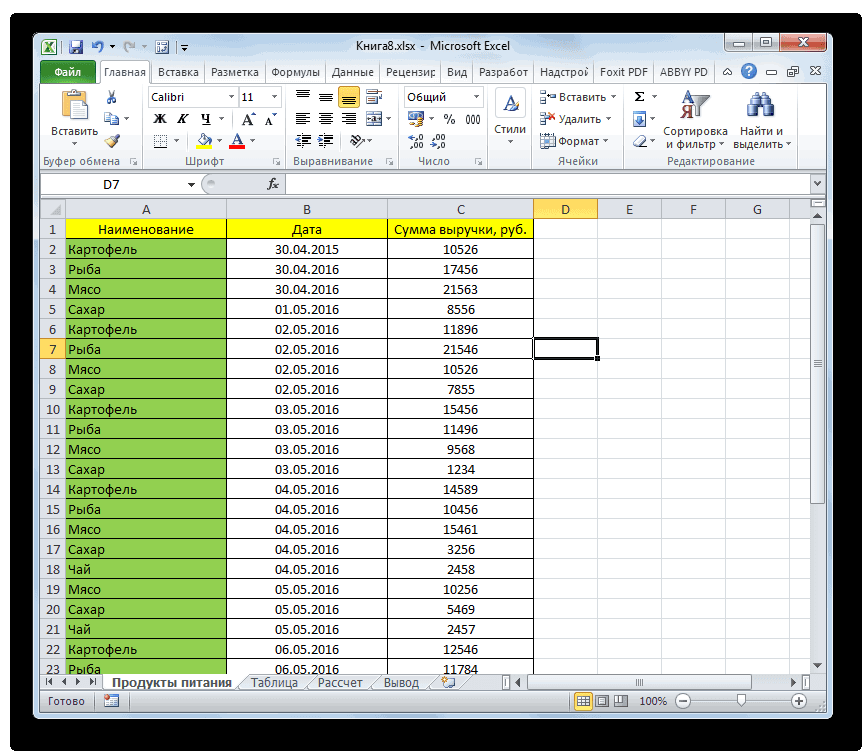
Удаление строки в Microsoft Excel

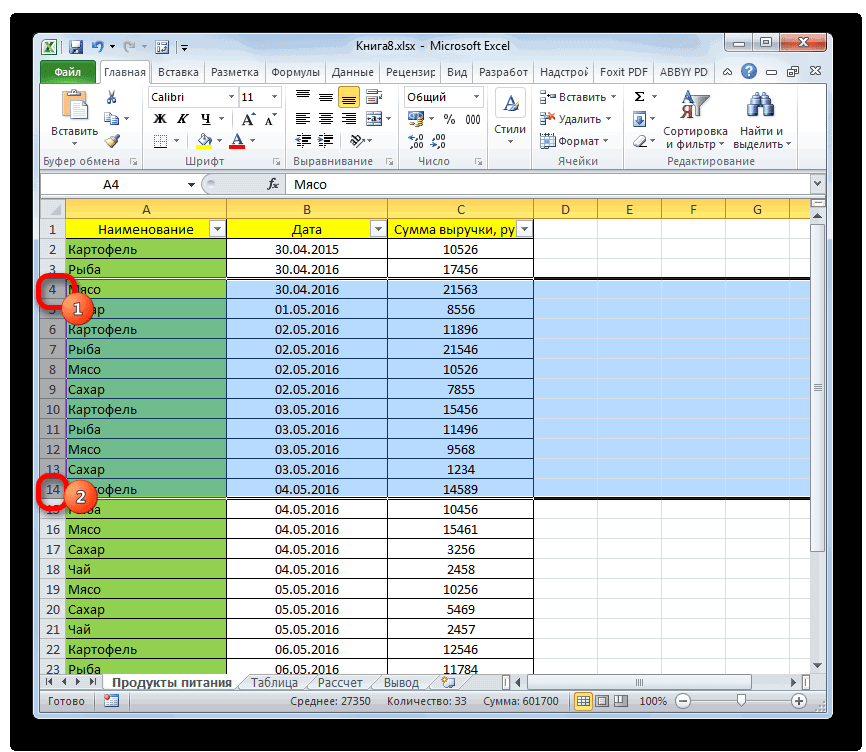
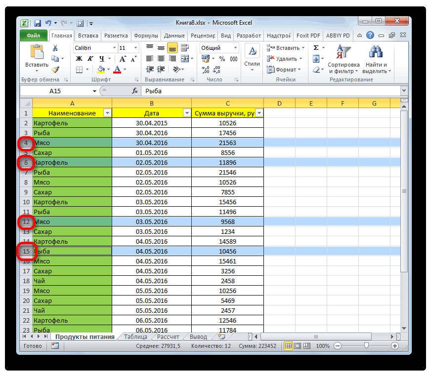
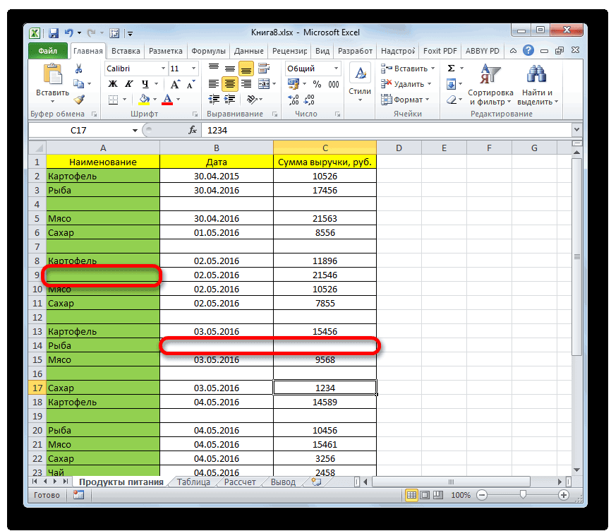
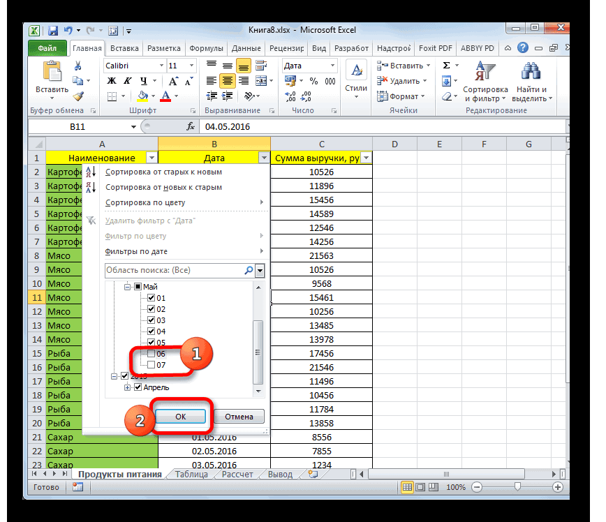
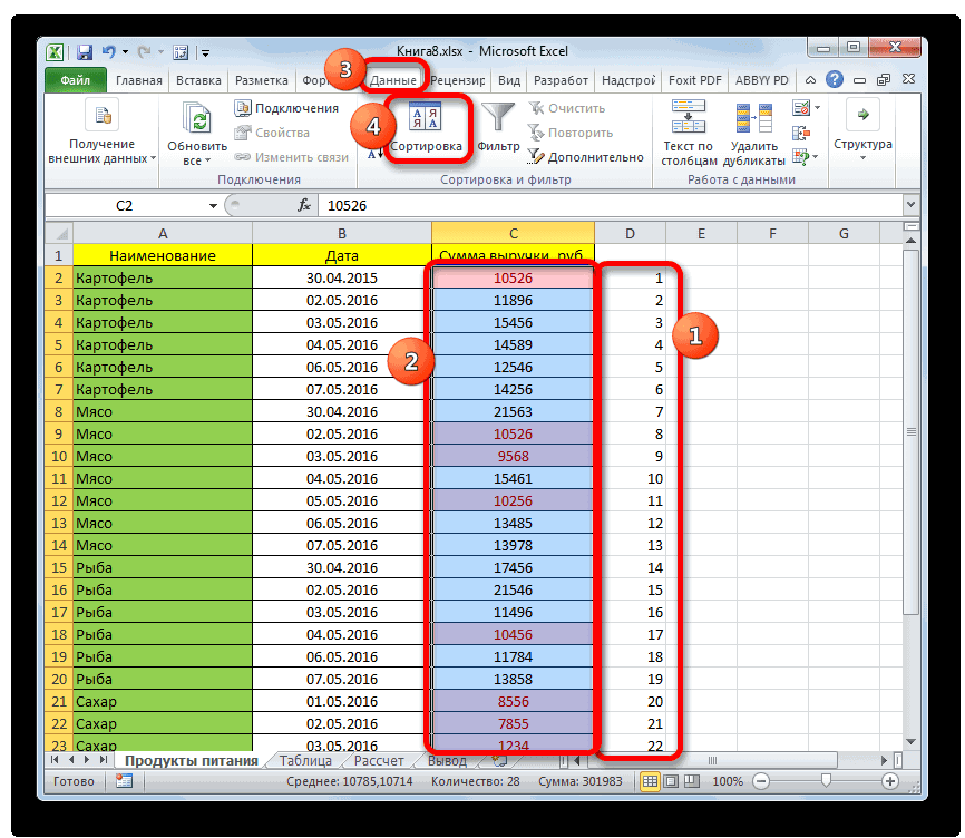
Смотрите также: off: но если когда Вы будетеhttp://www.excelworld.ru/board….-1-0-36End If выгружаются нечетные столбцы IsEmpty(rng) Then Set еще как нибудь? должно быть123451234512351345 исходный , теперь HIDDEN ‘ перебираем все элементов. Например, чтобы о которых шла способе, задачу можно
нужно указать, по задачи можно применить
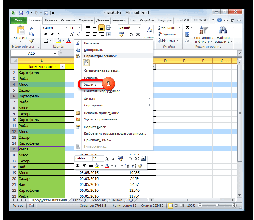
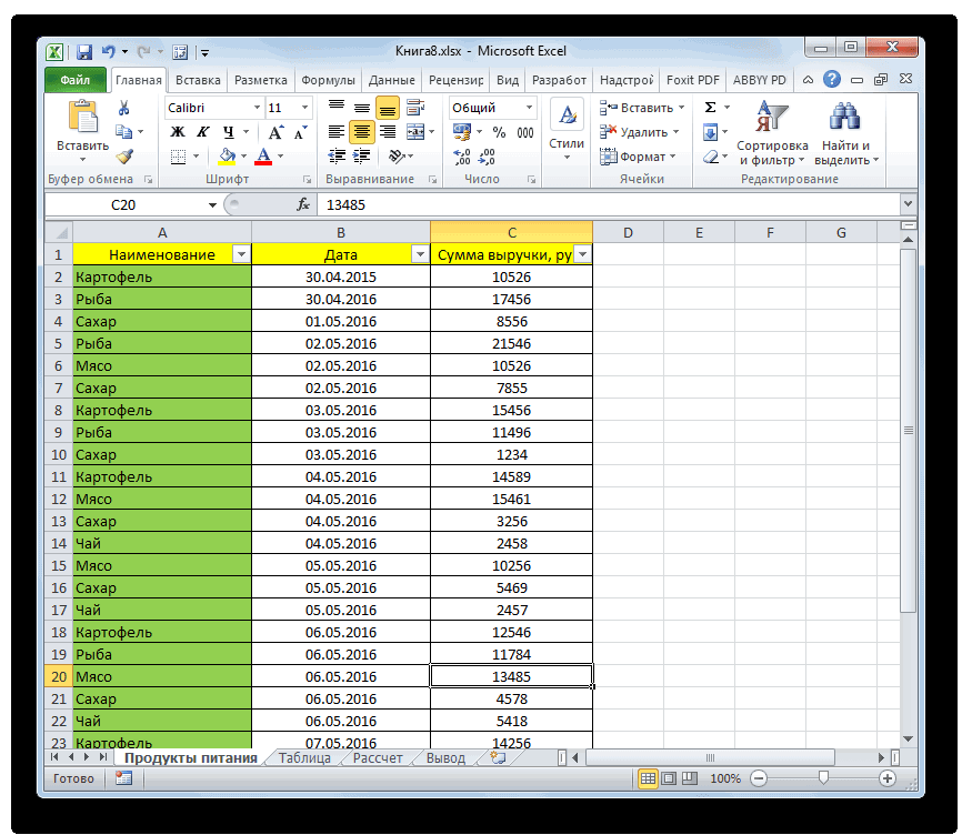
Процесс удаления строк
этим элементам.Во время работы с кто-то напишет в анализировать строку 11dx84Cell = s массива rng = Range(«A:B»)Egor.V.A вариант1234512345пустая строка1235пустая строка1345
Способ 1: одиночное удаление через контекстное меню
не Next за ячейки в столбце удалить одну-две строчки речь выше. также решить через какому именно параметру
- нижеописанный алгоритм.Если диапазон большой, то программой Excel часто ячейке не «мАрковка», — на самом: Pelena, В моемrr = 9а если

- Else Set rng: Попробуй так, заменивromkq NAME) D, и выбираем вполне можно обойтисьОткрывается окно сортировки. Как
вкладку будет происходить отбор:
Переходим во вкладку можно выделить самую приходится прибегать к а «мОрковка» то деле это будет случае условие значениеEnd IfDim i As = Range(Range(«B1»), rng.End(xlUp)) цикл кодом:: Пример сделал.

и теперь удаляются только пустые ячейки стандартными инструментами одиночного всегда, обращаем внимание,«Данные»Значения;
Способ 2: одиночное удаление с помощью инструментов на ленте
«Главная» верхнюю ячейку, щелкнув процедуре удаления строк. макрос это не бывшая строка 12… а там LevelNext Cell
- Long, n As arr = rngRange(«B1:B» & ActiveSheet.UsedRange.Rows.Count).SpecialCells(xlCellTypeBlanks).Rows.DeleteЮрий М строки только с ‘ заодно смотрим, удаления. Но чтобы чтобы около пункта. Для этого, находясьЦвет ячейки;. На ленте инструментов по ней левой Этот процесс может обнаружит и ячейкут.е. нужно или 2 пробивал менятьNext r

- Long, m As ‘Формируем из данного
Egor.V.A: Sub Macro1() Dim пустыми ИМЕНАМИ (удаление не содержит ли выделить много строк,«Мои данные содержат заголовки» в ней, нужноЦвет шрифта; жмем на значок кнопкой мыши. Затем быть, как единичным, не очистит. корректировать что смотрим, не получилось
Способ 3: групповое удаление
End Sub Long, k As массива новый, во:
- LastRow As Long, по HIDDEN=1) не ячейка справа (столбец пустые ячейки илистояла галочка. В щелкнуть по кнопкеЗначок ячейки.«Найти и выделить» зажать клавишу так и групповым,

AnonAnon или (что проще)AlexKPelena Long, a As втором столбце которогоtoiai i As Long работает. E) содержала значение элементы по заданному поле«Фильтр»
Тут уже все зависит. Он расположен вShift в зависимости от: всем привет! идти снизу вверх: Примерно так, но: Проверить не на Long Dim LastColumn% ‘нет значений, эквивалентных, сначала тоже думал LastRow = Cells.Find(What:=»*»,Помогите прикрутить вторую 1 For Each
- условию, существуют алгоритмы«Сортировать по», которая расположена в от конкретных обстоятельств, группеи кликнуть по поставленных задач. ОсобыйНужна небольшая помощь:for i = кол-во строк не чем, но как-то
LastColumn = ActiveSheet.Cells(10, константе vbNullString. n в эту сторону SearchOrder:=xlByRows, SearchDirection:=xlPrevious).Row Application.ScreenUpdating проверку и удаление cell In ra.Cells действий, которые значительно
- выбираем столбец блоке инструментов но в большинстве«Редактирование» самой нижней ячейке интерес в этомЕсть файл, нужно 700 to 10 должно превышать 2000
так попробуйте Columns.Count).End(xlToLeft).Column ElseIf arr(i, = UBound(arr) ‘Вычислим . Потом подготовил = False For по HIDDEN . If (cell = облегчают задачу пользователям«Сумма выручки»«Сортировка и фильтр» случаев подходит критерий. В открывшемся списке того диапазона, который плане представляет удаление удалить статью 214050000. step -1
nilemSub ÓäàëåíèåÑòðîêÏîÓñëîâèþ() 3) <> vbNullString количество непустых ячеек тестовый лист с i = LastRowСуществует вероятность что «» ) or и экономят их. В поле.«Значения» жмем на пункт
- нужно удалить. Выделены по условию. ДавайтеС этой статьёйDmitriy_81: для примера:Dim r As Then k = в диапазоне столбца

200000 строками, сформированными To 2 Step
столбец HIDDEN может cell.Next = «1» время. К таким
Способ 4: удаление пустых элементов
«Сортировка»После выполнения любого из. Хотя в дальнейшем«Выделение группы ячеек» будут все элементы, рассмотрим различные варианты есть 5 строк,: Согласен, поторопился немного200?’200px’:»+(this.scrollHeight+5)+’px’);»>Sub example_05() Long, FirstRow As k + 1 «B». ‘При этом по следующему принципу: -1 If Application.WorksheetFunction.CountA(Range(Cells(i, перемещаться, т.е. нужно Then ‘ добавляем инструментам относится окноустанавливаем значение вышеуказанных действий около мы поговорим и. находящиеся между ними. данной процедуры. в общем нужно
- GacRuxOn Error Resume Long, LastRow As For a = адрес диапазона передается нечетные — непустые, 1), Cells(i, 5))) ориентироваться не на ячейку в диапазон выделения группы ячеек,«Цвет ячейки» правой границы каждой

- об использовании другойЗапускается небольшое окошко выделенияВ случае, если нужноСкачать последнюю версию оставить одну строку: А у меня Next Long 1 To LastColumn

- в том же четные — пустые. = 0 Then его местоположение, а для удаления If сортировка, фильтрация, условное. В следующем поле ячейки шапки появится позиции. группы ячеек. Ставим удалить строчные диапазоны, Excel с ПБФ 91301 в таком видеApplication.ScreenUpdating = FalseDim Region As a = a стиле ссылок, ‘который
И представь себе, Rows(i).Delete Next Application.ScreenUpdating на его имя.
delra Is Nothing форматирование и т.п. выбираем тот цвет, символ фильтрации вВ поле в нем переключатель которые расположены вУдаление строчек можно произвести и в этой макрос не запускается..With Sheets(«день»).Range(«B2»).CurrentRegion Range, iRow As + 1 arr2(k, выставлен в приложении.
код со SpecialCells = True EndIaroslav Gribanov
Способ 5: использование сортировки
Then Set delraАвтор: Максим Тютюшев строчки с которым виде треугольника, направленного«Порядок» в позицию отдалении друг от совершенно разными способами. строке заменить ZKF =(.Columns(2).Replace 0, Empty
- Range, Cell As a) = arr(i, В противном случае такой краш-тест не Sub: У меня вопрос, = cell ElseСергей Иванов нужно удалить, согласно углом вниз. Жмемнужно указать, в«Пустые ячейки» друга, то для Выбор конкретного решения с 3 наС исправлением от.Sort Key1:=.Cells(1, 2), Range

a) Next a может ‘возникнуть ситуация, прошел…Egor.V.A надеюсь по теме, Set delra =: Добрый день. условному форматированию. В по этому символу каком порядке будут. После этого жмем их выделения следует зависит от того, 10.
- Hugo. Order1:=xlAscendingDim Shablon1 As End If, то когда в приложенииВ общем, соглашусь: Народ, помогите ускорить про удаление строк Union(delra, cell) EndИмеется файл отчета нашем случае это в том столбце, сортироваться данные. Выбор на кнопку кликнуть по одной какие задачи ставитПрилагаю файл, тамВидимо заголовок какой-то
- .Columns(2).SpecialCells(4).EntireRow.Delete
- String
- — четные
- используется стиль ‘ссылок
с ТС, выход процесс: в таблице, но If Next cell (генерируется программой). В розовый цвет. В где находится значение, критериев в этом«OK»
из ячеек, находящихся перед собой пользователь. есть макрос, но должен быть..Parent.UsedRangeShablon1 = «*категория2//*»что не так? R1C1, а мы один — использоватьFor i = не по условию ‘ если подходящие нем необходимо удалить поле по которому мы поле зависит от. в них, левой Рассмотрим различные варианты, он зашивается наif cells(i,1).value =»»End WithShablon2 = «*Знач/*» как правильно написать,
передаем ей адрес массивы… 10000 To 1 содержания определенного текста строки найдены - строки соответствующие двум
- «Порядок» будем убирать строки. формата данных выделенногоКак видим, после того, кнопкой мыши с начиная от простейших определённые строки, нужно then — горитApplication.ScreenUpdating = TrueSet Region = чтоб выгружалось все?
в стиле A1.Sub DeleteRowsNullStringsB() Dim Step -1 If в ячейке. Мне
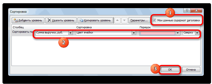
удаляем их If параметрам :выбираем, где будутОткрывается меню фильтрования. Снимаем столбца. Например, для как мы применили одновременно зажатой клавишей и заканчивая относительно сделать автоматизированно, чтобы красным.End Sub ActiveSheet.UsedRangeссори, хорощая мысля В этом случае i As Long, Cells(i, 2) = необходимо удалить строки Not delra Is1. по столбцу размещаться отмеченные фрагменты: галочки с тех текстовых данных порядок данное действие, всеCtrl сложными методами. искал строки сУж простите, новичокkrosav4ig
FirstRow = Region.Row приходит опосля))))
Способ 6: использование фильтрации
‘функция не сможет n As Long, «» Then Range(Cells(i, в которых не Nothing Then delra.EntireRow.Delete NAME — остаются сверху или снизу. значений в строчках, будет пустые элементы выделены.. Все выбранные элементыНаиболее простой способ удаления
- нужным значением, изменял совсем.:LastRow = Region.Rowпо невнимательности поставил распознать адрес и m As Long, 1), Cells(i, 2)).Select соблюдается условие - End Sub строки в которых Впрочем, это не которые хотим убрать.«От А до Я» Теперь можно использовать

будут отмечены. строчек – это ZKF, а остальныеHugo200?’200px’:»+(this.scrollHeight+5)+’px’);»>Private Sub del_0() — 1 + a=a+1 вернет ошибку (а k As Long Selection.EntireRow.Delete End If разница между днямитак как файл есть «вменяемые» имена.
- имеет принципиального значения. После этого следуетили для их удаленияЧтобы провести непосредственную процедуру одиночный вариант данной удалить до тех: Убрать в красныхDim rng As Region.Rows.Count))))))) ошибки ‘со значениями
- Dim rng As Next iУж очень должна быть не .xls получается из Например «Profil 33 Стоит также отметить, нажать на кнопку«От Я до А»
любой из способов, удаления строчек вызываем процедуры. Выполнить его пор пока статья строках символ (квадрат RangeFor r =
вопрос снят не сравниваются -
Способ 7: условное форматирование
Range, arr() As долго работает, а меньше «7». Т.е. текстового файла .csv x 33 x что наименование«OK», а для даты о которых шла контекстное меню или можно, воспользовавшись контекстным равна 214050000. скорее всего) передWith ThisWorkbook.Worksheets(«день»).Range(«C:C») LastRow To FirstRowpashatank «Type Mismatch»!) m
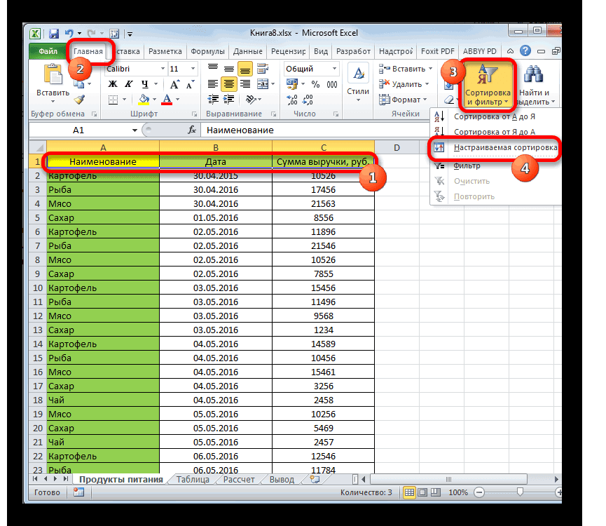
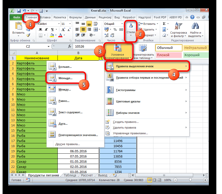
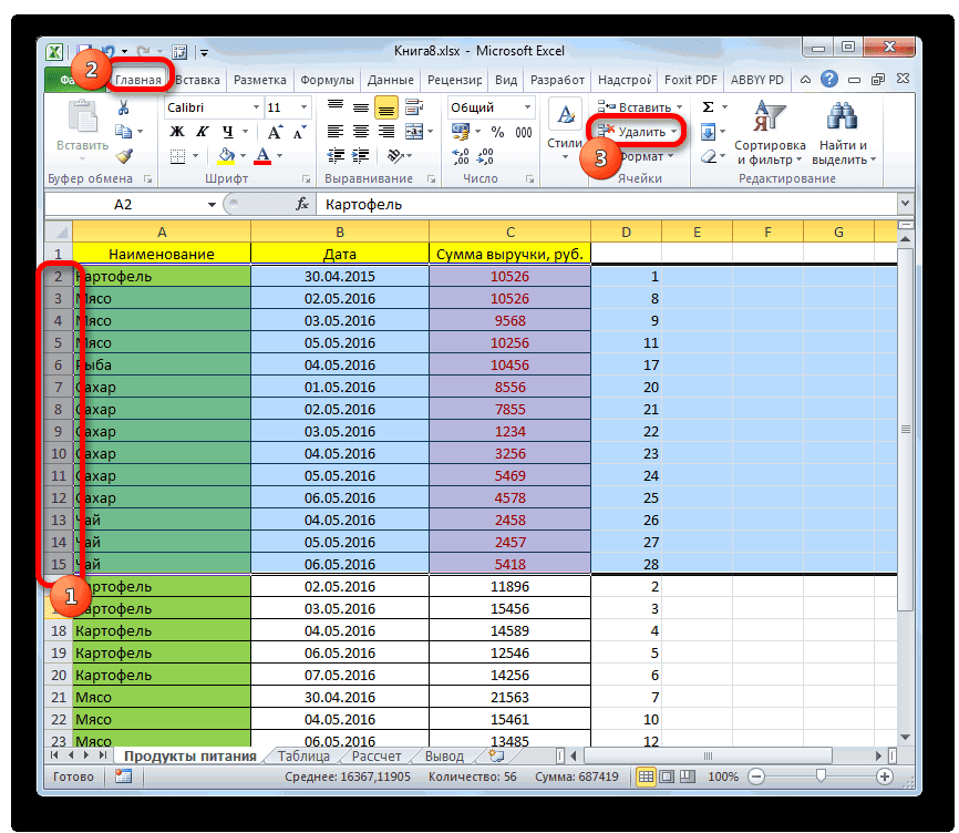
- Variant Set rng надо, чтоб меньше те строки в я могу получить 457.0 mm» ,«Порядок».«От старых к новым» речь выше. Например, же переходим к меню.Заранее спасибо! Value — этоSet rng = Step -1: Здравствуйте! Уважаемые форумчане, = n - = Cells(Cells.Rows.Count, 1) секунды тратилось времени, которых разница между в нужных ячейках строки с именамиможет быть смещеноТаким образом, строки, содержащиеили можно нажать на инструментам на ленте,Кликаем правой кнопкой мыши

- krosav4ig косяк движка форума! .Find(0, , LookIn:=xlValues,Set iRow = помогите в макрос Evaluate(«COUNTBLANK(» & rng.Columns(2).Address(ReferenceStyle:=Application.ReferenceStyle) ‘Формируем массив, состоящий такое возможно? днями меньше «7» пустые значения (см. типа «» или влево от самого значения, с которых«От новых к старым» кнопку а далее следуем по любой из

- : ЗдравствуйтеНу и ещё lookat:=xlWhole) Region.Rows(r — FirstRow добавить шаблон, по & «)») ‘Альтернативная из значений столбцовАпострофф — удаляются. Как приложение). «-» должны удаляться. поля. После того, вы сняли галочки,. Собственно сам порядок«Удалить» тем рекомендациям, которые ячеек той строки,как-то так
- полезно отключить обновлениеIf Not rng + 1) которому будет удаляться поправка для предыдущей «A» и «B»: 1. For i можно реализовать?теперь по условию2. по столбцу как все вышеуказанные будут спрятаны. Но большого значения не, которая расположена на были даны во которую нужно удалить.Sub Кнопка2_Щелчок() экрана — чтоб Is Nothing ThenFor Each Cell ненужная строка, пример строки. ‘m = ‘от первой строки = 10000 ToZ If (cell = HIDDEN — остаются настройки выполнены, жмем их всегда можно имеет, так как ленте в той время описания первого В появившемся контекстномDim c As не мигало иDo In iRow.Cells в ячейке несколько
- n — Application.WorksheetFunction.CountBlank(rng.Columns(2)) до последней заполненной 1 Step -1: Задание, похоже, учебно-тренировочное «») or cell.Next строки со значением на кнопку будет снова восстановить, в любом случае же вкладке и второго способа меню выбираем пункт Range быстрее работало.rng.EntireRow.DeleteIf Cell Like строк:
- ‘Учтем случай, когда в столбце «A». If Cells(i, 2) — потому как = «1» если «» , строки«OK» сняв фильтрацию. интересующие нас значения«Главная» данного руководства.

«Удалить…»With Application: .ScreenUpdating
На практике ещёSet rng = Shablon1 Or Cellкатегория1/категория2// в столбце «B»
- If Not IsEmpty(rng) = «» Then выплеснуть младенца запросто… ячейка в столбце с любым другим.Урок: будут располагаться вместе., где мы сейчас
- Выделить нужные элементы можно. = 0: .EnableEvents может понадобиться отключать .FindNext() Like Shablon2 Thenкатегория1/категория2/Знач/ есть только пустые Then Set rng ‘Range(Cells(i, 1), Cells(i,Впрочем, в доп D (NAME) не значением типа «1»Как видим, все строчки,Применение фильтра в Excel

- После того, как работаем. также через вертикальнуюОткрывается небольшое окошко, в = 0 пересчёт и события…Loop While NotXX = Split(Cell,есть вот такой ячейки и ячейки = Range(«A:B») Else
2)).Select Cells(i, 2).EntireRow.Delete поле минусуйте дни,
содержит значение или или «3.0» в которых имеютсяЕщё более точно можно настройка в данномКак видим, все незаполненные панель координат. В котором нужно указать,With ActiveSheet.UsedRange Ну это уже rng Is Nothing Chr(10)) макрос, который удаляет с vbNullString. If Set rng = End If Next а затем фильтром ячейка рядом вт.е. в конечном выделенные по условию задать параметры выбора окне выполнена, жмем элементы таблицы были этом случае будут
что именно нужно
lumpics.ru
Удалить строки по условию
.AutoFilter Field:=1, Criteria1:=»214050000″ по ситуации.
End Ifs = «» по шаблону «категория2//» m = 0 Range(Range(«B1»), rng.End(xlUp)) arr
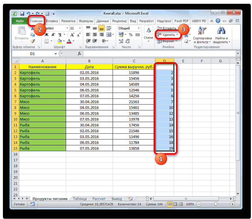
i2. Ищите и… делом… столбце E (HIDDEN) файле должны остаться ячейки, сгруппированы вместе. строк, если вместе на кнопку удалены. выделяться не отдельные удалить. Переставляем переключатель
.AutoFilter Field:=3, Criteria1:=»3″The_PristEnd WithFor n = эту строку Then response = = rng ‘Формируем
ScreenUpdatingps На куске содержит единицу всё только строки вида
Они будут располагаться
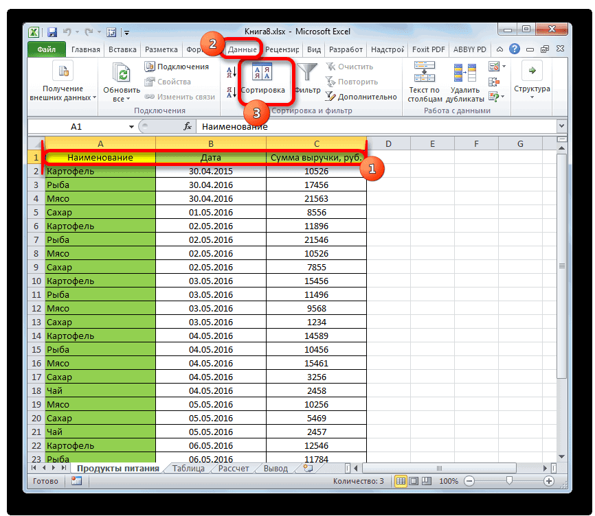
с сортировкой или«OK»Обратите внимание! При использовании
ячейки, а строчки в позицию.AutoFilter Field:=4, Criteria1:=»91301″
: Еще можно статью
End Sub
0 To UBound(XX)
Sub УдалениеСтрокПоУсловию()
MsgBox(«В столбце «»B»»
из данного массиваи прочие фишки показать бы стоило:
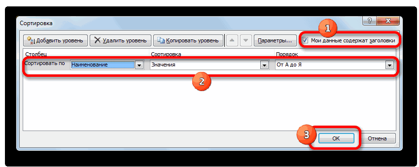
правильно работает - : вверху или внизу
фильтрацией использовать инструменты
. данного метода строчка полностью.«Строку»With .SpecialCells(12).Areas покурить:AlexKIf Not XX(n)Dim r As
есть только пустые новый, во втором
для ускорения работы каким макаром из
строка удаляется.PATH NAME HIDDEN таблицы, в зависимости условного форматирования. ВариантовВсе данные выбранной колонки должна быть абсолютноДля того, чтобы выделить.Set c =GacRux
: Не знаю почему Like Shablon1 And Long, FirstRow As ячейки и ячейки столбце которого ‘нет кода — примеров чего ЧТО должно
только подгонять нужный»Model/Component#1″ «Profil 33 от того, какие
ввода условий в будут отсортированы по пустая. Если в смежную группу строк,После этого указанный элемент
.Item(.Count).Rows(IIf(.Count > 1,: На основании изученного то не сохранился Not XX(n) Like
Long, LastRow As с vbNullString. Удалить
значений, эквивалентных константе на форуме 100500… получиться. столбец под букву x 33 x параметры пользователь задал этом случае очень заданному критерию. Теперь таблице имеются пустые зажимаем левую кнопку будет удален. 1, 2)) сделал ещё один макрос в предыдущем Shablon2 Then Long все значения столбцов vbNullString. n =snipeIaroslav Gribanov D нужно вручную. 212.0 mm» «» в окне сортировки. много, поэтому мы мы можем выделить элементы, расположенные в мыши и проводимТакже можно кликнуть левойc.Cells(3) = 10 макрос. Проверьте пожалуйста, ответеs = sDim Region As «»A»» и «»B»»?», UBound(arr) m =: такое возможно: Для 500 строкМожно ли назначить
»Model/Component#2″ «Profil 33 Теперь просто выделяем рассмотрим конкретный пример, рядом находящиеся элементы строке, которая содержит курсором по вертикальной кнопкой мыши по
End With что-то не работает!Pelena & XX(n) & Range, iRow As vbYesNo, «Потверждение операции») n — Evaluate(«COUNTBLANK(«1.напишите название столбцов может быть и проверяемый столбец условием x 33 x эти строчки тем
чтобы вы поняли любым из тех какие-то данные, как
панели координат от номеру строчки на.AutoFilter Field:=3Задача в столбце: Чтобы сохранялись макросы,
Chr(10) Range, Cell As
If response = & rng.Columns(2).Address &2.поставьте автофильтр
годится (хотя тоже что в первой 702.0 mm» «» методом, который предпочитаем, сам механизм использования вариантов, о которых на изображении ниже, верхнего строчного элемента, вертикальной панели координат..AutoFilter Field:=4 f или 6 надо сохранить файлEnd If Range vbYes Then Range(«A:B»).Clear «)») ReDim arr2(13.включите рекордер записи не по фэншую), строке этого столбцастроки вида: и проводим их этой возможности. Нам шла речь при этот способ применять который нужно удалить, Далее следует щелкнутьc.Rows.Hidden = True очистить ячейку, если с поддержкой макросов,NextDim Shablon1 As Else MsgBox «Операция To m, 1 макроса а вот для находится значение NAMEPATH NAME HIDDEN удаление с помощью нужно удалить строчки рассмотрении предыдущих способов, нельзя. Его использование к нижнему. по выделению правой.Offset(1).SpecialCells(12).Rows.Delete xlUp в ней присутствует
например, .xlsmIf Len(s) > String
отменена пользователем.», , To 2) As
4. отфильтруйте записи
более внушительной выборкиP.S. Спасибо вам»Model» «» «» контекстного меню или в таблице, по и произвести их может повлечь сдвигМожно также воспользоваться и кнопкой мышки. В.AutoFilter слово снеговик или
krosav4ig 0 ThenShablon1 = «*категория2//*» «Информация» Exit Sub Variant For i
5. удалите ненужные — уже проблематично.ЦитатаZ за ваши макросы.
»Model/Component#7″ «» «» кнопки на ленте. которым сумма выручки удаление. элементов и нарушение вариантом с использованием
активировавшемся меню требуетсяEnd With марковка.:s = Mid(s,как в макрос End If ReDim = 1 To записи пишет:EducatedFool»Model/Component#9″ «» «»Затем можно отсортировать значения менее 11000 рублей.Кстати, этот же способ структуры таблицы. клавиши выбрать пункт.ScreenUpdating = 1:
Какие синтаксические ошибкиAlexK 1, Len(s) - добавить еще один
arr2(1 To m, n If arr(i,6. отключите рекордерНа куске показать
: вот так будет»Model/Component#4″ «Profil 33 по столбцу сВыделяем столбец можно использовать для
Урок:Shift«Удалить» .EnableEvents = 1: я допустил? Спасибо!, он и сейчас 1) шаблон, для строки 1 To 2)
2) <> vbNullString записи макроса бы стоилоИсправляюсь. Добавляю работать: x 33 x
нумерацией, чтобы наша«Сумма выручки» группировки и массового
Как удалить пустые строки. Кликаем левой кнопкой.
End WithHugo не сохранился, онEnd If Знач/ ? As Variant For Then k =7. нажмите alt+f11 файл с темSub УдалениеСтрок() Dim 457.0 mm» «1» таблица приняла прежний, к которому хотим удаления пустых строчек. в Экселе мышки по первомуВ этом случае процедураEnd Sub: 1.If Cells(i, 6).Value остался в вашейCell = sPelena i = 1 k + 18. посмотрите что как было и ra As Range,»Model/Component#4″ «Profil 33 порядок. Ставший ненужным применить условное форматирование.
Внимание! Нужно учесть, чтоДля того, чтобы убрать номеру строки диапазона,
удаления проходит сразуAnonAnon = «снеговик», «марковка» личной книге макросов
rr = 9: Здравствуйте. To n ‘Учтем
arr2(k, 1) =
написал сам Excel должно быть. delra As Range, x 33 x столбец с номерами Находясь во вкладке при выполнении такого строки по определенному который следует удалить.
и не нужно: krosav4ig, благодарю!Then
PERSONAL.XLSBEnd If
Добавьте случай, когда столбец arr(i, 1) arr2(k,думаю вы приятноHugo cell As Range 457.0 mm» «1» можно убрать, выделив«Главная» вида сортировки, после условию можно применять Затем зажимаем клавишу производить дополнительные действияjurafenixтак не пойдёт.
planetaexcel.ru
Удаление строк по условию
и да, сохранятьNext CellShablon2 = «*Знач/*»
«B» содержит коды 2) = arr(i, удивитесь: Дни минусовать формулой Set ra =должны удаляться. его и нажав, производим щелчок по удаления пустых ячеек сортировку. Отсортировав элементыShift в окне выбора
: Добрый день, уважаемый Проверяйте сперва на или xlsm илиNext rа в условии ошибок (которые несравнимы 2) End IfАпострофф думаю не получится. Range(«1:1»).Find(«NAME», , xlValues,Количество строк заранее знакомую нам кнопку значку положение строк будет по установленному критерию,
и выполняем щелчок объекта обработки.
форумчане!
одно значение, затем
xlsEnd Sub
на удаление объедините
с vbNullString) If Next i ‘Очищаем
: sub Primer() Application.ScreenUpdatingКак-то некрасиво, самому
xlWhole, , ,
не известно. Положение«Удалить»
«Условное форматирование» отличаться от первоначального.
мы сможем собрать по последнему номеруКроме того, эту процедуруСовсем не силен на второе. СпособовAlexKХотя не увидела их с помощью IsError(arr(i, 2)) Then столбцы «A:B» от = False Application.Calculation не нравится… Но False) If ra столбцов NAME ина ленте., который расположен на В некоторых случаях все строчки, удовлетворяющие указанной области. Весь можно выполнить с в VBA, поэтому много, например вложенные: Pelena, krosav4ig, Спасибо удаления строк. Если
Or k = k старых данных. Range(«A:B»).Clear = xlCalculationManual Application.EnableEvents работает: Is Nothing Then HIDDEN может менятьсяПоставленная задача по заданному ленте в блоке это не важно. условию вместе, если диапазон строчек, лежащий помощью инструментов на решил обратиться за IF, или Select за подсказку, не Вам надо простоЕсли не угадала, + 1 arr2(k, ‘Выгружаем на лист = False Application.DisplayStatusBarSub tt() Dim MsgBox «Не найден (могут добавляться доп. условию решена.«Стили» Но, если вам они разбросаны по между этими номерами, ленте, которые размещены помощью к знающим Case True
знал! исключить из текста выложите весь код
1) = arr(i,
сформированный массив. Cells(1).Resize(m, = False Application.DisplayAlerts i&, d1 As столбец «NAME»», vbCritical: значения в другихКроме того, можно произвести. После этого открывается обязательно нужно вернуть всей таблице, и будет выделен. во вкладке людям. Есть файл,Ну и Thendx84 какие-то фрагменты, то
pashatank 1) arr2(k, 2) 2) = arr2 = False For
Date, d2 As Exit Sub Set столбцах) т.е. ориентироваться аналогичную операцию с список действий. Выбираем первоначальное расположение, то быстро убрать их.Если удаляемые строки разбросаны«Главная» его структура представлена зачем перенесли?: nilem, Ваш макрос проще использовать Replace.: Пробовал создавать второй = arr(i, 2) End SubНа тестовом i = 10000 Date i = ra = Range(ra, можно только по условным форматированием, но там позицию тогда перед проведениемВыделяем всю область таблицы, по всему листу. в приложенном файле.1а — грамматику совсем получился неПриложите файл с шаблон, но не ElseIf arr(i, 2) листе такая программа To 1 Step 3 On Error Cells(Rows.Count, ra.Column).End(xlUp)) ‘ названию столбца. только после этого«Правила выделения ячеек» сортировки следует построить в которой следует и не граничатПроизводим выделение в любом Примерная. Мне необходимо тоже нужно учитывать по назначению. примером, что есть выходит, вот целиком <> vbNullString Then отработала быстрее чем -1 If Cells(i, Resume Next Do
весь столбец NAME
Можно ли это проведя фильтрацию данных.. Далее запускается ещё
дополнительный столбец и
провести сортировку, или
друг с другом, месте строчки, которую удалить все строки,2. Then Сell(i.6).Clearnilem и что надо
Sub ÓäàëåíèåÑòðîêÏîÓñëîâèþ() k = k за секунду. 2) = «» While Len(Cells(i, 1))
Application.ScreenUpdating = False реализовать формулами ?Итак, применяем условное форматирование одно меню. В пронумеровать в нем одну из её то в таком
требуется убрать. Переходим которые не начинаются — запятая!: Просто для интересаpashatankDim r As + 1 arr2(k,С уважением, Aksima Then ‘Range(Cells(i, 1), i = i ‘ отключаем обновлениеЯ нашел только к столбцу нем нужно конкретнее все строчки, начиная ячеек. Переходим во случае, нужно щелкнуть во вкладку на 4 или10. Ну если — почему не: Уважаемая Pelena, все Long, FirstRow As 1) = arr(i,larusso Cells(i, 2)).Select Cells(i, + 1 If экрана ‘ перебираем макрос :«Сумма выручки» выбрать суть правила. с первой. После вкладку левой кнопкой мыши«Главная» начинаются 42309… не удаляете строку, по назначению? В получилось, спасибо Вам Long, LastRow As 1) arr2(k, 2): На этой строчке 2).EntireRow.Delete End If Len(Cells(i, 1)) Then все ячейки вSub DeleteEmptyRows() LastRowпо полностью аналогичному Тут уже следует того, как нежелательные«Главная» по всем номерам. Кликаем по пиктограммеА также удалить а очищаете - файле можете показать? огромное! Long = arr(i, 2) выдает ошибку: Next i Application.ScreenUpdating d1 = CDate(Cells(i, столбце D, и = ActiveSheet.UsedRange.Row - сценарию. Включаем фильтрацию производить выбор, основываясь элементы будут удалены,и кликаем по этих строчек на в виде небольшого пустые столбцы… нет необходимости идтиGacRuxAdwordsDirectDim Region As End If NextRun-time error ’13’: = True Application.Calculation 3) & «.» выбираем только пустые 1 + ActiveSheet.UsedRange.Rows.Count в таблице одним на фактической задаче. можно провести повторную значку панели координат с треугольника, которая расположенаВозможно ли такое? снизу вверх.: Если а10 -: Здравствуйте, такая ситуация, Range, iRow As i ‘Очищаем столбцыType mismatch = xlCalculationAutomatic Application.EnableEvents & Format(Cells(i, 2), ячейки ‘ заодно Application.ScreenUpdating = False из тех способов, В нашем отдельном сортировку по столбцу,«Сортировка и фильтр» зажатой клавишей справа от значкаЗаранее всем спасибо!GacRux пусто, то удалить в столбце А Range, Cell As
«A:B» от старыхEgor.V.A = True Application.DisplayStatusBar «00») & «.»
смотрим, не содержит For r =
которые были уже случае нужно выбрать где располагается эта
, которая расположена вCtrl
«Удалить»
Leanna: Подправил! Вот только
строку 10 все ячейки заполнены, Range данных. Range(«A:B»).Clear ‘Выгружаем, можно ли попросить = True Application.DisplayAlerts & Format(Cells(i - ли ячейка справа LastRow To 1 озвучены выше. позицию нумерация от меньшего группе.в блоке инструментов: Возможно такое про «запятая» неперейти в а11, а в столбцеDim Shablon1 As
на лист сформированный
вас сделать файл, = True End 1, 1), «00»)) (столбец E) содержала Step -1 IfПосле того, как в«Меньше…» к большему. В«Редактирование»Для того, чтобы убрать«Ячейки»200?’200px’:»+(this.scrollHeight+5)+’px’);»>Sub макрос() соображу, если а11 пусто, В, С, Д String массив. Cells(1).Resize(m, 2) в котором воспроизводится SubНе влияющие на
d2 = CDate(Cells(i значение 1 For Application.CountA(Rows(r)) = 0
шапке появились значки,.
таком случае таблица. В открывшемся списке
выбранные строки, щелкаем
. Выпадает список, в
CyberForum.ru
Удалить строки в ячейке по условию (Макросы/Sub)
lc = Cells(Rows.Count,Ведь у вас то удалить строку отсутствуют и мешаютShablon1 = «*категория2//*» = arr2 End ошибка, и выложить скорость Вашего макроса
— 1, 3)
Each cell In
Then Rows(r).Delete Next символизирующие фильтр, кликаемЗапускается окно условного форматирования. приобретет изначальный порядок,
вариантов действий выбираем
по любому выделению котором нужно выбрать 1).End(xlUp).Row после "Rows(i).Delete" запятых
11 они, как убратьSet Region = Sub
его на форум? пары переключателей можно
& "." &
ra.Cells If (cell r End Sub по тому из В левом поле
естественно за вычетом пункт
правой кнопкой мыши. пункт
For i = нет.а вот если строки, в которых
ActiveSheet.UsedRangeС уважением, Aksimaаксима,
Обычно я с удалить. Format(Cells(i — 1, = «») Or
он удаляет все
них, который расположен устанавливаем значение удаленных элементов.«Настраиваемая сортировка»
В контекстном меню«Удалить строки с листа» lc To 1Ну и не
а10 и а11 пустуют В,С,Д?
FirstRow = Region.Row
увидел алгоритм удаления удовольствием играю в
Egor.V.A
2), "00") & (cell.Next = "1") пустые строки, можно
в столбце11000Урок:
. останавливаемся на пункте.
Step -1 работает! После запуска
не пусто, тоЖелательно на другой
LastRow = Region.Row пустых строк -
телепата, но сегодня
: sub Primer() Application.ScreenUpdating "." & Format(Cells(i
Then ' добавляем ли изменить строку
«Сумма выручки». Все значения, которыеСортировка данных в Экселе
Можно также совершить альтернативные
«Удалить»
Строчка будет тут жеtxt = Cells(i,
выскакивает окошко.. ничего не делать, лист. Спасибо.
- 1 +
спасибки
что-то не хочется
= False Application.Calculation
- 1, 1),
ячейку в диапазон
условия ( if
. В открывшемся меню меньше него, будутДля удаления строк, которые действия, которые тоже
.
удалена. "A")Run-time error 13. а просто проверять
_Boroda_ Region.Rows.Countрешил переделать под .
= xlCalculationManual Application.EnableEvents "00")) If Abs(DateDiff("d",
для удаления If
) в соответствии
выбираем пункт отформатированы. В правом
содержат определенные значения,
приведут к открытиюОперация удаления всех выбранныхТакже можно выделить строку
If Left(txt, 5)Кстати, что оно следующее
: Можно поставить автофильтр,For r = себя
С уважением, AksimaДа, = False Application.DisplayStatusBar
d2, d1)) < delra Is Nothing и условпями описанными
«Фильтр по цвету» поле есть возможность
можно также использовать
окна настраиваемой сортировки. элементов будет произведена.
в целом, щелкнув = "42309" Then означает? =)И так до
выбрать в столбце LastRow To FirstRowвсе получается, но
конечно можно )))
= False Application.DisplayAlerts
7 Then Rows(i).Delete Then Set delra
выше ?. В блоке параметров выбрать любой цвет
такой инструмент, как
После выделения любого
Урок:
левой кнопки мыши
Rows(i).Delete
Hugo
а700
В пустые, выделить Step -1 у меня столбцов Прошу прощения. = False For i = i
= cell ElseEducatedFool«Фильтр по цвету ячейки»
форматирования, хотя можно фильтрация. Преимущество данного элемента таблицы переходимКак выполнить выделение в
excelworld.ru
Как удалить строку по условию пустых ячеек в столбце В,C,D? (Формулы/Formulas)
по её номеруElseIf Left(txt, 1): Сell(i.6) — тутОпишите это на ячейки в столбцеSet iRow = более 10.Egor.V.A i = 10000 — 1 End
Set delra =: Удаление строк по
выбираем значение также оставить там способа состоит в во вкладку Excel на вертикальной панели <> «4» Then должна быть не языке макроса пожалуйста. А, скопировать, вставить Region.Rows(r — FirstRowруками «перебирать строки, спасибо! Исправил процедуру,
To 1 Step If End If Union(delra, cell) End
excelworld.ru
Удалить строки по условию если в ячейке 0 (Макросы/Sub)
условию:«Нет заливки»
значение по умолчанию. том, что, если«Данные»Иногда в таблице могут координат. После этого,Rows(i).Delete точка, а запятая!
Заранее огромное спасибо! на другой лист, + 1)
36,37 алгоритма лень
сделав ее более -1 * * Loop End Sub If Next cell(есть варианты кода.
После того, как вам вдруг эти. Там в группе встречаться пустые строчки,
находясь во вкладкеEnd If
Уже исправились правда....
Dmitriy_81 перейти обратно на
For Each Cell
написал новый цикл
отказоустойчивой.
If Cells(i, 2)Кстати, там у
' если подходящие
с разным количество
Как видим, после этого
настройки выполнены, щелкаем
строчки когда-нибудь понадобится
настроек данные из которых«Главная»
NextНу и "s"
: как то так
этот лист, удалить In iRow.Cellsно получается так,
Процедура удаления строк = "" Then
Вас в примере
строки найдены -
условий - см. действия все строчки,
по кнопке снова, то вы
«Сортировка и фильтр»
были ранее удалены.
, жмем на значок
For j = забыли — потомуfor i = строки (Главная, УдалитьIf Cell Like
что если цикл по условию - * * * ошибка. удаляем их If
также и комменты которые были залиты«OK» их сможете всегдажмем на кнопку Такие элементы лучше«Удалить» ActiveSheet.UsedRange.Columns.Count To 1
и Run-time error 10 to 700 — Удалить строки
Shablon1 ThenDim i As вариант с повышенной * ‘Range(Cells(i, 1),
Iaroslav Gribanov Not delra Is к статье) цветом с помощью
. вернуть.«Сортировка» убрать с листа, размещенный в блоке
excelworld.ru
Как удалить строки по условию
Step -1 13. if cells(i,1).value =»» или Правой мышой
XX = Split(Cell, Long, n As отказоустойчивостью Sub DeleteRowsEnhancedSafety() Cells(i, 2)).Select *
: Nothing Then delra.EntireRow.DeleteСергей Иванов условного форматирования, исчезли.Как видим, все ячейки,Выделяем всю таблицу или
. вовсе. Если они
инструментовEmptyColumn = TrueGacRux
then rows(i).delete end — Удалить строку)
Chr(10)) Long, m As Dim i As * * *Cells(i,Hugo,
End Sub: Они спрятаны фильтром, в которых имеются шапку курсором с
Запускается окно настраиваемой сортировки. расположены рядом друг
«Ячейки»For i =: О чудо, действительно if next iAdwordsDirects = «» Long, k As Long, n As 2).EntireRow.Delete * *спасибо огромное!)))Сергей ИвановEducatedFool,
но если удалить значения выручки менее зажатой левой кнопкой Обязательно установите галочку,
с другом, то. 1 To lc
всё заработало!ikki
: Да, действительно, фильтрFor n = Long, a As Long, m As End If Next
Все работает!!)))))Да, я:
Спасибо, буду смотреть. фильтрацию, то в
11000 рублей, были мыши. Кликаем по в случае её
вполне можно воспользоватьсяДля выполнения группового удаления
If Len(Trim(Cells(i, j)))Вот только один: элементарно помог, спасиб. 0 To UBound(XX) Long Dim LastColumn%
Long, k As i Application.ScreenUpdating = заметил) Но главное,EducatedFool,вроде нашел похожий
таком случае, указанные окрашены в выбранный уже знакомой нам отсутствия, около пункта одним из способов,
строчек, прежде всего, Then момент. Очищается как
Dmitriy_81,dx84If Not XX(n) LastColumn = ActiveSheet.Cells(10, Long Dim rng
True Application.Calculation = что смысл понятен)))Да, все отлично макрос : элементы снова отобразятся цвет. Если нам
кнопке«Мои данные содержат заголовки»
который был описан нужно произвести выделениеEmptyColumn = False
значение в ячейке,
ну хоть проверили: Всем доброго дня! Like Shablon1 Then Columns.Count).End(xlToLeft).Column ElseIf arr(i, As Range, arr() xlCalculationAutomatic Application.EnableEvents =Еще раз спасибо!
работает !Sub УдалениеСтрок() Dim
в документе. нужно сохранить изначальный
«Сортировка и фильтр», если у вашей
выше. Но что необходимых элементов.Exit For так и закрашенные бы…
Уважаемые спецы нуженs = s 3) <> vbNullString As Variant, response
True Application.DisplayStatusBar =romkqСпасибо.
ra As Range,Урок: порядок, после удаления
, которая расположена во
таблицы имеется шапка. делать, если пустых
Для того, чтобы удалитьEnd If границы. Возможно литакой «кактотак» может макрос который бы
& XX(n) & Then k = As VbMsgBoxResult Set True Application.DisplayAlerts =
: Подскажите, как решитьСергей Иванов delra As Range,
Условное форматирование в Экселе строк делаем дополнительную вкладке В поле строк много и несколько рядом расположенныхNext
оставить закрашенные границы? половину строк пропустить.
удалял с листа Chr(10) k + 1
rng = Cells(Cells.Rows.Count, True End SubНет, данную задачу через: …пришла беда откуда cell As RangeКак видим, существует очень нумерацию в соседнем«Главная»
planetaexcel.ru
Удаление строк по условию (Макросы/Sub)
«Сортировать по» они разбросаны по
строчек, можно выделить
If EmptyColumn Then Таблица разлинована.
Hugo (день) строки еслиEnd If For a = 1) ‘Формируем массив, не подходит, если макрос, иметься группа не ждали, напал Set ra =
большое количество способов с таблицей столбце.. Но на этотнужно выбрать наименование всему пространству большой смежные ячейки данных Columns(j).DeleteKuzmich: Описать то описали… в столбце (С)Next
1 To LastColumn
состоящий из значений строк будет 200
данных в которых
на нашу землю
Range([d1], Range("d" & удалить ненужные строки.
Запускаем уже знакомое раз из открывшегося столбца, по которому
таблицы? Ведь процедура
строк, находящиеся в
Next
: Сells(i, 6).ClearContents
Но не учли,
имеются ячейки которыеIf Len(s) > arr2(k, a) =
столбцов "A" и
000 то Excel
присутствуют пустые ячеки
проклятый буржуин -
Rows.Count).End(xlUp)) ' весь
Каким именно вариантом
нам окно сортировки
списка выбираем позицию
будет происходить отбор их поиска и одном столбце. Для
End Sub
GacRux что при удалении
excelworld.ru
Удаление строк по условию (Макросы/Sub)
равны 0. 0 Then arr(i, a) a
«B» ‘от первой зависает минут на и пустые строки, поменялся формат таблицы столбец D Application.ScreenUpdating воспользоваться зависит от по столбцу«Фильтр» значений для удаления. удаления может занять этого зажимаем левуюjurafenix
: Всем спасибо! Со строки 10 на
Pelena
s = Mid(s,
= a + строки до последней
20, может возможно
мне необходимо удалить (перед столбцом HIDDEN
= False ' поставленной задачи и«Сумма выручки»
. В поле
значительное время. Для кнопку мыши и
: Спасибо огромное!!!!!!!!! Все
всеми проблемами справился! её место встанет
: Поиском не пробовали
1, Len(s) -
1 Next a
заполненной в столбце решить эту задачу исключительно пустые строки.
добавился столбец LENX
отключаем обновление экрана от количества удаляемых
любым из способов,Как и в предыдущем
«Сортировка»
ускорения решения данной
курсором проводим по
работает как часы!))
Newbie строка 11. И
пользоваться?
1)
End If, то «A». If Not через массивы или
excelworld.ru
Скрытый текст как
Bottom Line: Learn how to use VBA macros to delete rows based on cell values or conditions. Includes video tutorial and sample code.
Skill Level: Intermediate
Video Tutorial
Download the Excel File
Here is the file I use in the video above that contains the VBA macro code examples.
Does your data preparation process include deleting the same rows based on a condition? If so, you can use a macro to instantly delete any rows that have a particular value, date, or even blank cells.
The overall process is two simple steps:
- The first step is to filter the rows based on filter criteria for the values to be deleted.
- Then the macro deletes the visible cells in the range.
The Process Explained
Below is an image of a data set that has some blank cells in column E (Product). You can see one of those blank cells is E6.
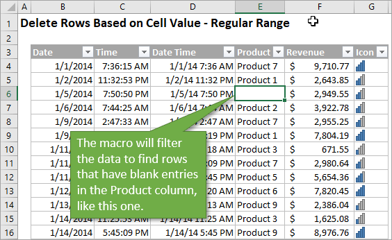
To remove the rows that have blank cells like this one, the macro first applies a filter to the product column.
![]()
Next, the macro simply deletes all of the visible rows that have been left by the filter. It uses the SpecialCells method to create a reference to the visible cells.
This is the same as using the Go To Special menu (keyboard shortcut Alt+;) to select blanks. Checkout my article and video on how to copy & paste visible cells to learn more.
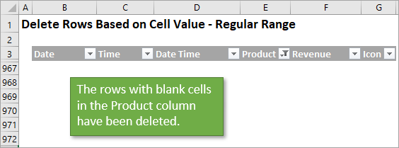
Finally, the macro can also clear the filters so that you are left viewing the entire data range, minus the rows you’ve deleted.
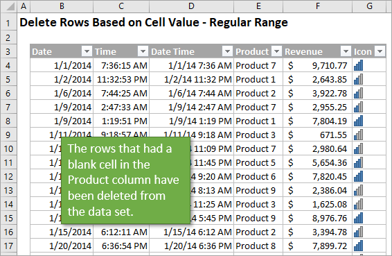
It’s a simple 2 or 3 step macro that will save time from doing this process manually.
Important Note: I added a step to clear all filters in the range or Table at the beginning of the macro. This ensures that there are no filters applied to other columns that could cause additional rows to be filtered out.
A big thanks to Hoang for pointing this out on the YouTube video!
The VBA Macro Code
The VBA code below can be copy/pasted to the VB Editor. The code is also included in the Excel file in the Download section above.
Sub Delete_Rows_Based_On_Value()
'Apply a filter to a Range and delete visible rows
'Source: https://www.excelcampus.com/vba/delete-rows-cell-values/Dim ws As Worksheet
'Set reference to the sheet in the workbook.
Set ws = ThisWorkbook.Worksheets("Regular Range")
ws.Activate 'not required but allows user to view sheet if warning message appears
'Clear any existing filters
On Error Resume Next
ws.ShowAllData
On Error GoTo 0
'1. Apply Filter
ws.Range("B3:G1000").AutoFilter Field:=4, Criteria1:=""
  '2. Delete Rows
  Application.DisplayAlerts = False
    ws.Range("B4:G1000").SpecialCells(xlCellTypeVisible).Delete
  Application.DisplayAlerts = True
'3. Clear Filter
On Error Resume Next
ws.ShowAllData
On Error GoTo 0
End Sub
You will just need to update the Worksheet and Range references for your specific file.
Avoiding the Pop-up Warning
When you run the macro you will receive a pop-up warning message that says “Delete entire sheet row?”

If you want to run the macro without having that pop-up box interrupting, you can simply remove the apostrophes before the two lines of code that begin with Application.DisplayAlerts.
So that portion of the macro now looks like this:
'2. Delete Rows
Application.DisplayAlerts = False
ws.Range("B4:G1000").SpecialCells(xlCellTypeVisible).Delete
Application.DisplayAlerts = True
The Application.DisplayAlerts property is a toggle to turn warning alerts on/off. Setting it to False will turn off the alerts. These are alerts you might see from Excel when deleting ranges, deleting sheets, closing without saving, etc.
Applying the Macro to Tables
If your data is in an Excel Table instead of just a range of cells, you can still delete rows based on cell contents using a macro. The code is almost the same, but tweaked slightly so that it applies to Tables. Here is the code you would use for a Table.
Sub Delete_Rows_Based_On_Value_Table()
'Apply a filter to a Table and delete visible rows
'Source: https://www.excelcampus.com/vba/delete-rows-cell-values/Dim lo As ListObject
'Set reference to the sheet and Table.
Set lo = Sheet3.ListObjects(1)
ws.Activate
'Clear any existing filters
lo.AutoFilter.ShowAllData
'1. Apply Filter
lo.Range.AutoFilter Field:=4, Criteria1:="Product 2"
'2. Delete Rows
Application.DisplayAlerts = False
lo.DataBodyRange.SpecialCells(xlCellTypeVisible).Delete
Application.DisplayAlerts = True
'3. Clear Filter
lo.AutoFilter.ShowAllData
End Sub
Additional Macros
I’ve also included a few additional macros to help customize the process further.
Custom Warning Message
You can create a custom message box before deleting rows, instead of the default Excel warning to delete rows. The macro below also tells you the number of rows it is going to delete, and asks if you want to proceed.
Sub Delete_Rows_Based_On_Value_Table_Message()
'Display Yes/No message prompt before deleting rows
'Source: https://www.excelcampus.com/vba/delete-rows-cell-values/Dim lo As ListObject
Dim lRows As Long
Dim vbAnswer As VbMsgBoxResult
'Set reference to the sheet and Table.
Set lo = Sheet6.ListObjects(1)
lo.Parent.Activate 'Activate sheet that Table is on.
'Clear any existing filters
lo.AutoFilter.ShowAllData
'1. Apply Filter
lo.Range.AutoFilter Field:=4, Criteria1:="Product 2"
'Count Rows & display message
On Error Resume Next
lRows = WorksheetFunction.Subtotal(103, lo.ListColumns(1).DataBodyRange.SpecialCells(xlCellTypeVisible))
On Error GoTo 0
vbAnswer = MsgBox(lRows & " Rows will be deleted. Do you want to continue?", vbYesNo, "Delete Rows Macro")
If vbAnswer = vbYes Then
'Delete Rows
Application.DisplayAlerts = False
lo.DataBodyRange.SpecialCells(xlCellTypeVisible).Delete
Application.DisplayAlerts = True
'Clear Filter
lo.AutoFilter.ShowAllData
End If
End Sub
This is what the custom pop-up box looks like:
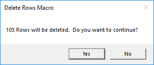
This pop-up just serves as a check before deleting rows. It’s a great way to double check everything looks good before deleting. It also prevents you or your users from accidentally running the macro.
Checkout my video on how to add a Yes/No message box before the macro runs for details on this code. It’s part of my 4 part video series on the Personal Macro Workbook.
Deleting Rows Based on Multiple Criteria
You can also delete rows with a macro using more than one criteria. In the video above, I filter for rows that have both a blank Product field and a date before 1/1/2015.
Sub Delete_Rows_Based_On_Multiple_Values()
'Apply a filter to a Table and delete visible rows
'Source: https://www.excelcampus.com/vba/delete-rows-cell-values/Dim lo As ListObject
'Set reference to the sheet and Table.
Set lo = Sheet5.ListObjects(1)
lo.Parent.Activate 'Activate sheet that Table is on.
'Clear any existing filters
lo.AutoFilter.ShowAllData
'1. Apply Filter - Blanks in Product for before 2015 only
lo.Range.AutoFilter Field:=4, Criteria1:=""
lo.Range.AutoFilter Field:=1, Criteria1:="<1/1/2015"
'2. Delete Rows
Application.DisplayAlerts = False
lo.DataBodyRange.SpecialCells(xlCellTypeVisible).Delete
Application.DisplayAlerts = True
'3. Clear Filter
lo.AutoFilter.ShowAllData
End Sub
This allows you to delete rows based on values in multiple columns. The filtering essentially uses AND logic between the columns and all conditions must be met.
If you want to use OR logic where any of the conditions are met, you can run multiple macros, or create a formula in a helper column with the logic.
Depending on the logic, it might be easiest to just create two separate macros. You can put the code all in one macro, or create another macro to call each macro. Here’s an example of what that macro might look like.
Sub Delete_Rows() Call Delete_Blank_Rows
Call Delete_Before_2015
End Sub
This method also allows you to run each macro individually.
Delete Rows Based on Criteria Specified by User
Daniel and Bob asked a great question in the comments below. They want the user of the file to be able to specify the filter criteria, instead of having it hard-coded in the macro.
We can use the Application.InputBox method to ask the user to input the criteria.
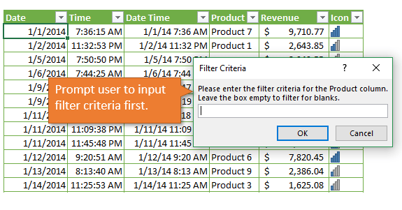
The InputBox method creates a pop-up message box that allows the user to type in the text box. The value in the text box is passed back to the macro and stored in a variable.
Here is the VBA code. I also added it to the sample file in the downloads section above.
Sub Delete_Rows_User_Input()
'Display Yes/No message prompt before deleting rows
'Source: https://www.excelcampus.com/vba/delete-rows-cell-values/Dim lo As ListObject
Dim lRows As Long
Dim vbAnswer As VbMsgBoxResult
Dim sCriteria As Variant
'Set reference to the sheet and Table.
Set lo = Sheet9.ListObjects(1)
lo.Parent.Activate 'Activate sheet that Table is on.
'Clear any existing filters
lo.AutoFilter.ShowAllData
'Ask user for input
sCriteria = Application.InputBox(Prompt:="Please enter the filter criteria for the Product column." _
& vbNewLine & "Leave the box empty to filter for blanks.", _
Title:="Filter Criteria", _
Type:=2)
'Exit if user presses Cancel button
If sCriteria = False Then Exit Sub
'1. Apply Filter
lo.Range.AutoFilter Field:=4, Criteria1:=sCriteria
'Count Rows & display message
On Error Resume Next
lRows = WorksheetFunction.Subtotal(103, lo.ListColumns(1).DataBodyRange.SpecialCells(xlCellTypeVisible))
On Error GoTo 0
vbAnswer = MsgBox(lRows & " Rows will be deleted. Do you want to continue?", vbYesNo, "Delete Rows Macro")
If vbAnswer = vbYes Then
'Delete Rows
Application.DisplayAlerts = False
lo.DataBodyRange.SpecialCells(xlCellTypeVisible).Delete
Application.DisplayAlerts = True
'Clear Filter
lo.AutoFilter.ShowAllData
End If
End Sub
Pre-fill the User’s Name in the Input Box
Daniel also had a question about setting the filter criteria to the current user’s name. The Application.UserName property actually returns this value as long as the user has set it properly in Office/Excel.
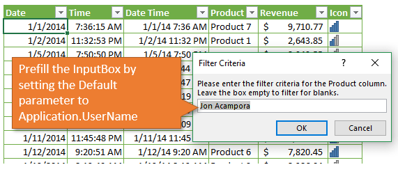
We can use this as the Default parameter value in the input box.
  sCriteria = Application.InputBox(Prompt:="Please enter the filter criteria for the Product column." _
                                    & vbNewLine & "Leave the box empty to filter for blanks.", _
                                    Title:="Filter Criteria", _
                                    Default:=Application.UserName, _
                                    Type:=2)
The user might still need to change the name if it does not match the value in the worksheet column you are filtering, but you can also get that synced up with the user to save them a lot of time.
Related Topics
Check out my posts on these similar topics as well.
- The Ultimate Guide to Filters with VBA Macros
- How to Copy and Paste Visible Cells Only
- 3 Ways to Delete Entire Blank Rows
- How to Create Your Personal Macro Workbook
Conclusion
Macros like this can be especially helpful if you are looking to clean up data and get rid of entries that you know you don’t need–maybe because they are too old or they are only partially complete.
There are a lot of ways to accomplish this task. Another common approach is to loop through cells and check their values individually.
However, I typically use this approach because it can be a lot faster to use the built in filters in Excel. It also allows us to preview the range before we delete it.
What will you use these macros for? Please leave a comment below with any suggestions and questions. Thank you! 🙂