
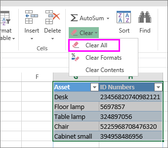
If your Excel worksheet has data in a table format and you no longer want the data and its formatting, here’s how you can remove the entire table. Select all the cells in the table, click Clear and pick Clear All.
Tip: You can also select the table and press Delete.
If you want to keep the data without the table format, you won’t be able to do that in Excel for the web. Learn more about using the Excel desktop application to convert a table to a data range.
Need more help?
Want more options?
Explore subscription benefits, browse training courses, learn how to secure your device, and more.
Communities help you ask and answer questions, give feedback, and hear from experts with rich knowledge.
There are two common ways to delete a table in Excel:
Method 1: Delete Table Without Losing Data
Method 2: Delete Table Including Data
The following examples show how to use each method in practice with the following table in Excel:

Example 1: Delete Table Without Losing Data
To delete a table without actually deleting the data values, first click any cell in the table.
Next, click the Table Design tab along the top ribbon, then click the icon called Convert to Range within the Tools group:

This will convert the table to a normal range of data. However, the format with the alternating blue lines will still be present.
To remove this formatting, highlight each cell in the range A1:C10 and then click the Cell Styles icon in the Styles group on the Home tab. Then click Normal:

The formatting will automatically be removed from the cells:

We have successfully deleted the table without actually deleting the data from the cells.
Example 2: Delete Table Including Data
To delete an entire table including the data, first highlight the entire table range A1:C10, then click the Clear icon within the Editing group on the Home tab.
Then click Clear All from the dropdown menu:

The entire table including the data will be deleted from the Excel sheet:

Additional Resources
The following tutorials explain how to perform other common tasks in Excel:
Excel: How to Delete Rows with Specific Text
Excel: How to Delete Filtered Rows
Excel: How to Delete Calculated Field in Pivot Table
To remove a table but keep data and formatting, go to the Design tab Tools group, and click Convert to Range.
How to remove table formatting
- Select any cell in the table.
- On the Design tab, in the Table Styles group, click the More button.
- Underneath the table style templates, click Clear.
Contents
- 1 How do I delete a table in Excel but keep the data?
- 2 How do I remove a table from Excel?
- 3 How do you delete a data table?
- 4 How do you delete a column in Excel without losing data?
- 5 How do I delete a table without deleting the text?
- 6 How do I make a table in Excel without data?
- 7 How do I remove a table from a data model in Excel?
- 8 What is the shortcut to delete a table in Excel?
- 9 How do I remove table formatting in Excel 2021?
- 10 How do I edit a data table in Excel?
- 11 How do I refresh a data table in Excel?
- 12 What is an Excel data table?
- 13 Can you delete a table in word but keep the text?
- 14 How do you delete a column in Word without losing data?
- 15 Which option is used to delete the table of contents from a document?
- 16 How do I delete rows and records in Excel?
- 17 How do I format Excel nicely?
- 18 How do you delete a data connection in Excel?
- 19 How do I remove a table from a pivot table?
- 20 How do I remove power from pivot table in Excel?
How do I delete a table in Excel but keep the data?
To remove a table:
- Select any cell in your table. The Design tab will appear.
- Click the Convert to Range command in the Tools group. Clicking Convert to Range.
- A dialog box will appear. Click Yes.
- The range will no longer be a table, but the cells will retain their data and formatting.
How do I remove a table from Excel?
Remove a table style. Select any cell in the table from which you want to remove the current table style. On the Home tab, click Format as Table, or expand the Table Styles gallery from the Table Tools > Design tab (the Table tab on a Mac). Click Clear.
How do you delete a data table?
Clear a Data Table
- Select all the cells in the data table, including the heading.
- On the keyboard, press the Delete key.
How do you delete a column in Excel without losing data?
Highlight the columns/range you want to clear, right-click on your mouse, and select Clear Contents.
How do I delete a table without deleting the text?
How to Remove Table without Deleting Text in Microsoft Word
- Click on the table you want to remove.
- Go to the Table Tools > Layout menu.
- Click Convert to Text.
- Select the separator type between text, then click OK.
- The table is now removed and the text still there.
How do I make a table in Excel without data?
Create a table, then convert it back into a Range
- On the worksheet, select a range of cells that you want to format by applying a predefined table style.
- On the Home tab, in the Styles group, click Format as Table.
- Click the table style that you want to use.
- Click anywhere in the table.
How do I remove a table from a data model in Excel?
- Click Home > Diagram View.
- Right-click a relationship line that connects two tables and then click Delete. To select multiple relationships, hold down CTRL while you click each relationship.
- In the warning dialog box, verify that you want to delete the relationship, and then click OK. Notes:
What is the shortcut to delete a table in Excel?
Keyboard shortcut to clear all in Excel Windows is ALT + H + E + A (press these keys one after the other in succession). So these are some scenarios where you can remove table formatting in Excel.
How do I remove table formatting in Excel 2021?
How to clear all formatting in a table
- Click any cell within a table, and then press Ctrl + A twice to select the whole table including the headers.
- On the Home tab, in the Editing group, click Clear > Clear Formats.
How do I edit a data table in Excel?
How to Edit Data Table Properties
- Select Edit > Data Table Properties.
- Click on the data table to use in the Data tables list. Comment: New data tables are added by selecting File > Add Data Tables….
- Click on the Set as Default button to the right of the Data tables list.
- Click OK.
How do I refresh a data table in Excel?
Manually refresh
To update the information to match the data source, click the Refresh button, or press ALT+F5. You can also right-click the PivotTable, and then click Refresh. To refresh all PivotTables in the workbook, click the Refresh button arrow, and then click Refresh All.
What is an Excel data table?
What is a data table in Excel? In Microsoft Excel, a data table is one of the What-If Analysis tools that allows you to try out different input values for formulas and see how changes in those values affect the formulas output.
Can you delete a table in word but keep the text?
Put the cursor inside the table so that the Table Tools>Layout tab of the ribbon is revealed and then click on the Convert To Text button and accept the Separate text with Tabs option and then click on OK.
How do you delete a column in Word without losing data?
Click a column or cell in the table, and then click the Table Layout tab. Under Rows & Columns, click Delete, and then click Delete Columns.
Which option is used to delete the table of contents from a document?
Answer: Click on the References tab and from the Table of Contents group, click Table of Contents. Select Remove Table of Contents from the drop-down menu by clicking on it.
How do I delete rows and records in Excel?
If you don’t need any of the existing cells, rows or columns, here’s how to delete them:
- Select the cells, rows, or columns that you want to delete.
- Right-click, and then select the appropriate delete option, for example, Delete Cells & Shift Up, Delete Cells & Shift Left, Delete Rows, or Delete Columns.
How do I format Excel nicely?
13 Ways to Make your Excel Formatting Look More Pro
- Don’t use column A or row 1.
- Use charts, but avoid 3D charts.
- Images are important.
- Resize rows and columns.
- Don’t use many colors.
- Turn off gridlines and headers, and chart borders.
- Avoid using more than 2 fonts.
- Table of contents.
How do you delete a data connection in Excel?
If you want to remove connections which are connected to the workbook then follow steps below: Excel> data>connections section> connections> Remove whichever is not needed.
How do I remove a table from a pivot table?
Below are the steps to delete the Pivot table as well as any summary data:
- Select any cell in the Pivot Table.
- Click on the ‘Analyze’ tab in the ribbon.
- In the Actions group, click on the ‘Select’ option.
- Click on Entire Pivot table.
- Hit the Delete key.
How do I remove power from pivot table in Excel?
Delete a PivotTable
- Pick a cell anywhere in the PivotTable to show the PivotTable Tools on the ribbon.
- Click Analyze > Select, and then pick Entire PivotTable.
- Press Delete.
(Note: This guide on how to remove tables in Excel is suitable for all Excel versions including Office 365)
In Excel, when you have large amounts of consistent and uniform data sets, converting them to a table paves an easy way to enter, search, and retrieve the data.
When you create a table with the data, Excel automatically adds some formatting of its own. However, there are a variety of formatting options you can use to change the layout of the cell and perform any operations on them. This makes data handling a lot easier.
However, in some cases, you might need to remove the table formatting or even the whole table.
In this article, I will tell you how to remove table formatting in Excel. Additionally, you’ll also see how to remove tables in Excel using 3 easy ways.
You’ll Learn:
- Excel Table and Formatting
- How to Remove Table Formatting in Excel?
- Using Format As Table Option
- How to Remove Tables in Excel?
- Using the Convert to Range Option
- Using the Clear Button
- Using Keyboard Shortcuts
- By Pressing the Delete Key
- By Using the Excel Hotkeys
Watch this Video on How to Remove Tables in Excel in 3 Easy Ways
Related Reads:
How to Create a Pivot Table in Excel? — The Easiest guide
How to Create an Excel Map Chart from Pivot Table Data? 3 Simple Steps
How to Group in Pivot Table? ( 2 Easy Methods)
Excel Table and Formatting
Before we learn how to remove table formatting in Excel, let us take a quick stroll into how a table is created and formatted.
Consider an example where you have the data from different people grouped into different categories like first name, last name, age, state, and country.

This data, however, is simple and you can easily search through it or perform any functions. But what if the data are large in numbers? You will have to use filters to showcase necessary information, sort the data, and perform desired functions.
In these cases, you will convert the normal data called “normal ranged data” into a “table”. An easy way to convert the normal data to a table is by pressing Ctrl + T and in the Create Tables header, select the data and click OK. If your data has headers, check the checkbox for My table has headers and click OK.
If you add any additional data, the present data will be formatted as a table.

You can see the table appears with default formatting. However, you can add additional formatting to the table from the Home or Table Design ribbon.
If you feel like the default formatting does not suit your needs, you can either choose other built-in formats or create and apply custom formats.
If you are still not satisfied with the formatting or the whole table, follow the below-mentioned methods to remove them.
Suggested Reads:
How to Remove Dropdown in Excel? 3 Easy Methods
How to Remove Dotted Lines in Excel? 3 Different Cases
How to Remove Comma in Excel? 5 Easy Ways
How to Remove Table Formatting in Excel?
Let us first see how to remove the table formatting in Excel.
From the above example, you can see the table is formatted with dark blue background headings and alternating light blue and white patterns.
Suppose you want to remove the formatting of the table so that the table appears with the simple default background. For this, you can use this method.
Using Format As Table Option
This is one of the most common methods to remove table format in Excel.
- To remove the table formatting, first, select the table.
- Navigate to Table Design and under the Table Styles section, click on the More dropdown.

- Scroll down and click on Clear from the dropdown.

This only removes the formatting of the table, but the data, filters, and other elements remain in the table format.
- Now, navigate to Home. Under the Editing section, click on the dropdown from Clear and select Clear Formats.
This removes the dropdown from the headers and converts the table to normal range data.

How to Remove Tables in Excel?
In the above-mentioned method, we saw how to remove the formatting in a table. However, in some cases, you might have to delete or remove the whole table.
Let us see 3 ways to remove tables in Excel.
Using the Convert to Range Option
If there is no need for an Excel table, you can easily convert the table to normal data using this method.
- First, select the Excel table that you want to convert to normal data.
- Navigate to Table Design. Under the Tools section, click on Convert to Range.

- You can also right-click on the table and click on the extend option from Table and select Convert to Range.

- Excel throws a warning pop-up asking “Do you want to convert the table to a normal range?”

- Click Yes.
- This instantly converts the table to normal data.

You can see that the dropdown filters and sorting options and structured references are removed. You can also see that, though the table is removed, the formatting style remains. So, before you convert the table to a normal data range, it is always better to remove the table formatting using the above method and then remove the table.
- There is another easy way to remove the formatting in the cells. First, select the cells you want to remove the formatting from.
- Then, navigate to Home. Under the Editing section, click on the dropdown from Clear and select Clear Formats.

This deletes the formatting of the selected cells and turns the data back to the default formatting.
Using the Clear Button
This method acts as a hard reset option. This method can be used when you want to clear the formatting of the cells in addition to the data in the table.
- To clear the table along with the data, first, select the table.
- Navigate to Home. Under the Editing section, click on the dropdown Clear and select Clear All.

- This removes the table including the data and returns the blank cells.

Using Keyboard Shortcuts
If you are a person who uses a keyboard predominantly for efficient functioning, then these are easy methods to remove tables in Excel.
By Pressing the Delete Key
This is a very simple method to remove tables in Excel without many elaborate steps.
- First, select the table either by clicking and dragging the cells or by holding the Shift and arrow keys.
- Then, press the Delete key on the keyboard.
- This instantly deletes the selected data and its formatting.
By Using the Excel Hotkeys
Another method to remove a table in Excel is by using the hotkeys. Hotkeys are a series of keystrokes that you can use to perform certain functions instead of using a mouse.
This method works on the same principle as selecting the Clear All button, but with the help of your keyboard.
- To remove a table, first, select the table.
- Then, while holding the Alt key, press the keys H, E, and A one after the other (Alt + H + E + A).
- This removes the table and all the cells in it.
Also Read:
How to Select Multiple Cells in Excel? 7 Simple Ways
How to Remove Spaces in Excel? 3 Easy Methods
How to Remove Hyperlinks in Excel? 3 Easy Methods
Frequently Asked Questions
How do I convert a table to normal data in Excel without deleting the data?
Select the table. Right-click > Table > Convert to Range or navigate to Table Design > Convert to Range. Click Yes in the pop-up. This removes the table. To remove the formatting, navigate to Home. Under the Editing section, click on the dropdown from Clear and select Clear Formats.
What is the easiest way to delete a table?
Selecting the data and pressing the Delete button is the easiest method to delete a table and its data completely.
How do I remove only the formatting of the table in Excel?
If you only want to remove the formatting of the table in Excel, select the cells you want to remove the formatting and navigate to Home, under the Editing section, click on the dropdown from Clear and click Clear Formats.
Closing Thoughts
Excel offers you the flexibility to change or even remove the formatting of the table to suit your needs. Additionally, you can also delete the whole table depending on your choice.
In this article, we saw how to remove table formatting in Excel the easy way. We also saw how to remove tables in Excel using 4 simple ways. Choose the method that suits your purpose the best.
If you need more high-quality Excel guides, please check out our free Excel resources center. Simon Sez IT has been teaching Excel for over ten years. For a low, monthly fee you can get access to 140+ IT training courses. Click here for advanced Excel courses with in-depth training modules.

Simon Calder

Chris “Simon” Calder was working as a Project Manager in IT for one of Los Angeles’ most prestigious cultural institutions, LACMA.He taught himself to use Microsoft Project from a giant textbook and hated every moment of it. Online learning was in its infancy then, but he spotted an opportunity and made an online MS Project course — the rest, as they say, is history!
In this video, we’ll look at how to remove a table from an Excel worksheet.
In this workbook, we have a number of Excel Tables. Let’s look at some ways you can remove these tables.
You won’t find a «delete table» command in Excel.
To completely remove an Excel table, and all associated data, you’ll want to delete all associated rows and columns.
If a table sits alone on a worksheet, the fastest way is to delete the sheet.
For example, this sheet contains a table showing the busiest airports in the world. When I delete the sheet, the table is completely removed.
If you want to keep the sheet, but delete the table, you can select and delete a range that includes the entire table.
On this sheet, I want to remove the Orders table and leave the summaries.
I’ll select the first column, then hold down the Shift key and select the last. Then I’ll Right-Click and Delete.
In both of these cases, the tables and data are completely removed, and the table names no longer appear in the name box.
Now, if you want to keep all data and just «undefine» an Excel table, use the «convert to range» button on the Design tab of the ribbon.
This command leaves all data and formatting in place, and removes only the table definition.
To illustrate, here I have a table named «movies».
If I place the cursor anywhere in the table, and use «convert to range», the table is removed, but the data and formatting remain.
What happens to formulas that use structured references when you convert a table to a range? Let’s look at an example.
In this table, the Total column is a formula that multiples quantity by price. You can see the formula uses structured references. To the right, another formula counts rows in the table using a structured reference.
When I convert this table to a range, everything keeps working, but the formulas are translated to standard references.
One thing you may find confusing is that table formatting sticks around, even when you convert a table to a range.
If you want to remove table formatting, the simplest way is to set the format to «None» before converting the table to a range.
I’ll undo back to the table, and try that now.
Under Table Styles, I’ll choose the «None» option.
Now when I convert the table to a range, the formatting is already gone, so no trace of the table remains.
Surely you all know the Microsoft Excel application. Microsoft Excel is an application or software that is useful for processing numbers. As you already know, this application has a lot of uses and benefits.
The usefulness of this application is that it can create, analyze, edit, Rank, and sort several data because this application can calculate with arithmetic and statistics.
This tutorial will explain how to sort or rank data using Microsoft Excel.
How to Rank in Microsoft Excel
You can rank data in Microsoft Excel. By using the application, you can easily do work in processing data. Ranking data is also very useful for those who work as teachers.
Because this application can rank data in a very easy way and can be done by everyone. Here are ways to rank data in Microsoft Excel:
1. The first step you can take is to open a Microsoft Excel worksheet that already has the data you want to rank. In the example below, I want to rank students in a class by sorting them from rank 1 to 7 You can also rank according to the data you have.
![]()
2. After that, you can place your cursor in the cell, where you will rank the cells in the first order. You can see an example in the image below.
![]()
After that, you can write a formula to rank in Microsoft Excel in the fx column. And here’s the formula, =rank(number;ref;order) .
The meaning of the formula is = Rank Rank, which means it is a rank function. And (number; ref; order) means the initial cell number that has a value to be ranked, its reference, and the final cell number that has a value to be ranked, the reference.
The formula is =Rank(D3;$D$3:$D$9;0) in the example below. After entering the function, you can press the Enter key on your keyboard. And here are the results, namely the ranking on data number 1, which has a ranking of 1.
![]()
3. If you want to do the same thing to all data as in data number 1, you have to copy the previous column, and then you can block the column below it and click Paste. Then you can see the results. All the columns in the Rank entity have been ranked in such away.
![]()
4. The results above are not satisfactory because the data is still not sorted, so it looks messy. We must make it sequentially according to the ranking from the smallest to the largest, and this example must be sorted from rank 1 to rank 9.
The way to sort it is to block the contents of all tables, but not with the column names and the contents of the column number.
![]()
5. After that, you can do the sorting by going to the Editing tool, clicking Sort & Filter, and then clicking the Custom Sort option…
![]()
6. Then the Sort box will appear, where you have to choose sort by with the Rank option, some kind on with the Values option, and order with the Smallest to Largest option. After that, you can click OK.
7. Below is the result of the sorting we have done above. In this way, the data that has been ranked will be sorted according to its ranking.
![]()
That’s the tutorial on how to rank using Microsoft Excel. Hopefully, this article can be useful for you.
Microsoft Excel Tip: Delete A Table Without Losing The Data or Table Formatting
Microsoft Excel Tip: Delete A Table Without Losing The Data or Table Formatting
|
After you create a table in Microsoft Office Excel, you might not want to keep working with the table functionality that it includes. Or you might want a table style without the
table functionality. To stop working with your data in a table without losing any table style formatting that you applied, you can convert the table to a regular range of data on the worksheet. |
|
|
To successfully complete this procedure, you must have created an Excel table in your worksheet.
Click anywhere in the table. This displays the Table Tools, adding the Design tab.
A cell in the table must be selected for the Design tab to be visible.
On the Design tab, in the Tools group, click Convert to Range.
|
|
Table features are no longer available after you convert the table back to a range.
For example, the row headers no longer include the sort and filter arrows, and structured references (references that use table names) that were used in formulas turn into regular cell references.
|
|
|
*You can also right-click the table, point to Table, and then click Convert to Range.
*Immediately after you create a table, you can also click Undo on the Quick Access Toolbar to convert that table back to a range.
|
Share This Story, Choose Your Platform!
Related Posts
Page load link
What Are Excel Tables?
Tables in Excel are named objects that assist in managing inter-related data in a series of rows and columns, independently, from the remaining spreadsheet data. Moreover, Excel tables offer features that help users manipulate and format their data quickly, thus making it easy for them to work with massive data sets.
For instance, the below cell range shows the revenues of US tech companies from 2018 to 2021.

Using tables in Excel option, we can make the above data range more organized and easy to analyze.

Also, the Excel tables have alternative colored rows with filters in all the columns.
Remember, when we create an Excel table, it automatically assigns names to the table and its columns. As a result, we can see structured references to the cells with AVERAGE() function in the range F2:F6, thus making the formula and the table more readable and easy to grasp.
Table of contents
- What Are Excel Tables?
- How To Make Tables In Excel?
- 1. Using Table Option From Insert tab
- 2. Using Tables In Excel Shortcut
- 3. Using Format As Table Option From Home tab
- How To Customize Tables In Excel?
- 1. Change Excel Table Name
- Naming tables in Excel
- Change Excel Table Color
- 1. Change Excel Table Name
- Useful Features Of Excel Tables
- 1. Sorting And Filtering Options
- 2. Column Headers Visible During Scrolling
- 3. Simple Formatting Steps
- 4. Automatic Table Expansion
- 5. Quick Access To Functions
- 6. Quick Calculations
- 7. Structured References In Excel Table Functions And Formulas
- How To Manage Table Data?
- 1. Converting An Excel Table To A Range
- 2. Inserting and Deleting Table Rows and Columns
- Inserting table rows and columns
- Deleting Table Rows And Columns
- 3. Resizing Excel Table
- 4. Selecting an Excel Table Row or Column
- Selecting table columns
- Selecting table rows
- Selecting the entire table
- 5. Inserting a Slicer for Filtering Table Data
- 6. Removing Duplicates from Excel Table
- Important Things To Note
- Frequently Asked Questions
- Download Template
- Recommended Articles
- How To Make Tables In Excel?
- Tables in Excel are labeled objects that offer options to manage related data in a cell range effectively.
- With simple steps, we can convert normal cell range into an Excel table using the following options:
- Insert -> Table.
- Ctrl + T
- Home -> Format as Table
- Excel table uses structured references in formulas to help users copy formulas and functions into the corresponding tables.
- Excel tables allow us to format, sort, filter, and select our data quickly. Also, we can add, delete, or insert dynamic charts.
How To Make Tables In Excel?
We can create tables in Excel using the below methods.
1. Using Table Option From Insert tab
To begin with, let us consider the following example with the list of grocery items (in column A), along with the units (in column B) and their prices (in column C). Now, we need to use the below steps to create tables in excel.

Please Note: We must ensure to have data without any blank rows or columns. Also, each column must have a different heading. Otherwise, while creating the table, Excel will automatically change one of the headers to make all column headers unique.
The steps to create tables using the table option from Insert tab method are as follows:
Step 1: First, click on a cell in the table.
Step 2: Next, go to the Insert Tab; choose the Table option from the Tables group.

Step 3: A window named Create Table pops up.
Firstly, ensure the cell range shown in the Where is the data for your table? dialog box is correct, and the entire table is selected in the cell range.
Step 4: Then, check the box against My table has headers option.
Please Note: Select My table has headers option when the data has headers. It is because excel inserts a row in the table to enter the column headers. So, we need not select the option if the data does not have headers.
Step 5: Click OK.

Clearly, we can see that the data has been converted into a table.

- Similarly, we can create tables using the table option from Insert tab.
2. Using Tables In Excel Shortcut
Consider the following cell range showing the marks obtained by students. We need to follow the below steps to create tables in excel using the shortcut method.
In the table,
- Column A displays the names of students.
- Column B shows the marks obtained by the students.

The steps to create tables in Excel shortcut method are as follows:
Step 1: Choose a cell from the cell range A1:B6; then, press the shortcut keys Ctrl + T to create tables in Excel.
Step 2: We can see the Create Table window on the screen.
Also, ensure that the cell range shown in the Where is the data for your table? dialog box is correct, and the entire table is selected in the cell range.
Step 3: Then, check the box against My table has headers option.
Please Note: Select My table has headers option only when the data has headers. Excel inserts a row in the table to enter the column headers. So, if the data does not have headers, we need not select the option.
Step 4: Click OK.

At last, we can see that the data has been converted into a table.

- Likewise, we can create tables using the tables in Excel shortcut.
3. Using Format As Table Option From Home tab
The below cell range shows the marks scored by Andy in various subjects. Now, we need to follow the steps to create tables in excel using format as Table option from Home tab.
In the table,
- Column A indicates the subjects.
- Column B displays the marks obtained by Andy.

The steps to create tables using format as Table option from Home tab method are as follows:
Step 1: We need to select a cell from the cell range. In our example, let us choose A1:B5.
Step 2: Now, click on the Format as Table option from the Styles group under the Home tab.

Step 3: Excel has clearly categorized the formatting options according to colour scale. We can select any style from the available table styles. In this example, let us choose the seventh style from the Light section.

Step 4: After selecting the table styles, the Format as Table window pops up.
Meanwhile, ensure the cell range shown in the Where is the data for your table? dialog box is correct, and the entire table is selected in the cell range.
Step 5: Check the box against My table has headers option.
Please Note: Select My table has headers only when the data has headers. It is because excel inserts a row in the table to enter the column headers. If in case the data does not have headers, we need not select the option.
Step 6: Click OK.

We can see that the data has been converted into a table.

- Therefore, we can create tables using the Format as Table option from Home tab
Similarly, we can create individual or multiple tables in Excel using the above mentioned methods.
How To Customize Tables In Excel?
Generally, Formatting tables in Excel is the method used to customize tables in excel. We can change the table’s name or color in excel.
1. Change Excel Table Name
Naming tables in Excel
When we create tables, excel automatically assigns default names such as Table1, Table2, etc., depending on the number of tables in our workbook.
However, naming tables in Excel with unique labels can make our tables appear more resourceful.
Let us understand the method to change the name of the table with an example.
Consider the table with the names of employees, their designation, and annual salaries in columns A, B, and C, respectively. So, we need to use the following methods to change the name of the excel table.

The steps to change the table’s name are as follows:
Step 1: First, we should choose a cell in the above table.
Step 2: Then, under the Table Design tab, look at the Table Name: dialog box.
We can see Table14 as highlighted in the image below.

Step 3: Now, type the required name in the Table Name box.

Step 4: Press Enter.
- Thus, we can customize tables in excel by changing the name of the tables in excel.
Please Note: The table’s name should always start with a letter or underscore; and it should not have any blank spaces or characters. Also, no table can be named with another existing table name in the worksheet. Otherwise, we get an error, as shown in the below image, that indicates us to enter the correct name.

Change Excel Table Color
We can change the Excel table color using the Table Styles group in the Design tab.
Let us use the same example with the names of employees, their designation, and annual salaries in columns A, B, and C, respectively. We need to use the following methods to change the color of table.
The steps to change the table color are as follows:
Step 1: Go to the Design tab and select the required table color from the Table Styles group.

Step 2: Meanwhile to explore other options, click on the More option from the right-bottom of the group.

We can select any of the available table styles options. In this example, let us choose the seventh style from the Medium section.

Clearly, we can see that the color of the table has been changed.

So, we can customize tables by changing the color of the tables in excel.
- Thus, formatting tables in excel is made easier with the in-built options.
Please Note: To customize table style, click on New Table Style, available below the table style templates. To remove a chosen table style, click Clear.
Useful Features Of Excel Tables
Looking at the examples of tables in Excel, we might perceive them as regular data sets in a series of rows and columns.
However, they come with powerful features that make tables in Excel more practical and useful.
Let us look at all the features using an example.
The below table shows the annual sales of branded products in 4 quarters. So, we need to use the following steps to understand the various features available in excel tables.

1. Sorting And Filtering Options
Generally, when we have to sort and filter data in a required cell range, we insert filters using the Filter option under the Data tab or use shortcut keys.
But, in the above-explained examples of tables in Excel, or even in this table, we can see that the filters are already available.

Thus, the tables in Excel allow users to sort and filter data directly and quickly.
However, if we do not require the filter option, we can remove the filter options using the following steps:
Step 1: First, go to the Design tab
Step 2: Then in the Table Style Options, uncheck the Filter Button box.

Now, we can see that the filter buttons are hidden.
Alternatively, we can use the shortcut keys Shift + Ctrl + L to hide or unhide the filters.
2. Column Headers Visible During Scrolling
Let us assume that we have a huge dataset in excel. When we scroll down, we cannot see the headers until we use the Freeze Panes option.
But, a table in Excel with huge data automatically freezes the headers. When we scroll down, the column headers remain visible by default, thus helping us analyze data easily.

For example, in the above table, we can see that the data is distributed till row 31. Also, the column headers remain static when we scroll down, as highlighted in the above image.
Please Note: When scrolling down the table, we must remember to choose a cell in the Excel table to view the column headers.
3. Simple Formatting Steps
After converting our data into tables in Excel, we can easily format them according to our requirements using the Design tab.
We can change the color of the table using the below steps:
- Go to the Design tab
- Choose the required style from Table Styles group

In addition, we can format the visibility of the table with the following steps:
- Go to the Design
- Select or unselect the options available in the Table Style Options

Remember that the Header Row ensures that the column headers remain visible when we scroll down the data.
Similarly, the First Column and Last Column options add special formatting features for the respective columns in the table.
Also, the Banded Rows and Banded Columns show alternative rows and columns in different shades.
Along with the specified options, we can also access options such as Resize Table, PivotTable, and Insert Slicer options to format an Excel table quickly.
4. Automatic Table Expansion
Whenever a new row or column is added to an existing data range, we need to use the formatting steps for each new entry. But, tables makes it easy by automatically applying the necessary formatting steps and formulas to the latest data entries.

For instance, in the above Excel table, we have added column F. The data in column F is automatically added with the format of the adjacent columns in the existing table.
5. Quick Access To Functions
The features in Excel tables help users access the inbuilt functions quickly.
We can access the inbuilt functions by checking the Total Row box in the Design tab.

As soon as we enable the Total Row option, we can see a new row that is automatically added to the table. The newly added row shows the sum of the values in the last cell.

Here, we can use the inbuilt Excel functions available in the drop-down list. Or, we can also use the functions to enter data in the adjacent cells.

Also, we can click on the More Functions… to use other predefined Excel functions on the table.
6. Quick Calculations
When we apply a formula to a cell in an Excel table, the function gets copied to the subsequent cells.
For instance, let us enter the SUM() formula in cell F2 as
=SUM(Table16[@[Q1 2021]:[Q4 2021]])

After we press Enter, the formula gets adjusted and automatically gets copied to all the cells in the range F3:F6.

Alternatively, we can use the AutoCorrect option to manage the autocorrect and automatic calculations according to our needs.
7. Structured References In Excel Table Functions And Formulas
The Quick Calculations feature automatically copies the SUM() results to cells in the range F2:F6. It is because the excel table uses structured references.
The formula is =SUM(Table16[@[Q1 2021]:[Q4 2021]])
The function automatically uses the Excel table (Table16) and its specific column names (Q1 2021 and Q4 2021), thus making the expression more straightforward.
How To Manage Table Data?
Let us learn the method to manage the data in the table with an example.
The following table shows the personal details of students. We need to use the below steps to manage data in table.
In the table,
- Column A displays the names of students.
- Column B shows the students’ grade
- Column C indicates the students’ residence
- Column D highlights the fee payment status

1. Converting An Excel Table To A Range
We can retain the data along with the formatting when we delete a table using the below steps.
Step 1: To begin with, choose a cell on the table.
Step 2: Next, select the Convert to Range option under the Tools group from the Design tab.

Alternatively, we can right-click anywhere on the Excel table and choose Table -> Convert to Range from the context menu.

Step 3: The Microsoft Excel confirmation box pops up.
Step 4: Click Yes to convert the table into a normal cell range.

Clearly, we can see that the table has been converted into a normal cell range.

Therefore, we can delete tables in excel without losing the table’s format and content.
In addition, the formulas in the cell range will include normal cell references instead of structured references.
2. Inserting and Deleting Table Rows and Columns
Inserting table rows and columns
The steps to insert rows and columns in tables in Excel are as follows:
Step 1: First, we need to choose the location where we wish to insert a row or column in excel table.
In this example, let us select cell D9.
Step 2: Next, in the Home tab, click on the Insert option from the Cells group.

Step 3: Here, we can select any option from the drop-down list to insert any number of rows or columns in the table.

The Insert Table Rows Above option adds a row above the selected cell in the table, as shown in the image below.

The Insert Table Columns to the Left option creates a column to the left of the selected cell, as highlighted in the image below.

Alternatively, we can right-click on the cell where we want to insert a row or column. And then, choose Insert option from the context menu. Then, we can select the required insert option.

Deleting Table Rows And Columns
The steps to delete rows and columns in Excel tables are:
Step 1: First, we need to choose where we wish to delete a row or column.
In this example, let us select cell D9.
Step 2: Next, from the Home tab, select the Delete option under the Cells group.

Step 3: By default, excel has a number of deleting options. We can select options to delete as many rows or columns we want to delete.

The Delete Table Rows deletes a row above the selected cell in the table.

Then, the Delete Table Columns option deletes a column in the table.

Alternatively, we can right-click on the cell where we want to delete a row or column and choose Delete option from the context menu. Now, we can select the required options.

3. Resizing Excel Table
We can resize tables in Excel to include new rows and columns or exclude existing ones.
The steps to resize table are as follows;
Step 1: First, choose a cell.
Then, click on the Resize Table option under the Properties group in the Design tab.

Step 2: As soon as we click the Resize Table option, we can see the Resize Table window.

Step 3: To resize the table, we need to enter the new cell range in the Select the new data range for your table: box.
Therefore, let us change the cell range as =$A$1:$D$11
Step 4: At last, click OK.
We can see that the table is resized with a newly added row.

Alternatively, we can use the Resize handle option. We can see a double-sided pointed arrow at the table’s bottom-right corner
We can drag the arrow in the required direction to insert or exclude rows or columns.

4. Selecting an Excel Table Row or Column
Selecting table columns
We can move the cursor to the specific column header to select all the cells in a particular column.
Alternatively, we can use the black arrow pointing downwards. Just click the arrow to select the cells in that column.

Or, we can simply double-click on the black arrow pointing downwards to select the cells along with the column header.

Alternatively, we can select a cell in the required column and use the shortcut keys, Ctrl + Space.
Remember to select the cells and the column header, press Ctrl + Space twice.
Selecting table rows
Similarly, to select an entire row, we should move the cursor to the specific row header. This way, all the cells in the particular row gets selected.
Instead, we can click on the black arrow pointing right to select the cells in that particular row.

Alternatively, we can select the first cell in the specific row and use the shortcut keys Ctrl + Shift + Right Arrow to select all the cells in that row.
Selecting the entire table
To select the entire table –
- Move the cursor to the top-left corner of the table
- A southeast pointing arrow appears. Click the arrow to select all the cells (entire table)
- Double-click on the arrow to select the cells along with the headers.

Instead, we can select any cell in the table and use the shortcut keys Ctrl + A to select all the cells in the table and twice to select the cells along with the headers.
5. Inserting a Slicer for Filtering Table Data
The steps used to insert a slicer in Excel are:
Step 1: First, we must select a cell to insert the slicer.
Step 2: Next, select the Insert Slicer option from the Tools group under Design tab.
The Insert Slicers window pops up

Step 3: Then, choose the columns where we want to apply the filters.
In this example, let us select the Student column. Click OK.

Step 4: The Student window with the list of entries in that Student column appears.

Here, we can select one or multiple entries (names).
Otherwise, we can press the Ctrl key to select multiple entries to filter using the slicer option.
6. Removing Duplicates from Excel Table
We may have tables in Excel with duplicate entries. With simple steps, we can remove the duplicates in Excel easily.
Consider the table with duplicate entries in rows 9 and 10.

The steps to remove the duplicate data are:
Step 1: To begin with, select a cell and click on the inbuilt Remove Duplicates option from the Tools group under the Design tab.

Step 2: We will be able to see the Remove Duplicates window.
Here, we need to select the columns where we suspect duplicate entries.
Click OK.

Step 3: As soon as we click OK, the Microsoft Excel confirmation box pops up. It shows the number of duplicates and original entries in the selected columns, as shown in the image below.

Step 4: Click OK.
Clearly, we can see that all the duplicate entries in the table gets removed.

Likewise, we can manage table data using the features in excel.
Important Things To Note
- Tables in Excel allow us to manage data efficiently; using the various features, we can format the content as required.
- Remember to ensure that the cell range we wish to convert into an Excel table does not have any blank rows or columns.
- It is important to name tables in excel starting with a letter or underscore since Excel does not accept spaces, characters, or names that are already assigned to other tables.
- We should select a cell on the table to use the options from the Design tab in the Excel ribbon.
Frequently Asked Questions
How to make pivot tables in Excel?
We can make pivot tables in Excel using the Summarize with PivotTable option available in the Design tab.
For example, consider the table with the list of tourist attractions and places in the US. We need to use the following steps to make a pivot table in excel.
In the table,
· Column A shows the tourist attractions
· Column B displays the places

The steps to insert pivot table in excel are as follows:
Step 1: Choose any cell in the Excel table.
Step 2: First, go to the Design tab.
Step 3: Next, select the Summarize with PivotTable option from the Tools group.

Step 4: The Create PivotTable window pops up.
Then, ensure the table and other details in the window are right.
Step 5: Click OK.

The Pivot table appears in the new sheet.

Step 6: Now, search for the fields in the Choose fields to add to report: dialog box and select the fields.

Finally, we can see that the data is converted into a pivot table.
Thus, we can convert tables into pivot tables in excel.
How to compare two tables in Excel?
We can compare two tables in Excel by placing them in the same worksheet and apply conditional formatting to the second table. Conditional formatting checks the corresponding cells in each of the two columns and highlights them in a different shade.
Why use tables in Excel?
We use tables in Excel as they make features such as filtering, sorting, automatic AutoFill, access to predefined Excel formulas, and data formatting quick and easy to apply.
How to remove tables in Excel?
We can remove tables in Excel using the below methods:
To begin with, select Home -> Clear -> Clear All.

Then, choose the entire table and press the Delete key.
If we want to remove the Excel table but retain its format:
First, select a cell in the table and choose Design -> Convert to Range.

Alternatively, we can right-click on any cell in the table and choose Table -> Convert to Range from the context menu.

Download Template
This article must be helpful to understand the Tables in Excel, with its examples. You can download the template here to use it instantly.
Recommended Articles
This has been a guide to Table in Excel. Here we discuss how to create/make, modify, delete and manage tables with examples and downloadable excel template. You can learn more from the following articles –
- Data Table in Excel
- Track changes in Excel
- Watermark In Excel
Умные Таблицы Excel – секреты эффективной работы
В MS Excel есть много потрясающих инструментов, о которых большинство пользователей не подозревают или сильно недооценивает. К таковым относятся Таблицы Excel. Вы скажете, что весь Excel – это электронная таблица? Нет. Рабочая область листа – это только множество ячеек. Некоторые из них заполнены, некоторые пустые, но по своей сути и функциональности все они одинаковы.
Таблица Excel – совсем другое. Это не просто диапазон данных, а цельный объект, у которого есть свое название, внутренняя структура, свойства и множество преимуществ по сравнению с обычным диапазоном ячеек. Также встречается под названием «умные таблицы».
Как создать Таблицу в Excel
В наличии имеется обычный диапазон данных о продажах.

Для преобразования диапазона в Таблицу выделите любую ячейку и затем Вставка → Таблицы → Таблица
Есть горячая клавиша Ctrl+T.
Появится маленькое диалоговое окно, где можно поправить диапазон и указать, что в первой строке находятся заголовки столбцов.
Как правило, ничего не меняем. После нажатия Ок исходный диапазон превратится в Таблицу Excel.
Перед тем, как перейти к свойствам Таблицы, посмотрим вначале, как ее видит сам Excel. Многое сразу прояснится.
Структура и ссылки на Таблицу Excel
Каждая Таблица имеет свое название. Это видно во вкладке Конструктор, которая появляется при выделении любой ячейки Таблицы. По умолчанию оно будет «Таблица1», «Таблица2» и т.д.
Если в вашей книге Excel планируется несколько Таблиц, то имеет смысл придать им более говорящие названия. В дальнейшем это облегчит их использование (например, при работе в Power Pivot или Power Query). Я изменю название на «Отчет». Таблица «Отчет» видна в диспетчере имен Формулы → Определенные Имена → Диспетчер имен.
А также при наборе формулы вручную.
Но самое интересное заключается в том, что Эксель видит не только целую Таблицу, но и ее отдельные части: столбцы, заголовки, итоги и др. Ссылки при этом выглядят следующим образом.
=Отчет[#Все] – на всю Таблицу
=Отчет[#Данные] – только на данные (без строки заголовка)
=Отчет[#Заголовки] – только на первую строку заголовков
=Отчет[#Итоги] – на итоги
=Отчет[@] – на всю текущую строку (где вводится формула)
=Отчет[Продажи] – на весь столбец «Продажи»
=Отчет[@Продажи] – на ячейку из текущей строки столбца «Продажи»
Для написания ссылок совсем не обязательно запоминать все эти конструкции. При наборе формулы вручную все они видны в подсказках после выбора Таблицы и открытии квадратной скобки (в английской раскладке).
Выбираем нужное клавишей Tab. Не забываем закрыть все скобки, в том числе квадратную.
Если в какой-то ячейке написать формулу для суммирования по всему столбцу «Продажи»
то она автоматически переделается в
Т.е. ссылка ведет не на конкретный диапазон, а на весь указанный столбец.
Это значит, что диаграмма или сводная таблица, где в качестве источника указана Таблица Excel, автоматически будет подтягивать новые записи.
А теперь о том, как Таблицы облегчают жизнь и работу.
Свойства Таблиц Excel
1. Каждая Таблица имеет заголовки, которые обычно берутся из первой строки исходного диапазона.
2. Если Таблица большая, то при прокрутке вниз названия столбцов Таблицы заменяют названия столбцов листа.
Очень удобно, не нужно специально закреплять области.
3. В таблицу по умолчанию добавляется автофильтр, который можно отключить в настройках. Об этом чуть ниже.
4. Новые значения, записанные в первой пустой строке снизу, автоматически включаются в Таблицу Excel, поэтому они сразу попадают в формулу (или диаграмму), которая ссылается на некоторый столбец Таблицы.
Новые ячейки также форматируются под стиль таблицы, и заполняются формулами, если они есть в каком-то столбце. Короче, для продления Таблицы достаточно внести только значения. Форматы, формулы, ссылки – все добавится само.
5. Новые столбцы также автоматически включатся в Таблицу.
6. При внесении формулы в одну ячейку, она сразу копируется на весь столбец. Не нужно вручную протягивать.
Помимо указанных свойств есть возможность сделать дополнительные настройки.
Настройки Таблицы
В контекстной вкладке Конструктор находятся дополнительные инструменты анализа и настроек.
С помощью галочек в группе Параметры стилей таблиц
можно внести следующие изменения.
— Удалить или добавить строку заголовков
— Добавить или удалить строку с итогами
— Сделать формат строк чередующимися
— Выделить жирным первый столбец
— Выделить жирным последний столбец
— Сделать чередующуюся заливку строк
— Убрать автофильтр, установленный по умолчанию
В видеоуроке ниже показано, как это работает в действии.
В группе Стили таблиц можно выбрать другой формат. По умолчанию он такой как на картинках выше, но это легко изменить, если надо.
В группе Инструменты можно создать сводную таблицу, удалить дубликаты, а также преобразовать в обычный диапазон.
Однако самое интересное – это создание срезов.
Срез – это фильтр, вынесенный в отдельный графический элемент. Нажимаем на кнопку Вставить срез, выбираем столбец (столбцы), по которому будем фильтровать,
и срез готов. В нем показаны все уникальные значения выбранного столбца.
Для фильтрации Таблицы следует выбрать интересующую категорию.
Если нужно выбрать несколько категорий, то удерживаем Ctrl или предварительно нажимаем кнопку в верхнем правом углу, слева от снятия фильтра.
Попробуйте сами, как здорово фильтровать срезами (кликается мышью).
Для настройки самого среза на ленте также появляется контекстная вкладка Параметры. В ней можно изменить стиль, размеры кнопок, количество колонок и т.д. Там все понятно.
Ограничения Таблиц Excel
Несмотря на неоспоримые преимущества и колоссальные возможности, у Таблицы Excel есть недостатки.
1. Не работают представления. Это команда, которая запоминает некоторые настройки листа (фильтр, свернутые строки/столбцы и некоторые другие).
2. Текущую книгу нельзя выложить для совместного использования.
3. Невозможно вставить промежуточные итоги.
4. Не работают формулы массивов.
5. Нельзя объединять ячейки. Правда, и в обычном диапазоне этого делать не следует.
Однако на фоне свойств и возможностей Таблиц, эти недостатки практически не заметны.
Множество других секретов Excel вы найдете в онлайн курсе.
Создаем и удаляем таблицы в Excel
Лист Excel — это заготовка для создания таблиц (одной или нескольких). Способов создания таблиц несколько, и таблицы, созданные разными способами, обеспечивают разные возможности работы с данными. Об этом вы можете узнать из этой статьи.
Создание таблиц
Сначала поговорим о создании электронной таблицы в широком смысле. Что для этого нужно сделать:
- на листе Excel введите названия столбцов, строк, значения данных, вставьте формулы или функции, если этого требует задача;
- выделите весь заполненный диапазон;
- включите все границы.

С точки зрения разработчиков Excel, то, что вы создали, называется диапазон ячеек. С этим диапазоном вы можете производить различные операции: форматировать, сортировать, фильтровать (если укажете строку заголовков и включите Фильтр на вкладке Данные) и тому подобное. Но обо всем перечисленном вы должны позаботиться сами.
Чтобы создать таблицу, как ее понимают программисты Microsoft, можно выбрать два пути:
- преобразовать в таблицу уже имеющийся диапазон;
- вставить таблицу средствами Excel.
Вариант преобразования рассмотрим на примере таблицы, которая показана на рисунке выше. Проделайте следующее:
- выделите ячейки таблицы;
- воспользуйтесь вкладкой Вставка и командой Таблица;
- в диалоговом окне проверьте, что выделен нужный диапазон, и что установлен флажок на опции Таблица с заголовками.

Тот же результат, но с выбором стиля можно было бы получить, если после выделения диапазона применить команду Форматировать как таблицу, имеющуюся на вкладке Главная.

Что можно заметить сразу? В полученной таблице уже имеются фильтры (у каждого заголовка появился значок выбора из списка). Появилась вкладка Конструктор, команды которой позволяют управлять таблицей. Другие отличия не так очевидны. Предположим, в начальном варианте не было итогов под колонками данных. Теперь на вкладке Конструктор вы можете включить строку итогов, что приведет к появлению новой строки с кнопками выбора варианта итогов.

Еще одно преимущество таблицы состоит в том, что действие фильтров распространяется только на ее строки, данные же, которые могут быть размещены в этом же столбце, но за пределами области таблицы, под действие фильтра не попадают. Этого невозможно было бы добиться, если бы фильтр применялся к тому, что в начале статьи было обозначено как диапазон. Для таблицы доступна такая возможность, как публикация в SharePoint.

Таблицу можно создавать сразу, минуя заполнение диапазона. В этом случае выделите диапазон пустых ячеек и воспользуйтесь любым выше рассмотренным вариантом создания таблицы. Заголовки у такой таблицы сначала условные, но их можно переименовывать.

Удаление таблиц
Несмотря на явные преимущества таблиц по сравнению с диапазонами, иногда бывает необходимо отказаться от их использования. Тогда на вкладке Конструктор выберите команду Преобразовать в диапазон (конечно при этом должна быть выделена хотя бы одна ячейка таблицы).

Если же вам нужно очистить лист от данных, независимо от того, были ли они оформлены как диапазон или как таблица, то выделите все ячейки с данными и воспользуйтесь клавишей DELETE или удалите соответствующие столбцы.
Приемы создания и удаления таблиц, о которых вы узнали из этой статьи, пригодятся вам в Excel 2007, 2010 и старше.
Удаление страницы в Excel
Наверное, каждый активный пользователь Excel хотя бы раз сталкивался с ситуацией, когда после распечатки документа некоторые страницы оказывались пустыми. Такое, к примеру, может случиться, если на странице в процессе работы были случайно напечатаны пустые символы, то они, скорее всего, будут входить в область печати. Само собой, данная ситуация некритична в большинстве случаев, ведь пустые листы можно просто вернуть в лоток принтера для бумаги. Но, все же, лучше стараться не допускать такие вещи, сделав так, чтобы пустые (или нежелательные) страницы не отправлялись на печать. Итак, давайте разберемся, как можно убрать ненужные страницы из таблицы Эксель при ее распечатке.
Как понять, что в документе есть лишние страницы
В Экселе каждый лист распределяется по страницам в зависимости от содержания. При этом границы служат в качестве границ самих листов. Для того, чтобы понять, каким образом документы будут поделены на страницы при распечатке, нужно перейти в режим “Разметка страницы”, либо переключиться в страничный вид документа.
Переходим к строке состояния, она находится в нижней части окна программы. С правой стороны строки находим ряд пиктограмм, которые отвечают за смену режимов просмотра. Как правило, при запуске программы установлен обычный режим, поэтому активной является самая первая иконка слева. Нам необходимо выбрать режим, отображающий разметку страницы. Для этого нажимаем на среднюю иконку из трех, расположенных в этом ряду.

После нажатия пиктограммы программа переключится в режим, позволяющий просматривать документ в таком виде, в котором он предстанет перед нами после распечатки.

В случаях, когда вся таблица помещается в границах одного листа, данный режим просмотра покажет, что документ содержит только один лист. Но, в некоторых случаях это вовсе не означает, что при распечатке из принтера, действительно, выйдет всего лишь один лист бумаги. Чтобы до конца все проверить, переключаемся в страничный режим. Для этого необходимо нажать на самую правую иконку в строке состояния.

Здесь, мы можем наглядно увидеть, каким образом наша таблица распределяется по страницам, которые будут распечатаны.

Пролистав таблицу до конца, мы отчетливо видим, что помимо занятой табличными данными первой страницы, есть и вторая – совершенно пустая.

В программе предусмотрен и другой способ переключения режимов, который задействует вкладку «Вид». После переключения в нужную вкладку можно обнаружить с левой стороны область кнопок, отвечающих за режимы просмотра книги. Нажатие на них полностью повторяет действия и результат, которые можно получить через нажатие кнопок в строке состояния программы.

Еще одним действенным способом, помогающим выяснить наличие либо отсутствие пустых страниц в документе, является использование области предварительного просмотра документа (Меню Файл – Печать). Внизу указывается количество страниц, и содержимое которых мы можем прокрутить с помощью колесика мыши, либо нажимая кнопки “влево” или “вправо” в зависимости от того, на какой мы находимся в данный момент.

Таким образом можно с легкостью обнаружить, какие из листов не содержат никаких данных.

Как убрать ненужные страницы через настройки печати
Как мы ранее выяснили, если в страничном режиме на какой-то странице ничего не отображается, но при этом она имеет свой номер, то после распечатки лист из принтера выйдет абсолютно пустым. В этом случае можно воспользоваться настройками печати.
- Для этого заходим в меню “Файл”.

- Щелкаем по разделу “Печать” и указываем в нужных полях диапазон страниц, которые не содержат пустых элементов, после чего можно отправлять документ на принтер.


Минусом данного метода является то, что придется выполнять одни и те же действия каждый раз при распечатке документа. Помимо этого, в какой-то момент можно просто не вспомнить о процедуре установки диапазона нужных страниц, и поэтому на выходе получатся пустые листы.
Поэтому наиболее оптимальными вариантами будут простое удаление пустых страниц или указание диапазона печати, о которых пойдет речь ниже.
Как задать диапазон печати
Чтобы не возникало ситуаций, при которой после распечатки документа часть листов оказалось пустой, можно заранее выбрать диапазон данных, которые будут печататься. Для этого выполняем следующие действия:
- Любым удобным способом отмечаем область данных на листе, которая будет отправлена на принтер. Это может быть как вся таблица, так и ее отельная часть.
- Переходим во вкладку “Разметка страницы”, после чего нажимаем на кнопку “Область печати” и в открывшемся меню выбираем опцию “Задать”.
- Теперь на печать будет отправлен только тот диапазон, который мы задали, исключив страницы, не содержащие какой-либо информации.
- Нелишним будет и сохранение файла через нажатие специально предназначенной для этого кнопки в виде компьютерной дискеты, которая находится в верхнем левом углу окна программы. После этого при следующей печати данного файла, на принтер отправится только та часть документа, которую мы отметили.


Примечание: Стоит отметить, что этот способ имеет и свои недостатки. При добавлении новых данных в таблицу, необходимо будет повторно устанавливать требуемые области печати, поскольку распечатываться будет только предварительно заданный в настройках диапазон.
Иногда могут возникать ситуации, при которых заданная область печати не будет соответствовать задачам пользователя. Причина подобного несоответствия – редактирование либо удаление некоторых элементов таблицы после того, как была задана область печати, в результате чего будут отсекаться нужные данные, либо, наоборот, допускаться в печать страницы с ненужным содержанием или пустые.
Чтобы избежать этого, нужно просто снять заранее заданную область печати. Все в той же вкладке, отвечающей за разметку страницы, нажимаем на кнопку «Область печати», и затем в выпадающем списке кликаем по пункту «Убрать».

Как полностью удалить страницу
В некоторых случаях принтер может печатать пустые страницы по причине того, что в документе присутствуют лишние пробелы или иные символы за пределами листа, которых в таблице быть не должно.
Способ, описанный ранее и предусматривающий настройку области печати, в данном случае является не столь эффективным. Все дело в том, используя данный метод, пользователю после каждого внесения изменений в таблицу, необходимо будет регулировать настройки печати, что крайне неудобно. Поэтому лучше всего просто удалить те области документа, в которых содержатся пустые либо ненужные символы.
Вот, что для этого нужно сделать:
- Переключаемся в страничный режим, используя один из методов, описанных выше.
- В данном режиме есть возможность настроить количество страниц и размещаемой на них информации путем сдвига границ страниц (нижней и правой), которая программа устанавливаем автоматически исходя из установленного масштаба.
- В нашем случае, наводим курсор на нижнюю границу второго листа (сплошная синяя линия) и после того как он поменяет форму на вертикальную двухстороннюю стрелку, зажав левой кнопкой мыши тянем курсор к нижней границе первого листа, которая отмечена пунктирной линией.Такие же манипуляции можно выполнить в отношении правой границы документа, если в этом будет необходимость. В нашем случае это не требуется.
- Теперь у нас в документе осталась только одна страница и можно смело отправлять таблицу на печать, не тратя время на предварительные настройки области печати, задание диапазона страниц и т.д.
 Такие же манипуляции можно выполнить в отношении правой границы документа, если в этом будет необходимость. В нашем случае это не требуется.
Заключение
Таким образом, в арсенале пользователя при работе с таблицами Excel есть немало инструментов, позволяющих убрать страницы с лишней информацией или имеющие “нулевое” содержание, другими словами, пустые. Выбор конкретного способа зависит от того, как часто документ будет отправляться на печать, предполагается ли постоянная работа с ним с добавлением или удалением информации.
Форматирование таблицы в Excel 2007: как ее удалить?
Я использовал новую функцию форматирования таблиц в Excel 2007. Теперь я не могу ее удалить. Я перетащил маленький синий квадрат в последнюю ячейку в верхнем левом углу, но он больше не пойдет. На самом деле это совсем не пойдет.
Очистить все не удаляет. Что значит? Я хочу, чтобы мой стол вернулся! Я не новичок в Excel, но эта маленькая досада заставила меня почувствовать себя.
Конечно, должен быть какой-то способ удалить формат таблицы, не удаляя что-либо или не очищая все!
«Преобразовать в диапазон» следует преобразовать в обычные диапазоны. Щелкните правой кнопкой мыши на ячейке в таблице и выберите «Таблица» — > Преобразовать в диапазон. Вам нужно будет удалить форматирование вручную.
Попробуйте выбрать весь лист (щелкните поле со стрелкой слева от «A» и над «1»), а затем попробуйте снова очистить все.
Мне удалось снять это, выделив всю таблицу, а затем щелкнуть правой кнопкой мыши и выбрать «Форматировать ячейки». Затем пройдите и удалите цвета и границы и любое заполнение, и вы эффективно удалите таблицу и сохраните все данные в целости.
Если у вас есть MATLAB:
Это действительно полезно, если вы часто используете MATLAB и обычно открываете. Убедитесь, что ваш файл Excel не открыт при попытке этого кода. Ничего не произойдет с вашими данными, не волнуйтесь, потому что код не будет работать.
- Измените путь MATLAB туда, где находится ваш файл .xls или .xlsx.
- >> [
,a] = xlsread(‘yourfile.xls’)
Заметьте, что я использовал ‘yourfile.xls’. Измените это на ‘yourfile.xlsx’, если ваш файл является файлом .xlsx.
Щелкните в любом месте таблицы.
Совет. Отображает Table Tools , добавляя вкладку Design .
На вкладке Design в группе Tools нажмите Convert to Range .
Изображение с лентой Excel
Примечание. Функции таблицы больше не доступны после преобразования таблицы в диапазон. Например, заголовки строк больше не содержат стрелки сортировки и фильтра, а структурированные ссылки (ссылки, которые используют имена таблиц), которые использовались в формулах, превращаются в регулярные ссылки на ячейки.
Как отключить ПОЛУЧИТЬ.ДАННЫЕ.СВОДНОЙ.ТАБЛИЦЫ в Excel
В этой статье я расскажу как отключить функцию ПОЛУЧИТЬ.ДАННЫЕ.СВОДНОЙ.ТАБЛИЦЫ (GETPIVOTDATA в англ. версии) при создании ссылки на ячейку сводной таблицы в Excel.
Сталкивались ли вы с тем, что при создании ссылки на ячейку сводной таблицы Excel создает ссылку типа:
=ПОЛУЧИТЬ.ДАННЫЕ.СВОДНОЙ.ТАБЛИЦЫ(“Сумма по полю Сумма товара”;$A$3;”Продавец”;”Лабытин”)

Система, вместо того, чтобы сделать прямую ссылку на ячейку типа “ =С4 ” создает ссылку с функцией ПОЛУЧИТЬ.ДАННЫЕ.СВОДНОЙ.ТАБЛИЦЫ . Ситуацию усложняет тот факт, что с этой формулой невозможно протянуть формулу на другие ячейки таблицы.

Как включить/выключить функцию ПОЛУЧИТЬ.ДАННЫЕ.СВОДНОЙ.ТАБЛИЦЫ в сводной таблице
Для отключения функции выполните следующие действия:
- Нажмите левой клавишей мыши на любой ячейке внутри сводной таблицы;
- Перейдите на вкладку “Анализ” на панели инструментов;
- Нажмите на иконку выпадающего списка рядом с кнопкой “Сводная таблица” => пункт “Параметры”;
- В выпадающем списке уберите галочку напротив надписи “Создать GETPIVOTDATA”.

Теперь, при создании формулы, ссылающейся на ячейку сводной таблицы, система будет создавать прямую ссылку типа “ =B7 “. Полученную формулу вы сможете протянуть на другие ячейки.
Отключив автоматическое создание функции ПОЛУЧИТЬ.ДАННЫЕ.СВОДНОЙ.ТАБЛИЦЫ при ссылке на ячейку сводной таблицы, она отключается во всех файлах Excel с которыми вы работаете на данном компьютере. То есть, если вы отправите файл с отключенной функцией на другой компьютер, там также будут работать и создаваться ссылки типа ПОЛУЧИТЬ.ДАННЫЕ.СВОДНОЙ.ТАБЛИЦЫ.