Delete name in excel - Word и Excel - помощь в работе с программами

We define and use names in Excel formulas to easily understand, reference, and maintain data.

For example, we can define a name for a table, a cell range, a constant, or a function.

Too many defined names in your workbook consume a lot of working memory and may slow down your workbook.

Therefore, you must delete some defined names to improve the workbook’s performance.

This tutorial shows three techniques for deleting defined names in Excel.

Note: If a formula in the workbook uses a defined name you want to delete, ensure that you replace it before deleting it; otherwise, the formula will return an error.

Method #1: Use the Name Manager Tool

The Name Manager in Excel is a built-in tool that lets us generate, edit, delete and locate all the names used in a workbook.

We will use the following workbook with three defined names in the Name Box to show how we can use the Name Manager tool to delete a defined name in Excel.

We want to delete the James_Washington_Math_Score defined name because we no longer need it in the worksheet.

Below are the steps to delete defined names using Name Manager:

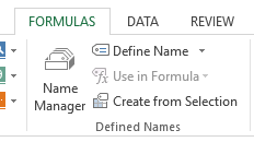
Click the Formulas tab and select the Name Manager option in the Defined Names group. This process opens the Name Manager tool.

Note: You can also open the Name Manager tool using the keyboard shortcut Ctrl + F3.

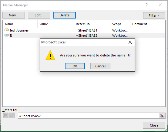
In the Name Manager window, select James_Washington_Math_Score in the list of defined names and click the Delete button. Please note that if you want to delete multiple names at once, you can select them by holding down the Ctrl key and clicking on them one after the other.

A message box appears asking you whether you are sure you want to delete the name James_Washington_Math_Score.

Prompt to confirm deleting the defined name

Click OK on the warning message box that appears.

The name is removed from the list of names in the Name Manager window.

Click the Close button to close the Name Manager.

If you check the Name box, you see that James_Washington_Math_Scores no longer appears.

Filtering for and Deleting Specific Defined Names

Sometimes, your workbook may have too many names to select individually.

That is where the filter option in the Name Manager comes in handy to filter for specific types of names before deleting them.

For instance, if you want to remove only the defined names scoped to the active worksheet, you do the following:

Press Ctrl + F3 to open the Name Manager.
Click the Filter button and select Names Scoped to Worksheet.

Only those names scoped to the worksheet will appear in the Name Manager window, making selecting and deleting them easy.

Deleting Names in a Protected Worksheet

Sometimes when you open the Name Manager tool, you may find that the Delete button is greyed out as follows:

This happens when the worksheet is protected. You cannot delete names in a protected worksheet.

You will need to unprotect the worksheet before deleting the names.

Click the Review tab and select Unprotect Sheet option in the Protect group. You may be required to supply the password used to protect the worksheet.

Method #2: Filter For Delete Defined Names Using Excel VBA

As helpful as the Filter option in the Name Manager tool is in filtering and deleting names, sometimes it can become tedious, especially when dealing with too many names. You can simplify the process by using the VBA code.

We use the following workbook with three defined names to show how we can use Excel VBA to filter for and delete specific names.

We want to filter for and delete only those defined names that contain the word Student.

We use the following steps:

Click the Developer tab and click Visual Basic in the Code group. This step opens the Visual Basic Editor.

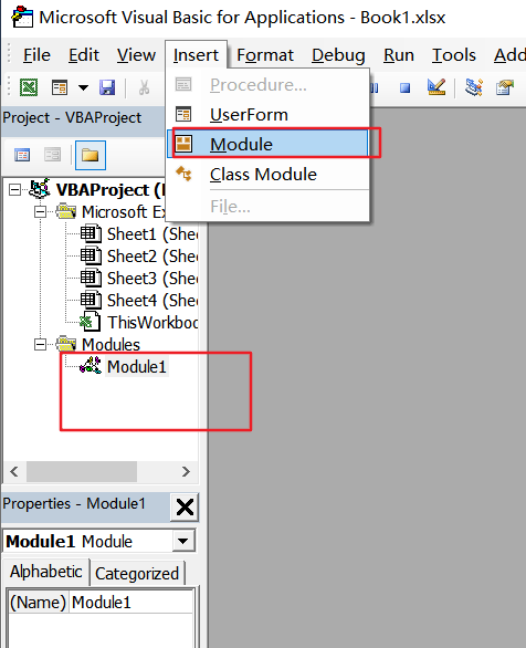
Click Module on the Insert Menu to create a new module in the Visual Basic Editor.

Type the following sub-procedure in the module:

'Code developed by Steve Scott from https://spreadsheetplanet.com
Sub FilterDeleteNames()
Dim FilteredName As Name
    For Each FilteredName In Application.ActiveWorkbook.Names
        If InStr(1, FilteredName.Name, "Student", vbTextCompare) > 0 Then FilteredName.Delete
    Next
End Sub

Save the sub-procedure and save the workbook as a Macro-Enabled Workbook.
Click inside the sub-procedure and press F5 to execute the code.
Click the View Microsoft Excel button on the toolbar to switch to the active workbook containing the dataset. You can also use the keyboard shortcut Alt + F11.
Open the Name Box and see that all the defined names that contain the word Student have been deleted.

Name Box and see that all the defined names

Method #3: Use Excel VBA to Delete All Defined Names

We may want to delete all defined names from a workbook at once. That‘s when Excel VBA comes in handy.

We will use the following worksheet with four defined names to show how we can use the Excel VBA to delete all defined names from a workbook.

We use the steps below:

Click the Developer tab and click Visual Basic in the Code group. The Visual Basic Editor is opened.

Note: You can also open the Visual Basic Editor using the keyboard shortcut Alt + F11.

Click Module on the Insert Menu to create a new module in the Visual Basic Editor.

Type the following sub-procedure in the module:

'Code developed by Steve Scott from https://spreadsheetplanet.com
Sub DeleteDefinedNames()
Dim dName As Name
    For Each dName In Application.ActiveWorkbook.Names
        dName.Delete
    Next
End Sub

Save the sub-procedure and save the workbook as a Macro-Enabled Workbook.
Click inside the procedure and press F5 to run the code.
Click the View Microsoft Excel button on the toolbar to switch to the active worksheet containing the dataset.

Open the Name Box and see that all the defined names have been deleted.

This tutorial has looked at three techniques for deleting defined names in Excel.

The methods include the application of the Name Manager tool, the Excel VBA to filter for and delete specific names, and Excel VBA to delete all the defined names in a workbook.

We hope that you found the tutorial helpful.

Other articles you may also like:

How to Rename a Table in Excel?
Excel Table vs. Excel Range – What’s the Difference?
How to Remove Table Formatting in Excel?

Источник

Delete one or more names

On the Formulas tab, in the Defined Names group, click Name Manager.
In the Name Manager dialog box, click the name that you want to change.
Select one or more names by doing one of the following: To select a name, click it.
Click Delete.
Click OK to confirm the deletion.

Contents

1 How do you delete a defined name range?
2 Why can’t I delete name in Excel?
3 How do I delete multiple names in Excel?
4 What is defined name in Excel?
5 How do you edit a defined table in Excel?
6 How do you delete a defined table in Excel?
7 How do I delete a named range in Excel without name manager?
8 How do I delete a hidden named range in Excel?
9 How do I mass delete words in Excel?
10 How do I mass delete data in Excel?
11 How do I delete multiple text boxes in Excel?
12 How do I remove first name and last name in Excel?
13 How do you edit a defined name in Excel?
14 How do you define names with values in Excel?
15 How do you edit a named range in Excel?
16 Where is named range in Excel?
17 How do you break name conflicts in Excel?
18 Why are there hidden names in Excel?
19 How do I delete just the text in Excel?
20 How do I delete all letters in Excel?

How do you delete a defined name range?

Alternatively, highlight the desired range, select the Formulas tab on the ribbon, then select Define Name. To manage range names, go to the Formulas tab, select Name Manager, choose a name, then select Delete or Edit.

Why can’t I delete name in Excel?

On Home ribbon select “Find & Select” Select Goto Special -> Validation and OK. All Data validation cells should be selected. Check the validation and use Clear all to delete the validation.

How do I delete multiple names in Excel?

Remove duplicate values

Select the range of cells that has duplicate values you want to remove. Tip: Remove any outlines or subtotals from your data before trying to remove duplicates.
Click Data > Remove Duplicates, and then Under Columns, check or uncheck the columns where you want to remove the duplicates.
Click OK.

What is defined name in Excel?

Excel name types
Defined name – a name that refers to a single cell, range of cells, constant value, or formula. For example, when you define a name for a range of cells, it’s called a named range, or defined range.

How do you edit a defined table in Excel?

Modifying tables

Select any cell in your table. The Design tab will appear on the Ribbon.
From the Design tab, click the Resize Table command. Resize Table command.
Directly on your spreadsheet, select the new range of cells you want your table to cover. You must select your original table cells as well.
Click OK.

How do you delete a defined table in Excel?

If your Excel worksheet has data in a table format and you no longer want the data and its formatting, here’s how you can remove the entire table. Select all the cells in the table, click Clear and pick Clear All. Tip: You can also select the table and press Delete.

How do I delete a named range in Excel without name manager?

Delete all named ranges with VBA code

Hold down the ALT + F11 keys, and it opens the Microsoft Visual Basic for Applications window.
Click Insert > Module, and paste the following code in the Module Window.
Then press F5 key to run this code, all names in the workbook will be removed immediately.

How do I delete a hidden named range in Excel?

But to get rid of this problem once and for all, here are few simple quick steps:

Delete all the visible name ranges. Do this by pressing Cntrl+F3.
Highlight all the name ranges you want to delete, and press delete.
Just a warning – a print area are also a “name range”.
Click “Delete”
Confirm by clicking “OK”

How do I mass delete words in Excel?

In the opening Find and Replace dialog, click the Replace tab, enter the specific word you will delete in the Find what box, keep the Replace with box empty, and then click the Replace All button. See screenshot: 3. Then a Microsoft Excel dialog pops out to tell you how many replacements it made.

How do I mass delete data in Excel?

1. Delete multiple rows in Microsoft Excel through the contextual menu

Open Microsoft Excel sheet which has the data you wish to manipulate.
From the data, select all the rows you want to delete in one stretch.
Now, right-click on the selection to open the contextual menu.
Hit ‘Delete’.

How do I delete multiple text boxes in Excel?

Just do the following steps:

#1 go to HOME tab, click Find & Select command under Editing group.
#2 Check Objects options in the Go To Special dialog box, click OK button.
#3 then you can press Delete key or Backspace key to delete all selected text boxes.

How do I remove first name and last name in Excel?

Read the steps

Add an empty column by right-clicking on the top of the column next to the existing column of names, then select Insert.
Click the Data tab.
Click on the top of the column with your contacts’ names to highlight the whole column.
Click Text to Columns.
Select “Delimited” and click Next.

How do you edit a defined name in Excel?

Edit a name

On the Formulas tab, in the Defined Names group, click Name Manager.
In the Name Manager dialog box, double-click the name you want to edit, or, click the name that you want to change, and then click Edit.
In the Edit Name dialog box, in the Name box, type the new name for the reference.

How do you define names with values in Excel?

Select Formulas > Create from Selection. In the Create Names from Selection dialog box, designate the location that contains the labels by selecting the Top row,Left column, Bottom row, or Right column check box. Select OK. Excel names the cells based on the labels in the range you designated.

How do you edit a named range in Excel?

Change a Named Range

On the Ribbon, click the Formulas tab.
Click Name Manager.
In the list, click on the name that you want to change.
In the Refers To box, change the range reference, or drag on the worksheet, to select the new range.
Click the check mark, to save the change.
Click Close, to close the Name Manager TOP.

Where is named range in Excel?

You can find a named range by using the Go To feature—which navigates to any named range throughout the entire workbook. You can find a named range by going to the Home tab, clicking Find & Select, and then Go To. Or, press Ctrl+G on your keyboard. In the Go to box, double-click the named range you want to find.

How do you break name conflicts in Excel?

Go to Formulas -> Name Manager, select the whole list in the pop up box and press Delete. Highly active question.

Why are there hidden names in Excel?

The Document Inspector found hidden names in your workbook. These names can store hidden information about Solver scenarios. For example, when you use the Solver add-in to run a scenario, it may store information about calculation parameters and other sensitive data as hidden names in your workbook.

How do I delete just the text in Excel?

1. Select the cells you need to remove texts and keep numbers only, then click Kutools > Text > Remove Characters. 2. In the Remove Characters dialog box, only check the Non-numeric box, and then click the OK button.

How do I delete all letters in Excel?

(1) You can type the formula =EXTRACTNUMBERS(A2,TRUE) into selected cell directly, and then drag the Fill handle to the range as you need. (2) This EXTRACTNUMBERS function will also remove all kinds of characters except the numeric characters.

Источник

Do you know what defined names are?

In Excel, you need to assign defined names to a cell or a range of cells, formulas, etc. Moreover, you can use them to produce maximum convenience when you need those factors to assign as data in similar or different sheets.

Here you will get to know how to delete defined names in Excel with the help of keyboard shortcuts, Formula tabs, and VBA macro coding. Let’s dive in to see how you can do this:

How to Delete Defined Names in Excel with Formula Tab

Open your workbook from which you need to delete the Defined Names.
Click on the Formulas Ribbon and then choose the Name Manager option.

You will see the Defined Names option given on the Name Manager screen.

Click on Defined Names to delete. In this example, we need to delete Allowance, Job_Id & Name. For this, you can press CTRL + Click on the Defined Names you need to delete.
Press the Delete button.

A warning window will pop up. Click OK.

Once again you will see the Name Manager window.

You will see other Defined Names.

How to Delete Defined Names in Excel with Keyboard Shortcuts

To open the Name Manager window, simply press CTRL + F3 keys from the keyboard. You will see the dataset has Defined Names including:

Press CTRL + F3 at once and the Name Manager Window will pop up.

Choose one or more Defined Names.
Press the Delete button.

You will see a warning dialog box. From this, click OK.

Here is the final result.

How to Delete Defined Names in Excel with VBA Macro

Here comes another complex but interesting method to delete defined names in Excel. For this, you can follow the steps given below:

You can see all the Defined Names are there in the dataset.

vba

Suppose you need to delete all of the existing Defined Names present in the dataset. For this, VBA Macro code is used.
Press SLT + F11 at once on your sheet. Microsoft Visual Basic window will pop up.
Open the Menu Bar and choose Module from the Insert menu.

vba2

Now, paste the following code into the Module.

vba3

Press F5 to run the code. Open the Excel sheet and check the Defined Name option given on the left side of the Formula Box.

You will notice all the Defined Names are deleted.

vba4

How Do You Edit Defined Names in Excel?

Do you know how would you edit defined names? With the help of Name Manager, you can simply edit the Defined Names. In case, you need to change the name or selected range, follow the steps given below:

Choose a cell from the dataset. Here we click on Cell B4.
Open the Formulas tab.
Click on the Name Manager option given in the Defined Names menu.

You will see the Name Manager window.

Here you will find all the Defined Names.
Choose the Name you need to edit.
Click on the Edit button.

The Edit Name window will pop up.

You will see the Name and referred cell references. Change the Name and press OK.

See the window appeared.

You will see the name of the selected Name edited and modified.

Summary

Defined Name in Excel is used for many reasons. However, sometimes you have to Delete Defined Names in Excel. You can use the above-mentioned methods without any fear of losing data. VBA Macro trick is awesome as it lets you execute a function just the way you want.

Источник

Delete a Defined Name & Named Range in Excel

Microsoft Excel is the powerful and advanced spreadsheet application which comes as part of Microsoft Office. EXcel allows users to define name for individual cell, cell range, function, constant or table in order to be used in formulas. The use of names in formulas make the formulas much easier to understand, track and maintain.

If you commonly create and add defined names, table names or named ranges in Excel, you may no longer need some of them. To keep the workbook and worksheets tidy, it’s a good practice to delete and remove unwanted or unused names using Excel’s Name Manager so that the workbook is clutter-free.

How to Delete a Defined Name or Named Range in Excel

Open the workbook that you want to clean up the defined names in Microsoft Excel.
On the Ribbon, go to Formulas tab, and tap or click on Name Manager in the Defined Names group.
Select the name or names (holding down Ctrl key to select multiple names, or Shift key to select a range of names contiguously) that you want to delete.
Click or tap on Delete button. Press OK again to confirm the deletion.

About the Author: LK

LK is a technology writer for Tech Journey with background of system and network administrator. He has be documenting his experiences in digital and technology world for over 15 years.Connect with LK through Tech Journey on Facebook, Twitter or Google+.

Page load link

Go to Top

Источник

In a Microsoft Excel worksheet, a cell can be given a name. And it is very EASY to name a cell: You click on the cell, put the cursor in the «Name Box» to the left of the Formula Bar, type a name, and press Enter. Then you can reference that cell by name in other parts of the workbook.

Also, when you click in a cell, if there is a cell name associated with that cell, it will display in the name box as shown in the worksheet image below.

In the example above we named the cell «Sub1» because we reference this Subtotal in a Summary worksheet.

However, after naming a cell, it seems like Excel won’t let you delete or change the name! Right? Because if you click in the Name Box and type over the name or delete the name, NOTHING HAPPENS! And Excel Help doesn’t seem to help.

So, how do I change or delete a cell name in an Excel spreadsheet? It’s pretty easy … it’s just hidden!

So open your Excel spreadsheet and follow the directions below.

1. Click the Formulas tab at the top of the worksheet. Then click Name Manager on the «Defined Names» section of the ribbon. The Name Manager window displays and lists ALL of the cell names that have ever been defined in the worksheets in that workbook.

2. Click on the cell name that you want to change, and click the Edit button. The Edit Name window displays.

3. Retype the name and click OK. When finished, click Close on the Name Manager window.

To Delete a Cell Name

2. Click on the cell name that you want to delete, and click Delete button.

3. Click OK on the «are you sure» popup and then click Close on the Name Manager window.

Whew! By the way, our main tutorial website has just had an exciting makeover! Besides our popular beginner’s tutorials such as Excel Math Basics: A Beginner’s Guide and Beginner’s Guide to Creating Charts in Excel, we’ve added tutorials on several more Excel functions, such as Nested IFs and Advanced Use of the COUNTIF Function.

Cheers!

Источник

Содержание

Use the Name Manager in Excel
Named Ranges in Excel: See All Defined Names (Incl. Hidden Names)
The problem of hidden defined names
The built-in Name Manager in Excel doesn’t show all defined names
Why not showing all names is a problem
Solution 1: Access named ranges manually
Solution 2: Use a VBA macro to see all named ranges
VBA macros to make all names visible
VBA macro to remove all names
Deleting All Names but a Few
How to Delete All Named Ranges in Excel
Method1: Delete All Named Ranges
Method2: Delete All Named Ranges with VBA

Use the Name Manager in Excel

Use the Name Manager dialog box to work with all the defined names and table names in a workbook. For example, you may want to find names with errors, confirm the value and reference of a name, view or edit descriptive comments, or determine the scope. You can also sort and filter the list of names, and easily add, change, or delete names from one location.

To open the Name Manager dialog box, on the Formulas tab, in the Defined Names group, click Name Manager.

The Name Manager dialog box displays the following information about each name in a list box:

One of the following:

A defined name, which is indicated by a defined name icon.

A table name, which is indicated by a table name icon.

Note: A table name is the name for an Excel table, which is a collection of data about a particular subject stored in records (rows) and fields (columns). Excel creates a default Excel table name of Table1, Table2, and so on, each time you insert an Excel table. You can change a table’s name to make it more meaningful. For more information about Excel tables, see Using structured references with Excel tables.

The current value of the name, such as the results of a formula, a string constant, a cell range, an error, an array of values, or a placeholder if the formula cannot be evaluated. The following are representative examples:

«this is my string constant»

The current reference for the name. The following are representative examples:

A worksheet name, if the scope is the local worksheet level.

«Workbook,» if the scope is the global workbook level. This is the default option.

Additional information about the name up to 255 characters. The following are representative examples:

This value will expire on May 2, 2007.

Don’t delete! Critical name!

Based on the ISO certification exam numbers.

The reference for the selected name.

You can quickly edit the range of a name by modifying the details in the Refers to box. After making the change you can click Commit to save changes, or click Cancel to discard your changes.

You cannot use the Name Manager dialog box while you are changing the contents of a cell.

The Name Manager dialog box does not display names defined in Visual Basic for Applications (VBA), or hidden names (the Visible property of the name is set to False).

On the Formulas tab, in the Defined Names group, click Define Name.

In the New Name dialog box, in the Name box, type the name you want to use for your reference.

Note: Names can be up to 255 characters in length.

The scope automatically defaults to Workbook. To change the name’s scope, in the Scope drop-down list box, select the name of a worksheet.

Optionally, in the Comment box, enter a descriptive comment up to 255 characters.

In the Refers to box, do one of the following:

Click Collapse Dialog (which temporarily shrinks the dialog box), select the cells on the worksheet, and then click Expand Dialog .

To enter a constant, type = (equal sign) and then type the constant value.

To enter a formula, type = and then type the formula.

Be careful about using absolute or relative references in your formula. If you create the reference by clicking on the cell you want to refer to, Excel will create an absolute reference, such as «Sheet1!$B$1». If you type a reference, such as «B1», it is a relative reference. If your active cell is A1 when you define the name, then the reference to «B1» really means «the cell in the next column». If you use the defined name in a formula in a cell, the reference will be to the cell in the next column relative to where you enter the formula. For example, if you enter the formula in C10, the reference would be D10, and not B1.

To finish and return to the worksheet, click OK.

Note: To make the New Name dialog box wider or longer, click and drag the grip handle at the bottom.

Источник

Named Ranges in Excel: See All Defined Names (Incl. Hidden Names)

Excel has a useful feature: Named Ranges. You can name single cells or ranges of cells in Excel. Instead of just using the cell link, e.g. =A1, you can refer to the cell (or range of cell) by using the name (e.g. =TaxRate). Excel also provides the “Name Manager” which gives you a list of defined names in your current workbook. The problem: It doesn’t show all names. Why that is a problem and how you can solve it is summarized in this article.

The built-in Name Manager in Excel doesn’t show all defined names

Please take a look at the screenshots below. On the left-hand side you can see the built-in Excel Name Manager (you can access it though Formulas–>Name Manager). The right-hand side is a screenshot of the Excel add-in “Professor Excel Tools” (more to that later). They were both taken with the same Excel workbook.

As you can see, the built-in Name Manager only shows none-hidden names. There are 4 names names in this workbook which are not hidden. But there are thousands more defined names in this particular workbook. Excel just doesn’t show them to you.

Why not showing all names is a problem

The problem with not showing all defined names is that you can’t delete them. Because they are hidden. Let’s talk a little bit about defined names in Excel.

Defined names are copied with each worksheet. So if your workbook has with thousands of names, they will be copied to a new workbook if you copy one worksheet.
Even if you delete the worksheet you copied, the defined names stay. That means, the name just keep accumulating.
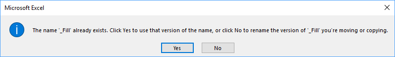
Besides that the names enlarge the workbook, you might run into trouble when duplicating worksheets. In worst case, you have to confirm the following dialogue box for each name separately.

Solution 1: Access named ranges manually

The first method is to access the source file of your Excel workbook. Please refer to this article for information about the source contents of an Excel file.

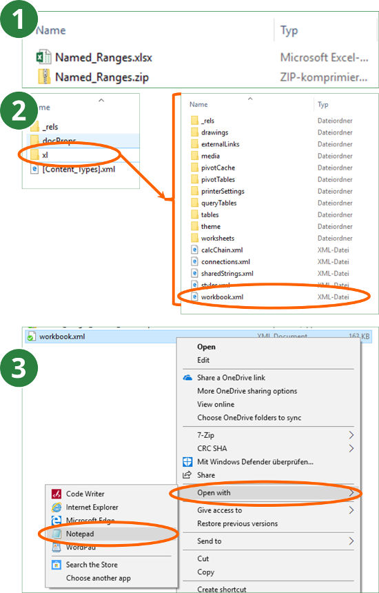
Create a copy of your Excel workbook and rename it. Delete .xlsx in the end and replace it with .zip.
Open the file and navigate to the folder “xl”. Copy the file “workbook.xml” and paste it into an empty folder outside the .zip-file.
Open the “workbook.xml” file with the text editor (right-click on the file and then on “Open with” –> “Notepad”). If you just want to see the named ranges without editing or removing them, you could also just double-click on the file “workbook.xml”. It usually opens in your web browser. The advantage: The layout is much better to read.
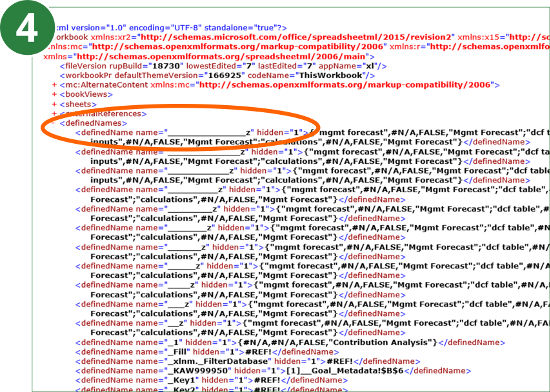
Now you can see all named ranges. They are listed between and .
Say, you want to remove all named ranges. Then you could delete all the content between and .
After editing the file you should save it and copy it back into the .zip-file. Replace the existing “workbook.xml” file there. Rename the complete .zip-file back to .xlsx. Now you can open it. Excel might notice that you changed the file and ask you if you’d like to recover as much as possible.

Please note: Tempering with the source code of your Excel file might damage the file. So please only work with copies of your file.

Solution 2: Use a VBA macro to see all named ranges

Our next method to edit hidden names in Excel is via VBA macros. We have prepared two VBA macros. Please insert a new VBA module and paste the following codes. If you need assistance concerning macros, please refer to this article.

VBA macros to make all names visible

This first VBA macros makes all defined names visible. You can then edit them within the built-in Name Manager (go to Formulas–>Name Manager). After pasting this code snipped into the new module, place the cursor within the code and click on the play button on the top of the VBA editor (or press F5 on the keyboard).

If you want to hide all names in your current workbook, replace tempName.Visible = True by tempName.Visible = False.

VBA macro to remove all names

The following VBA macros deletes all names in your workbook.

One word of caution: Print ranges and database ranges are also stored as defined names. Before you delete all names, make sure that you really don’t need them any longer.

Источник

Deleting All Names but a Few

Written by Allen Wyatt (last updated August 19, 2021)
This tip applies to Excel 97, 2000, 2002, and 2003

Do you routinely work with worksheets that contain dozens (or hundreds) of named cells, and most of those names are unnecessary? Cleaning up the names is a huge task, but getting rid of the ones you don’t need can make your workbook smaller and more efficient. The problem is, how do you get rid of a lot of unnecessary names all at once? You can certainly delete them one at a time, but such a process quickly gets tiresome.

One possible solution is to simply create a new workbook and copy the cells from the old workbook to the new one. Highlight the cells in the old workbook, use Ctrl+C to copy them, then paste them into worksheets in the new workbook. This will copy almost everything from the old workbook—formulas, formatting, etc. It does not bring copy over print settings or range names. The only task then remaining is to redefine the few names you want in the new workbook.

If you prefer to work with the old workbook (the one with all the names), it is best to create a macro that will do the name deletion for you. You need a macro that will allow you to delete all the names except those you want to keep. The following is a simple approach that accomplishes this task:

Before using the macro, modify the line that creates the vKeep array. Simply enter the names you want to keep within the array, each name surrounded by quotes and separated by commas. (In the example shown here, the names «Name1» and «Name2» will be kept.) The macro loops through all the names in the workbook and uses the Match function to see if the name is one in the array. If it is not, then it is deleted.

If you prefer to use a third-party solution to managing the names in your workbook, a great choice is the Name Manager add-in, written by Jan Karel Pieterse. You can find more information on the add-in here:

ExcelTips is your source for cost-effective Microsoft Excel training. This tip (2419) applies to Microsoft Excel 97, 2000, 2002, and 2003. You can find a version of this tip for the ribbon interface of Excel (Excel 2007 and later) here: Deleting All Names but a Few.

Author Bio

With more than 50 non-fiction books and numerous magazine articles to his credit, Allen Wyatt is an internationally recognized author. He is president of Sharon Parq Associates, a computer and publishing services company. Learn more about Allen.

Источник

How to Delete All Named Ranges in Excel

This post will guide you how to remove all named ranges from your workbook in Excel. How do I quickly delete all named ranges with VBA in Excel 2013/2016.

Method1: Delete All Named Ranges
Method2: Delete All Named Ranges with VBA

Assuming that you have created lots of named ranges in your workbook, and you wish to delete all of them at once, how to do it. You can use an Excel VBA macro to accomplish it. And this post will show you two methods to remove all named ranges.

Method1: Delete All Named Ranges

You can use Name Manager feature to delete all named ranges in your workbook, just see the following steps:

Step1: go to the Formulas tab, click Name Manager command under the Defined Names group. And the Name Manager dialog will open.

Step2: select the first name range in the Name Manager dialog box, and press Shift key to select the all the named ranges.

Step3: click Delete button at the top of the Name Manager dialog box, then a warning box will appear to ask you if you want to delete the selected names. Click Ok button. And all named ranges should be deleted at once.

Method2: Delete All Named Ranges with VBA

You can also use an Excel VBA Macro to remove all named ranges in a workbook. Just do the following steps:

Step1: open your excel workbook and then click on “Visual Basic” command under DEVELOPER Tab, or just press “ALT+F11” shortcut.

Step2: then the “Visual Basic Editor” window will appear.

Step3: click “Insert” ->”Module” to create a new module.

Step4: paste the below VBA code into the code window. Then clicking “Save” button.

Step5: back to the current worksheet, then run the above excel macro. Click Run button.

Источник

Как удалить имя в excel

В некоторых ситуациях удобнее пользоваться не адресами ячеек или диапазонами, а их именами. В частности, имена ячеек или диапазонов удобно использовать в формулах и при выполнении переходов. Присвоение имени может выполняться несколькими способами. Если предварительно был выделен блок, то независимо от выбранного способа имя будет присвоено соответствующему диапазону, если нет — текущей ячейке. Имя должно начинаться с буквы и не должно содержать пробелов.

Регистр букв значения не имеет. Все присвоенные имена доступны для использования во всех таблицах книги. Наиболее простой способ присвоения имя_ячейки имени:

1) установить табличный курсор на ячейку (выделить блок ячеек);

2) щелкнуть в секции адреса панели формул;

3) набрать имя и нажать Enter.

Ввод имени ячейки на панели формул

К такому же результату приведет следующая последовательность действий:

1) установить табличный курсор на ячейку (выделить блок ячеек);

2) вызвать окно Присвоение имени, для чего: — выполнить команду Имя-Присвоить. (Вставка) или — нажать CtrI+F3;

3) в поле ввода Имя набрать имя и нажать кнопку ОК.

Для завершения присвоения имени можно также нажать кнопку Добавить.

В этом случае окно Присвоение имени останется на экране. Для. отказа от присвоения имени можно нажать кнопку Закрыть. В поле Формула окна Присвоение имени появляется формула, в которой записан абсолютный адрес предварительно выделенной ячейки (диапазона ячеек) с указанием названия листа таблицы. При необходимости этот адрес можно заменить, причем удобнее это сделать, используя кнопку сворачивания окна. Понятно, что таким способом можно задать имя и без предварительного выделения ячейки (диапазона ячеек).

Если в создаваемой таблице заголовки строк и столбцов уже набраны, то для задания имен можно использовать еще один способ: 1) выделить блок ячеек, содержащий заголовки строк и (или) столбцов таблицы;

2) вызвать окно Создать имена, для чего: — выполнить команду Имя-Создать. (Вставка) или — нажать CtrI+Shift+F3;

3) выбрать один из переключателей и нажать кнопку ОК.

В этом случае имена будут присваиваться строкам и (или) столбцам выделенного блока. В качестве имени будет использоваться содержимое ячейки, указанной при выборе переключателя строки (столбца). Причем сама эта строка (столбец) в область, имеющую имя, включаться не будет.

В примере, будут созданы следующие пары (имя + диапазон): столбец_1 Лист1! $В$4:$В$6 столбец_2 Лист1! $С$4:$С$6 строка_1 Лист1!$В$4:$С$4 строка_2 Лист1!$В$5:$С$5 строка_3 Лист1! $В$6:$С$6

Во всех случаях создаваемому имени ставится в соответствие абсолютный адрес ячейки (ячеек), содержащий знак $. И именно этот адрес и будет подставляться в формулы вместо имен.

Для замены абсолютного адреса на относительный следует:

1) выполнить команду» Имя-Присвоитъ. (Вставка);

2) в открытом списке Имя диалогового окна Присвоение имени щелкнуть по имени ячейки (ячеек);

3) в поле Формула внести изменение, т. е. удалить знак $, и нажать кнопку ОК (для изменения можно выделить адрес и три раза нажать F4). Если для присвоения имени использовалось окно Присвоение имени, т. е. использовался второй способ, то такую замену адреса можно выполнить еще на этапе присвоения имени.

Имена можно присваивать не только ячейкам, но и формулам. Например, если формуле =$А$1+$В$1 присвоено имя Формула, то во всех случаях, когда необходимо вставить в ячейку эту формулу, можно набирать Формула. Для присвоения имени формуле необходимо:

1) выполнить команду Имя-Присвоить. (Вставка);

2) в поле Формула диалогового окна Присвоение имени набрать формулу;

3) в поле Имя ввести имя формулы и нажать кнопку ОК. Чтобы удалить имя, необходимо в открытом списке Имя окна Присвоение имени выделить имя и нажать кнопку Удалить.

Для быстрого перехода к ячейке (ячейкам), имеющей имя, можно открыть закрытый список в секции адреса панели формул и выбрать необходимое имя. Кроме этого, для перехода можно вызвать окно Переход, в поле Перейти к появившегося диалогового окна щелчком мыши выбрать имя (или набрать его в поле Ссылка) и нажать кнопку ОК.

Как удалить имя в excel

1) установить табличный курсор на ячейку (выделить блок ячеек);

2) щелкнуть в секции адреса панели формул;

3) набрать имя и нажать Enter.

Ввод имени ячейки на панели формул

К такому же результату приведет следующая последовательность действий:

1) установить табличный курсор на ячейку (выделить блок ячеек);

2) вызвать окно Присвоение имени, для чего: — выполнить команду Имя-Присвоить. (Вставка) или — нажать CtrI+F3;

3) в поле ввода Имя набрать имя и нажать кнопку ОК.

Для завершения присвоения имени можно также нажать кнопку Добавить.

2) вызвать окно Создать имена, для чего: — выполнить команду Имя-Создать. (Вставка) или — нажать CtrI+Shift+F3;

3) выбрать один из переключателей и нажать кнопку ОК.

Для замены абсолютного адреса на относительный следует:

1) выполнить команду» Имя-Присвоитъ. (Вставка);

2) в открытом списке Имя диалогового окна Присвоение имени щелкнуть по имени ячейки (ячеек);

1) выполнить команду Имя-Присвоить. (Вставка);

2) в поле Формула диалогового окна Присвоение имени набрать формулу;

Имена в EXCEL

Имя можно присвоить диапазону ячеек, формуле, константе или таблице. Использование имени позволяет упростить составление формул, снизить количество опечаток и неправильных ссылок, использовать трюки, которые затруднительно сделать другим образом.

Имена часто используются при создании, например, Динамических диапазонов , Связанных списков . Имя можно присвоить диапазону ячеек, формуле, константе и другим объектам EXCEL.

Ниже приведены примеры имен.

Объект именования

Пример

Формула без использования имени

Формула с использованием имени

имя ПродажиЗа1Квартал присвоено диапазону ячеек C20:C30

имя НДС присвоено константе 0,18

имя УровеньЗапасов присвоено формуле ВПР(A1;$B$1:$F$20;5;ЛОЖЬ)

имя МаксПродажи2006 присвоено таблице, которая создана через меню Вставка/ Таблицы/ Таблица

имя Диапазон1 присвоено диапазону чисел 1, 2, 3

А. СОЗДАНИЕ ИМЕН

Для создания имени сначала необходимо определим объект, которому будем его присваивать.

Присваивание имен диапазону ячеек

Создадим список, например, фамилий сотрудников, в диапазоне А2:А10 . В ячейку А1 введем заголовок списка – Сотрудники, в ячейки ниже – сами фамилии. Присвоить имя Сотрудники диапазону А2:А10 можно несколькими вариантами:

1.Создание имени диапазона через команду Создать из выделенного фрагмента :

выделить ячейки А1:А10 (список вместе с заголовком);
нажать кнопку Создать из выделенного фрагмента(из меню Формулы/ Определенные имена/ Создать из выделенного фрагмента );
убедиться, что стоит галочка в поле В строке выше ;
нажать ОК.

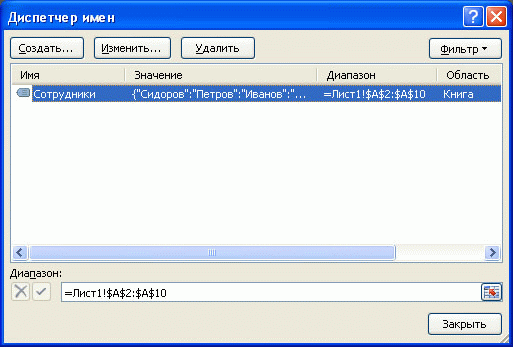
Проверить правильность имени можно через инструмент Диспетчер имен ( Формулы/ Определенные имена/ Диспетчер имен )

2.Создание имени диапазона через команду Присвоить имя :

выделитьячейки А2:А10 (список без заголовка);
нажать кнопку Присвоить имя( из меню Формулы/ Определенные имена/ Присвоить имя );
в поле Имя ввести Сотрудники ;
определить Область действия имени ;
нажать ОК.

3.Создание имени в поле Имя:

выделить ячейки А2:А10 (список без заголовка);
в поле Имя (это поле расположено слева от Строки формул ) ввести имя Сотрудники и нажать ENTER . Будет создано имя с областью действияКнига . Посмотреть присвоенное имя или подкорректировать его диапазон можно через Диспетчер имен .

4.Создание имени через контекстное меню:

выделить ячейки А2:А10 (список без заголовка);
в контекстном меню, вызываемом правой клавишей, найти пункт Имя диапазона и нажать левую клавишу мыши;
далее действовать, как описано в пункте 2.Создание имени диапазона через команду Присвоить имя .

ВНИМАНИЕ! По умолчанию при создании новых имен используются абсолютные ссылки на ячейки (абсолютная ссылка на ячейку имеет формат $A$1 ).

Про присваивание имен диапазону ячеек можно прочитать также в статье Именованный диапазон .

5. Быстрое создание нескольких имен

Пусть имеется таблица, в каждой строке которой содержится определенный массив значений.

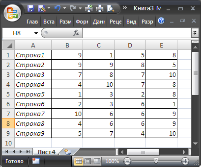
Необходимо создать 9 имен (Строка1, Строка2, . Строка9) ссылающихся на диапазоны В1:Е1 , В2:Е2 , . В9:Е9 . Создавать их по одному (см. пункты 1-4) можно, но долго.

Чтобы создать все имена сразу, нужно:

выделить выделите таблицу;
нажать кнопку Создать из выделенного фрагмента(из меню Формулы/ Определенные имена/ Создать из выделенного фрагмента );
убедиться, что стоит галочка в поле В столбце слева ;
нажать ОК.

Получим в Диспетчере имен ( Формулы/ Определенные имена/ Диспетчер имен ) сразу все 9 имен!

Присваивание имен формулам и константам

Присваивать имена формулам и константам имеет смысл, если формула достаточно сложная или часто употребляется. Например, при использовании сложных констант, таких как 2*Ln(ПИ), лучше присвоить имя выражению =2*LN(КОРЕНЬ(ПИ())) Присвоить имя формуле или константе можно, например, через команду Присвоить имя (через меню Формулы/ Определенные имена/ Присвоить имя ):

в поле Имя ввести, например 2LnPi ;
в поле Диапазон нужно ввести формулу =2*LN(КОРЕНЬ(ПИ())) .

Теперь введя в любой ячейке листа формулу = 2LnPi , получим значение 1,14473.

О присваивании имен формулам читайте подробнее в статье Именованная формула .

Присваивание имен таблицам

Особняком стоят имена таблиц. Имеются ввиду таблицы в формате EXCEL 2007 , которые созданы через меню Вставка/ Таблицы/ Таблица . При создании этих таблиц, EXCEL присваивает имена таблиц автоматически: Таблица1 , Таблица2 и т.д., но эти имена можно изменить (через Конструктор таблиц ), чтобы сделать их более выразительными.

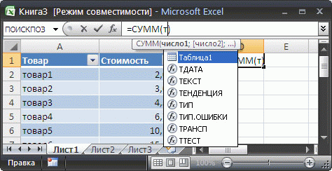
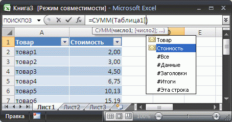
Имя таблицы невозможно удалить (например, через Диспетчер имен ). Пока существует таблица – будет определено и ее имя. Рассмотрим пример суммирования столбца таблицы через ее имя. Построим таблицу из 2-х столбцов: Товар и Стоимость . Где-нибудь в стороне от таблицы введем формулу =СУММ(Таблица1[стоимость]) . EXCEL после ввода =СУММ(Т предложит выбрать среди других формул и имя таблицы.

EXCEL после ввода =СУММ(Таблица1[ предложит выбрать поле таблицы. Выберем поле Стоимость .

В итоге получим сумму по столбцу Стоимость .

Ссылки вида Таблица1[стоимость] называются Структурированными ссылками .

В. СИНТАКСИЧЕСКИЕ ПРАВИЛА ДЛЯ ИМЕН

Ниже приведен список синтаксических правил, которым следует руководствоваться при создании и изменении имен.

Пробелы в имени не допускаются. В качестве разделителей слов используйте символ подчеркивания (_) или точку (.), например, «Налог_Продаж» или «Первый.Квартал».
Допустимые символы. Первым символом имени должна быть буква, знак подчеркивания (_) или обратная косая черта (). Остальные символы имени могут быть буквами, цифрами, точками и знаками подчеркивания.
Нельзя использовать буквы «C», «c», «R» и «r» в качестве определенного имени, так как эти буквы используются как сокращенное имя строки и столбца выбранной в данный момент ячейки при их вводе в поле Имя или Перейти .
Имена в виде ссылок на ячейки запрещены. Имена не могут быть такими же, как ссылки на ячейки, например, Z$100 или R1C1.
Длина имени. Имя может содержать до 255-ти символов.
Учет регистра. Имя может состоять из строчных и прописных букв. EXCEL не различает строчные и прописные буквы в именах. Например, если создать имя Продажи и затем попытаться создать имя ПРОДАЖИ , то EXCEL предложит выбрать другое имя (если Область действия имен одинакова).

В качестве имен не следует использовать следующие специальные имена:

Критерии – это имя создается автоматически Расширенным фильтром ( Данные/ Сортировка и фильтр/ Дополнительно );
Извлечь и База_данных – эти имена также создаются автоматически Расширенным фильтром ;
Заголовки_для_печати – это имя создается автоматически при определении сквозных строк для печати на каждом листе;
Область_печати – это имя создается автоматически при задании области печати.

Если Вы в качестве имени использовали, например, слово Критерии с областью действия Лист1, то оно будет удалено при задании критериев для Расширенного фильтра на этом листе (без оповещения).

С. ИСПОЛЬЗОВАНИЕ ИМЕН

Уже созданное имя можно ввести в ячейку (в формулу) следующим образом.

с помощью прямого ввода. Можно ввести имя, например, в качестве аргумента в формуле: =СУММ(продажи) или =НДС . Имя вводится без кавычек, иначе оно будет интерпретировано как текст. После ввода первой буквы имени EXCEL отображает выпадающий список формул вместе с ранее определенными названиями имен.
выбором из команды Использовать в формуле . Выберите определенное имя на вкладке Формула в группе Определенные имена из списка Использовать в формуле .

Для правил Условного форматирования и Проверки данных нельзя использовать ссылки на другие листы или книги (с версии MS EXCEL 2010 — можно). Использование имен помогает обойти это ограничение в MS EXCEL 2007 и более ранних версий. Если в Условном форматировании нужно сделать, например, ссылку на ячейку А1 другого листа, то нужно сначала определить имя для этой ячейки, а затем сослаться на это имя в правиле Условного форматирования . Как это сделать — читайте здесь: Условное форматирование и Проверка данных.

D. ПОИСК И ПРОВЕРКА ИМЕН ОПРЕДЕЛЕННЫХ В КНИГЕ

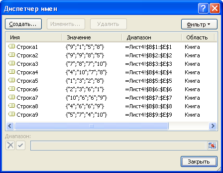
Диспетчер имен: Все имена можно видеть через Диспетчер имен ( Формулы/ Определенные имена/ Диспетчер имен ), где доступна сортировка имен, отображение комментария и значения.

Клавиша F3: Быстрый способ найти имена — выбрать команду Формулы/ Определенные имена/ Использовать формулы/ Вставить имена или нажать клавишу F3 . В диалоговом окне Вставка имени щелкните на кнопке Все имена и начиная с активной ячейки по строкам будут выведены все существующие имена в книге, причем в соседнем столбце появятся соответствующие диапазоны, на которые ссылаются имена. Получив список именованных диапазонов, можно создать гиперссылки для быстрого доступа к указанным диапазонам. Если список имен начался с A 1 , то в ячейке С1 напишем формулу:

Кликая по гиперссылке в ячейке С1 , будем переходить к соответствующим диапазонам.

Клавиша F5 (Переход): Удобным инструментом для перехода к именованным ячейкам или диапазонам является инструмент Переход . Он вызывается клавишей F5 и в поле Перейти к содержит имена ячеек, диапазонов и таблиц.

Е. ОБЛАСТЬ ДЕЙСТВИЯ ИМЕНИ

Все имена имеют область действия: это либо конкретный лист, либо вся книга. Область действия имени задается в диалоге Создание имени ( Формулы/ Определенные имена/ Присвоить имя ).

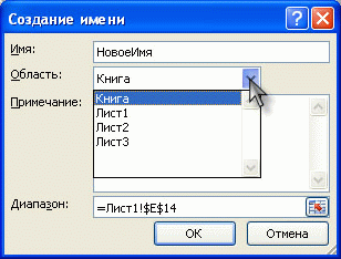
Например, если при создании имени для константы (пусть Имя будет const , а в поле Диапазон укажем =33) в поле Область выберем Лист1 , то в любой ячейке на Листе1 можно будет написать =const . После чего в ячейке будет выведено соответствующее значение (33). Если сделать тоже самое на Листе2, то получим #ИМЯ? Чтобы все же использовать это имя на другом листе, то его нужно уточнить, предварив именем листа: =Лист1!const . Если имеется определенное имя и его область действия Книга , то это имя распознается на всех листах этой книги. Можно создать несколько одинаковых имен, но области действия у них должны быть разными. Присвоим константе 44 имя const , а в поле Область укажем Книга . На листе1 ничего не изменится (область действия Лист1 перекрывает область действия Книга ), а на листе2 мы увидим 44.

Удалить имя диапазона в excel

Очередь просмотра

Очередь

Удалить все
Отключить

Хотите сохраните это видео?

Пожаловаться

Пожаловаться на видео?

Выполните вход, чтобы сообщить о неприемлемом контенте.

Понравилось?

Не понравилось?

Текст видео

Имя диапазона Excel используется для быстрого обращения к диапазону. После присвоения имени оно попадает в Диспетчер имён.
Записаться на консультацию: https://vk.com/id8547020

0:10 – присвоение имени столбцам таблицы в excel
0:50 – присвоение имени постоянный значениям в excel
1:47- автоматическое создание имен в excel из выделенного
2:43 – преобразование таблицы в именованный диапазон

[Alt]+[F3] – Переместить курсор в поле имя

[F3] – Вставить имя

[Ctrl]+[F3] – Открыть диспетчер имен

[Ctrl]+[Shift]+[F3] – Создать имя из выделенного диапазона
[Пробел] – Оператор для пересечения диапазонов

[F9] – Преобразовать ссылки в значения
[Ctrl]+[Shift]+[U] – Развернуть строку формул

Для чего вообще нужны именованные диапазоны? Обращение к именованному диапазону гораздо удобнее, чем прописывание адреса в формулах и VBA:

Предположим, что в формуле мы ссылаемся на диапазон A1:C10 (возможно даже не один раз). Для примера возьмем простую функцию СУММ(суммирует значения указанных ячеек):
=СУММ( A1:C10 ; F1:K10 )
Затем нам стало необходимо суммировать другие данные(скажем вместо диапазона A1:C10 в диапазоне D2:F11 ). В случае с обычным указанием диапазона нам придется искать все свои формулы и менять там адрес диапазона на новый. Но если назначить своему диапазону A1:C10 имя(к примеру ДиапазонСумм ), то в формуле ничего менять не придется – достаточно будет просто изменить ссылку на ячейки в самом имени один раз. Я привел пример с одной формулой – а что, если таких формул 10? 30?
Примерно такая же ситуация и с использованием в кодах: указав имя диапазона один раз не придется каждый раз при изменении и перемещении этого диапазона прописывать его заново в коде.
Именованный диапазон не просто так называется именованным. Если взять пример выше – то отображение в формуле названия ДиапазонСумм куда нагляднее, чем A1:C10 . В сложных формулах куда проще будет ориентироваться по именам, чем по адресам. Почему удобнее: если сменить стиль отображения ссылок (подробнее про стиль), то диапазон A1:C10 будет выглядеть как-то вроде этого: R1C1:R10C3 . А если назначить имя – то оно как было ДиапазонСумм , так им и останется.
При вводе формулы/функции в ячейку, можно не искать нужный диапазон, а начать вводить лишь первые буквы его имени и Excel предложит его ко вводу:

Данный метод доступен лишь в версиях Excel 2007 и выше

Как обратиться к именованному диапазону
Обращение к именованному диапазону из VBA

MsgBox Range(«ДиапазонСумм»).Address MsgBox [ДиапазонСумм].Address

Обращение к именованному диапазону в формулах/функциях

Если при указании диапазона в формуле выделить именованный диапазон, то его имя автоматически подставится в формулу вместо фактического адреса ячеек:

Ограничения, накладываемые на создание имен

В качестве имени диапазона не могут быть использованы словосочетания, содержащие пробел. Вместо него лучше использовать нижнее подчеркивание _ или точку: Name_1, Name.1
Первым символом имени должна быть буква, знак подчеркивания (_) или обратная косая черта (). Остальные символы имени могут быть буквами, цифрами, точками и знаками подчеркивания
Нельзя в качестве имени использовать зарезервированные в Excel константы – R, C и RC(как прописные, так и строчные). Связано с тем, что данные буквы используются самим Excel для адресации ячеек при использовании стиля ссылок R1C1 (читать подробнее про стили ссылок)
Нельзя давать именам названия, совпадающие с адресацией ячеек: B$100, D2(для стиля ссылок А1) или R1C1, R7(для стиля R1C1). И хотя при включенном стиле ссылок R1C1 допускается дать имени название вроде A1 или D130 – это не рекомендуется делать, т.к. если впоследствии стиль отображения ссылок для книги будет изменен – то Excel не примет такие имена и предложит их изменить. И придется изменять названия всех подобных имен. Если очень хочется – можно просто добавить нижнее подчеркивание к имени: _A1
Длина имени не может превышать 255 символов

Создание именованного диапазона
Способ первый
обычно при создании простого именованного диапазона я использую именно его. Выделяем ячейку или группу ячеек, имя которым хотим присвоить -щелкаем левой кнопкой мыши в окне адреса и вписываем имя, которое хотим присвоить. Жмем Enter:

Способ второй
Выделяем ячейку или группу ячеек. Жмем правую кнопку мыши для вызова контекстного меню ячеек. Выбираем пункт:

Excel 2007: Имя диапазона (Range Name)
Excel 2010: Присвоить имя (Define Name)

либо:
Жмем Ctrl + F3
либо:

2007-2016 Excel : вкладка Формулы (Formulas) –Диспетчер имен (Name Manager) –Создать (New) (либо на той же вкладке сразу – Присвоить имя (Define Name) )
2003 Excel : Вставка –Имя –Присвоить

Появляется окно создания имени

Имя (Name) – указывается имя диапазона. Необходимо учитывать ограничения для имен, которые я описывал в начале статьи.
Область (Scope) – указывается область действия создаваемого диапазона – Книга , либо Лист1 :

Лист1 (Sheet1) – созданный именованный диапазон будет доступен только из указанного листа. Это позволяет указать разные диапазоны для разных листов, но указав одно и тоже имя диапазона
Книга (Workbook) – созданный диапазон можно будет использовать из любого листа данной книги

Примечание (Comment) – здесь можно записать пометку о созданном диапазоне, например для каких целей планируется его использовать. Позже эту информацию можно будет увидеть из диспетчера имен ( Ctrl + F3 )
Диапазон (Refers to) – при данном способе создания в этом поле автоматически проставляется адрес выделенного ранее диапазона. Его можно при необходимости тут же изменить.

Изменение диапазона
Чтобы изменить имя Именованного диапазона, либо ссылку на него необходимо всего лишь вызывать диспетчер имен( Ctrl + F3 ), выбрать нужное имя и нажать кнопку Изменить (Edit. ) .
Изменить можно имя диапазона (Name) , ссылку (RefersTo) и Примечание (Comment) . Область действия (Scope) изменить нельзя, для этого придется удалить текущее имя и создать новое, с новой областью действия.

Удаление диапазона
Чтобы удалить Именованный диапазон необходимо вызывать диспетчер имен( Ctrl + F3 ), выбрать нужное имя и нажать кнопку Удалить (Delete. ) .

Так же можно создавать списки с автоматическим определением его размера. Например, если значения в списке периодически пополняются или удаляются и чтобы каждый раз не переопределять границы таких диапазонов. Такие диапазоны называют динамическими.

Статья помогла? Поделись ссылкой с друзьями!

В программе эксель для быстрого обращения к определенным ячейкам или прописыванию их в формуле, мы часто присваиваем имя ячейки, но иногда в ней необходимость отпадает и тогда возникает вопрос, как его удалить. Рассмотрим пошаговую инструкцию, как в программе эксель удалить имя ячейки.

Первый шаг. Перед нами лист, в котором есть таблица, а части ячейкам присвоено имена: «Массив» (присвоено диапазону ячеек) и «Элемент» (присвоено одной ячейки). Задача состоит в удаление имени «Элемент».

Второй шаг. Вам необходимо обратить внимание на верхнюю панель настроек, в которой нужно активировать закладку «Формулы», в неё есть блок «Определенные имена», в которой нам нужна иконка с надписью «Диспетчер имен».

Третий шаг. На экране появится дополнительное меню, в котором нужно найти название удаляемого имени, после его стоит выделить курсором и нажать на кнопку «Удалить». Как только вы закроете меню, имя названия данной ячейке исчезнет навсегда.

Источник