Skip to content
В этом руководстве вы узнаете, как можно легко удалить пустые столбцы в Excel с помощью макроса, формулы и даже простым нажатием кнопки.
Как бы банально это ни звучало, удаление пустых столбцов в Excel не может быть выполнено простым щелчком мыши. Это тоже нельзя сделать в два клика. Но всё же это можно сделать достаточно быстро и безошибочно. Перспективы просмотра всех колонок на листе и удаления незаполненных вручную – это определенно то, чего вам следует избегать. К счастью, Microsoft Excel предоставляет множество различных функций, и, используя их творчески, вы можете справиться практически с любой задачей!
Итак, как мы будем решать проблему удаления пустых столбцов?
- Способ 1 — быстрый, но неправильный.
- Способ 2 — макрос VBA.
- Способ 3 — используем формулы.
- Способ 4 — самый быстрый, одной кнопкой.
- Почему не удаляются пустые столбцы?
Быстрый, но неправильный способ удалить пустые столбцы.
Когда дело доходит до удаления пустот в таблице в Excel (будь то пустые ячейки, строки или столбцы), многие пользователи полагаются на команду Найти и выделить. Никогда не делайте этого на своих листах!
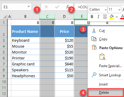
Этот метод ( Найти и выделить > Группу ячеек > Пустые ) находит и выбирает все пустые ячейки в диапазоне:
![]()
Если теперь щелкнуть выделенные ячейки правой кнопкой мыши и выбрать «Удалить» > « Весь столбец», то все колонки, содержащие хотя бы одну пустую ячейку, будут потеряны! Если вы сделали это случайно, нажмите Ctrl + Z , чтобы вернуть все на место.
Теперь, когда вы знаете неправильный способ удаления пустых столбцов в Excel, давайте посмотрим, как это сделать правильно.
Как удалить пустые столбцы в Excel с помощью VBA
Опытные пользователи Excel знают это практическое правило: чтобы не тратить часы на что-то вручную, потратьте несколько минут на написание макроса, который сделает это за вас автоматически.
Приведенный ниже макрос VBA удаляет все пустые столбцы в выбранном диапазоне. И делает это безопасно — удаляются только абсолютно пустые. Если столбец содержит значение хотя бы в одной ячейке, пусть даже пустую строку (“”), возвращаемую какой-либо формулой, то он останется на листе.
Public Sub DeleteEmptyColumns()
Dim SourceRange As Range
Dim EntireColumn As Range

On Error Resume Next
Set SourceRange = Application.InputBox( _
    "Select a range:", "Delete Empty Columns", _
    Application.Selection.Address, Type:=8)

If Not (SourceRange Is Nothing) Then
    Application.ScreenUpdating = False
    For i = SourceRange.Columns.Count To 1 Step -1
        Set EntireColumn = SourceRange.Cells(1, i).EntireColumn
        If Application.WorksheetFunction.CountA(EntireColumn) = 0 Then
            EntireColumn.Delete
        End If
    Next
    Application.ScreenUpdating = True
End If

End Sub
Вы можете в тексте макроса в шестой строке заменить сообщения на английском языке русскими. Однако, рекомендую оставить как есть во избежание проблем с отображением русских шрифтов в VBA.
Как использовать макрос удаления пустых столбцов
Вот пошаговая инструкция, чтобы добавить макрос в ваш файл Excel:
- Нажмите
Alt + F11, чтобы открыть редактор Visual Basic. - В строке меню щелкните Вставить > Модуль (Insert > Module).
- Вставьте приведенный выше код в появившееся окно. Нажмите иконку дискеты и сохраните проект.
- Если окно модуля еще открыто, то нажмите F5 для запуска макроса. В последующем для вызова программы используйте комбинацию Alt+F8.
- Когда появится всплывающее диалоговое окно, переключитесь на интересующий рабочий лист, выберите нужный диапазон и нажмите OK:
![]()
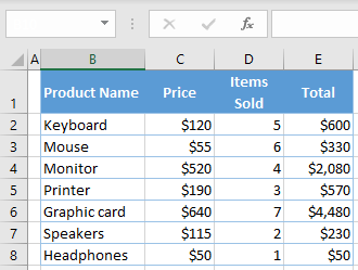
Пустые колонки в выбранном диапазоне будут удалены:
![]()
Однако, обратите внимание, что колонка, в которой есть название в шапке, но больше нет никакой информации, осталась нетронутой. Эту особенность нужно учитывать. Либо выбирайте при запуске макроса область, не включая в нее шапку таблицы.
Удаление пустых столбцов в Excel с помощью формул.
Вышеупомянутый макрос быстро и просто удаляет пустые столбцы. Но если вы относитесь к тому типу людей, которые «держит все под контролем» (как и я :), вы можете захотеть визуально увидеть те их них, которые будут удалены. В этом примере мы сначала определим пустые столбцы с помощью формулы, чтобы вы могли быстро их просмотреть, а затем удалим все или некоторые из них.
Примечание. Прежде чем удалять что-либо навсегда, особенно с помощью неопробованного вами метода, я настоятельно рекомендую вам сделать резервную копию своей книги, на всякий случай, если что-то пойдет не так.
Сохранив резервную копию в надежном месте, выполните следующие действия:
Шаг 1. Вставьте новую строку.
Добавьте новую строку вверху таблицы. Для этого щелкните правой кнопкой мыши заголовок первой строки и выберите Вставить. Не беспокойтесь о нарушении структуры таблицы и расположения ваших данных — вы сможете удалить её позже.
![]()
Шаг 2. Найдите пустые столбцы.
В самой левой ячейке только что добавленной строки введите следующую формулу:
=СЧЁТЗ(A2:A1048576)=0
Затем скопируйте формулу по строке на сколько это необходимо, перетащив маркер заполнения вправо.
Логика формулы очень проста: СЧЁТЗ проверяет количество пустых ячеек в столбце, от строки 2 до строки 1048576, что является максимумом числа строк в Excel 2019–2007. Вы сравниваете это число с нулем и в результате получаете ИСТИНА в пустых и ЛОЖЬ там, где имеется хотя бы одна непустая ячейка. Благодаря использованию относительных ссылок формула правильно настраивается для каждого столбца, в который она скопирована.
![]()
Если вы настраиваете лист для кого-то другого, вы можете пометить их более явным и понятным образом. Нет проблем, это легко сделать с помощью функции ЕСЛИ, примерно так:
=ЕСЛИ(СЧЁТЗ(A2:A1048576)=0;»Пусто»;»Не пусто»)
Теперь формула явным образом указывает, какие колонки пусты, а какие нет:
![]()
По сравнению с макросом этот метод дает больше гибкости в отношении того, какие колонки следует считать пустыми. В этом примере мы проверяем всю таблицу, включая строку заголовка. Это означает, что если столбец содержит только заголовок, то он не считается пустым и не удаляется. Если вы хотите проверять только строки данных, игнорируя заголовки, исключите строку (строки) заголовка из целевого диапазона. В результате он будет, к примеру, A3: A1048576. Имеющий заголовок, но не содержащий других данных, будет считаться пустым и посему подлежит удалению.
Кроме того, для быстроты расчетов вы можете ограничить диапазон до последней реально использованной в вашей таблице строки, которой в нашем случае будет A11.
Шаг 3. Удалите пустые столбцы.
Теперь вы можете просто выбрать те колонки, у которых в первой строке записано «Пусто» (чтобы выбрать сразу несколько, удерживайте Ctrl , нажимая на их буквы). Затем щелкните правой кнопкой мыши на любом из выделенных столбцов и укажите команду «Удалить» в контекстном меню:
![]()
Если на вашем листе десятки или сотни колонок, имеет смысл вывести на просмотр все пустые. Для этого сделайте следующее:
- Выберите верхнюю строку с формулами, перейдите на вкладку «Данные» > группу « Сортировка и фильтр » и нажмите кнопку «Сортировка» .
- В появившемся диалоговом окне с предупреждением выберите «Развернуть выделение» и нажмите «Сортировать…».
![]()
- Откроется диалоговое окно «Сортировка», в котором вы нажмете кнопку «Параметры…», выберите «столбцы диапазона» и нажмите «ОК» .
![]()
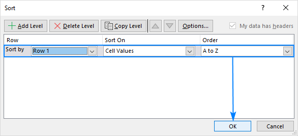
- Настройте только один уровень сортировки, как показано ниже, и нажмите ОК:
- Сортировать по: Строка 1
- Сортировка: значения ячеек
- Порядок: от А до Я
![]()
В результате пустые колонки будут перемещены в правую часть вашего рабочего листа, в конец таблицы:
![]()
Если вы выберете порядок сортировки от Я до А, то переместите их в левую чсть вашего листа, в начало.
- Выберите все пустые столбцы в конце таблицы. Для этого щелкните букву первого из них, нажмите Shift, а затем кликните на букву последнего.
- Щелкните правой кнопкой мыши на выделенном и выберите пункт «Удалить» во всплывающем меню.
Выполнено! Вы избавились от пустых столбцов, и теперь нет ничего, что могло бы помешать вам удалить верхнюю строку с формулами.
Самый быстрый способ удалить пустые столбцы в Excel.
В начале этого руководства я написал, что в Excel нет способа расправиться с пустыми столбцами одним щелчком мыши. На самом деле это не совсем так. Я должен был сказать, что нет таких стандартных возможностей в самом Excel. Пользователи надстройки Ultimate Suite могут удалить их почти автоматически, буквально за пару кликов 
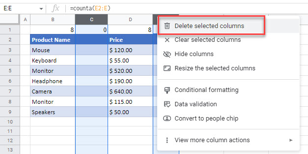
На вашем листе переключитесь на вкладку AblebitsTools, нажмите Delete Blanks и выберите Пустые столбцы (Empty Columns):
![]()
Чтобы убедиться, что это не случайный щелчок мыши, программа попросит вас подтвердить, что вы действительно хотите убрать пустые столбцы с этого рабочего листа:
![]()
Нажмите ОК, и через мгновение все незаполненные колонки исчезнут!
Как и описанный выше макрос, этот инструмент удаляет только те столбцы, которые абсолютно пусты. Колонки с одним значением, включая заголовки, сохраняются.
Более подробно об инструменте удаления пустых строк, столбцов и ячеек вы можете прочитать здесь.
Удаление пробелов – это лишь одна из десятков замечательных функций, которые могут облегчить вам жизнь пользователя Excel. Чтобы узнать больше, вы можете загрузить пробную версию невероятно функциональной программы Ultimate Suite for Excel.
Пустые столбцы не удаляются! Почему?
Проблема : вы испробовали все вышеперечисленные методы, но на вашем листе застряли одна или несколько пустых колонок. Почему?
Скорее всего, потому, что они на самом деле не пусты. Различные символы, невидимые глазу, могут незаметно скрываться в ваших таблицах Excel, особенно если вы импортировали информацию из внешнего источника. Это может быть просто пробел, неразрывный пробел или другой непечатаемый символ. Это также может быть формула, которая возвращает пустое значение.
Чтобы определить виновника, выберите первую ячейку в проблемном месте и нажмите Ctrl + стрелка вниз. И вы сразу же переместитесь к первой непустой ячейке. Например, столбец B на скриншоте ниже не является пустым из-за символа пробела в B6:
![]()
Дважды щелкните ячейку, чтобы перейти в режим редактирования и увидеть, что на самом деле находится в ней. Или просто нажмите клавишу Delete, чтобы избавиться от чего-то неизвестного и невидимого.
А затем повторите описанный выше процесс, чтобы узнать, есть ли ниже ещё какие-либо другие невидимые объекты. Вы также можете очистить свои данные, удалив начальные, конечные и неразрывные пробелы.
Благодарю вас за чтение и надеюсь увидеть вас в нашем блоге снова!
Deleting blank columns and rows is a tedious task when you are working with a large set of data. And manual deletion is not even an option. In this article, you’ll learn to delete the blank columns in excel in some simple steps using Excel built-in tool named Go To Special. It is a quick and easy way to remove the blank columns. While this makes it a simple alternative to implement, be aware that it may cause your document to become misaligned. Always save a backup copy of your document before you start deleting cells to be safe.
There are two ways to delete the blank columns in excel:
- Manual selection and deletion
- Deleting columns using Go To in-built tool from excel
Note: The tutorial is for Microsoft Excel 2013. You may find the same or different steps in other Microsoft Excel versions.
Deleting blank columns in Excel using manual selection and deletion
We can delete blank columns in Excel using manual selection and deletion. This method works with all types of data but it is time taking, here I would suggest to use this method only when your data is less. If you have a large number of columns to delete then move on to the second method. Now we understand this method with the help of an example. So consider the example

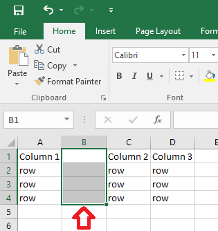
Step 1: Select the blank columns, to select the blank columns press Shift and press the down arrow to the row upto you want to select the column.

Step 2: Then right-click on the selected column. A drop-down will appear (as shown below). Select the Delete button. The selected column will be deleted.

Repeat the same steps for all the blank columns left in the required worksheet and delete them.
Deleting blank columns in Excel using Go To
We can also be deleting blank columns in MS Excel using Go To. So follow the following steps:
Step 1: Open the required Excel where you want to delete the blank columns.
Step 2: Select all the data by selecting the required rows and columns and press F5 from the keyboard. A dialogue box will appear(as shown below) and select Special. The special feature allows users to select all that has matching criteria as selected such as blanks, numbers, formulas.

Step 3: After selecting special, a window (as shown below) will appear. Click on Blanks (as shown) and then select OK. This operation will select all the blank columns from the selected data.

Step 4: Then go to the Home tab>Cells Group>Delete i.e go to the Home tab and in the Cells group click on Delete(as shown below). The delete will help to delete the selected row, column, cell, and entire sheet.

Step 5: After selecting Delete a drop-down will appear (as shown in the image). Select Delete Cells.

Step 6: After selecting Delete Cells, a pop-up window will appear(as shown below). Select Shift cells left. This option will shift all the leftover cells left after deleting the blank columns. Click OK.

All the blank columns from the selected range will be deleted.
Sometimes you may get an Excel dataset that has blank columns.
In most cases, this is undesirable and you would want to delete them. While there is no dedicated feature in Excel to delete blank columns in Excel, this is quite easy to do.
In this tutorial, I will show you four techniques for removing blank columns in Excel.
Note: We strongly recommend that you make a backup of your workbook before using any of the techniques so that in case anything goes wrong you have a backup of your data to revert to.
Method #1: Remove the Blank Columns Manually
In this method, we select each blank column and delete it manually.
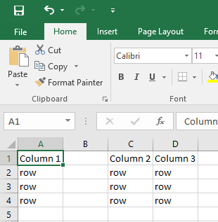
We use the following dataset which has two blank columns, columns C and G, to show how this technique works.

Below are the steps to delete blank columns manually:
- Select column C by clicking its column header, press and hold down the Ctrl key, select column G by clicking its column header, and then release the Ctrl key.

- Right-click inside any of the selected columns and choose Delete on the shortcut menu that appears.

The empty columns are removed from the dataset.

This technique is the best for small datasets but inefficient for large datasets that may have tens or even hundreds of blank columns.
Note: You can also select multiple columns in one go and then delete them together. To select multiple columns, hold the Control key and then select the columns you want to select by clicking the column headers
The following two methods come in handy when dealing with huge datasets.
Also read: Remove Blank Rows in Excel (5 Ways + VBA)
Method #2: Remove Blank Columns By Using a Formula With Find and Replace
In this technique, we first identify the empty columns using a formula and then delete them.
We will use the following example dataset that has columns C and G that appear blank to show how this technique can be used.

We say that columns C and G appear blank because we may not be too sure that the columns do not contain data in some cells that are way down the columns or even contain data in form of empty strings.
That is why we want to use a formula to first identify the empty columns before deleting them.
Below are the steps to identify all the columns that are empty:
- Insert a helper row on top of the dataset by right-clicking the header of row 1 and selecting Insert on the shortcut menu that appears.

- Enter the following formula in cell A1 of the helper row:
=IF(COUNTA(A2:A1048576)=0,"Blank","Not Blank")

- Press the Enter button on the Formula bar to enter the formula.
- Drag the fill handle across to column H to copy the formula to the columns.

The formula has returned the word Blank on top of all the empty columns. We can now remove the empty columns at once using the steps below:
- Select all the cells in the helper row.
- Press Ctrl + F to open the Find and Replace dialog box.
- In the Find and Replace dialog box that opens, do the following:
- Type the word Blank in the Find what drop-down.
- Open the Within drop-down and select Sheet.
- Open the Search drop-down and select By Rows.
- Select the Match entire cell contents option.
- Click the Find All button.

This returns the cell references of all the cells that contain the word Blank.
- Press Ctrl + A to select all the cells that contain the word Blank.

- Right-click any of the selected cells and select Delete on the shortcut menu that appears.

- In the Delete dialog box, select the Entire column option and then click OK.

All the blank columns are removed and data is shifted to the left.

You can now remove the helper row. We now have our dataset where the empty columns have been deleted.

Explanation of the formula
=IF(COUNTA(A2:A1048576)=0,"Blank","Not Blank")
This formula uses the COUNTA and IF functions.
The COUNTA function tallies the number of non-empty cells in a range.
The IF function checks whether a condition is met and returns TRUE if it is met and FALSE if it is not met.
- COUNTA(A2:A1048576)=0 In this part of the formula the COUNTA function returns TRUE if all the cells in the range A2: A1048576 are empty and returns FALSE if all the cells in the range are not empty. Note that the last row in all the new versions of Excel is row number 1,048,576.
- IF(COUNTA(A2:A1048576)=0, “Blank”, “Not Blank”) In this part of the formula the IF function returns Blank if the COUNTA function returns TRUE and returns Not Blank if the COUNTA function returns FALSE.
Note: If the columns only have column headers as in the example below, such columns are not considered blank. In such case, you need to modify the formula so it doesn’t include the headers

Method #3: Remove Blank Columns By Bringing Them Together Using the Sort Option
If our dataset has tens or even hundreds of non-contiguous blank columns, it is efficient to first bring them close to each other before deleting them.
Below I have a dataset where I want to remove all the empty columns.

First, I would use a formula to identify all the columns that are blank, and then I will use the Sort option to bring all the blank columns together so these can be removed in one go.
Below are the steps to identify all the columns that are empty:
- Insert a helper row on top of the dataset by right-clicking the header of row 1 and selecting Insert on the shortcut menu that appears.

- Enter the following formula in cell A1 of the helper row:
=IF(COUNTA(A2:A1048576)=0,"Blank","Not Blank")

- Copy the formula across column H to get the formula result on all the cells in the helper row.

The formula returns the word ‘Blank’ on top of all the empty columns, and the word ‘Not Blank’ in all the columns that are not blank.
Now that we know all the columns are empty, below are the steps to use the Sort option to bring all the empty columns together.
- Select the helper row which contains formulas by clicking its header.

- Click the Data tab, and select Sort in the Sort & Filter group.

- Select Expand the selection in the Sort Warning dialog box that opens up and click the Sort button.

- In the Sort dialog box, click the Options button.

- Select Sort left to right in the Sort Options dialog box that appears and then click on the OK button.

- In the Sort dialog box, open the Row Sort by drop-down and select Row 1, open the Sort On drop-down and select Cell Values, open the Order drop-down and select A to Z, and click OK:

All the blank columns are brought close to each other on the left of the worksheet as shown below:

- Select the first blank column by clicking its header, press and hold down the Shift key, select the last blank column by clicking its header, and then release the Shift key.

- Right-click the selected blank columns and select Delete on the shortcut menu that appears.

The blank columns are removed from the dataset:

We can now go ahead and remove the row we inserted on top of the dataset.
Your dataset is now free of blank columns.

Method #4: Remove Empty Columns Using VBA Macro Script
In this technique, we first create a subroutine in Excel VBA and then run the subroutine to remove the empty columns from the dataset.
We will use the below example dataset where columns C and G are blank and we need to remove these blank columns.

Follow the below steps to do this:
- Click the Developer tab and then click the Visual Basic icon in the Code group. This opens the Visual Basic Editor.

- Open the Insert menu and click the Module item. This inserts a new module in the Visual Basic Editor.

- Copy the following subroutine and paste it into the module.
'Code developed by Steve Scott from https://spreadsheetplanet.com
Sub RemoveBlankColumns()
Dim TargetRange As Range
Dim WholeColumn As Range
    Dim i As Long
    On Error Resume Next
    Set TargetRange = Application.InputBox( _
        "Select a range:", "Remove Blank Columns", _
        Application.Selection.Address, Type:=8)
If Not (TargetRange Is Nothing) Then
    Application.ScreenUpdating = False
    For i = TargetRange.Columns.Count To 1 Step -1
        Set WholeColumn = TargetRange.Cells(1, i).EntireColumn
            If Application.WorksheetFunction.CountA(WholeColumn) = 0 Then
                WholeColumn.Delete
            End If
    Next
Application.ScreenUpdating = True
End If
End Sub- Save the subprocedure and save the workbook as a Macro-Enabled workbook.
- Click inside the procedure and press F5 to run the code.
- When the InputBox pops up, switch to the worksheet containing the dataset you want to work with, select the dataset and click OK.

You will be taken back to the Visual Basic Editor.
- Click the View Microsoft Excel button on the toolbar to switch back to the active worksheet.

You will see that the empty columns have been removed from the dataset:

In this tutorial, we have looked at four techniques for removing blank columns in Excel. We can remove the blank columns manually, use a formula to identify the blank columns then delete them, and use Excel VBA. We hope you found this information beneficial.
Other articles you may also like:
- Fill Blank Cells with 0 in Excel
- How to Delete Hidden Rows or Columns in Excel?
- Fill Blank Cells with Dash (-) in Excel
- How to Fill Blank Cells with Value above in Excel
- How to Compare Two Columns in Excel (using VLOOKUP & IF)
- How to Remove Duplicate Rows based on one Column in Excel?
- How to Convert Columns to Rows in Excel?
Удаление пустых строк и столбцов в данных
Пустые строки и столбцы могут быть головной болью в таблицах во многих случаях. Стандартные функции сортировки, фильтрации, подведения итогов, создания сводных таблиц и т.д. воспринимают пустые строки и столбцы как разрыв таблицы, не подхватывая данные, расположенные за ними далее. Если таких разрывов много, то удалять их вручную может оказаться весьма затратно, а удалить сразу всех «оптом», используя фильтрацию не получится, т.к. фильтр тоже будет «спотыкаться» на разрывах.
Давайте рассмотрим несколько способов решения этой задачи.
Способ 1. Поиск пустых ячеек
Это, может, и не самый удобный, но точно самый простой способ вполне достойный упоминания.
Предположим, что мы имеем дело вот с такой таблицей, содержащей внутри множество пустых строк и столбцов (для наглядности выделены цветом):

Допустим, мы уверены, что в первом столбце нашей таблицы (колонка B) всегда обязательно присутствует название какого-либо города. Тогда пустые ячейки в этой колонке будут признаком ненужных пустых строк. Чтобы быстро их все удалить делаем следующее:
- Выделяем диапазон с городами (B2:B26)
- Нажимаем клавишу F5 и затем кнопку Выделить (Go to Special) или выбираем на вкладке Главная — Найти и выделить — Выделить группу ячеек (Home — Find&Select — Go to special).
- В открывшемся окне выбираем опцию Пустые ячейки (Blanks) и жмём ОК – должны выделиться все пустые ячейки в первом столбце нашей таблицы.
- Теперь выбираем на вкладке Главная команду Удалить — Удалить строки с листа (Delete — Delete rows) или жмём сочетание клавиш Ctrl+минус — и наша задача решена.
Само-собой, от пустых столбцов можно избавиться совершенно аналогично, взяв за основу шапку таблицы.
Способ 2. Поиск незаполненных строк
Как вы, возможно, уже сообразили, предыдущий способ сработает только в том случае, если в наших данных обязательно присутствую полностью заполненные строки и столбцы, за которые можно зацепиться при поиске пустых ячеек. Но что, если такой уверенности нет, и в данных могут содержаться и пустые ячейки в том числе?
Взгляните, например, на следующую таблицу — как раз такой случай:

Здесь подход будет чуть похитрее:
-
Введём в ячейку A2 функцию СЧЁТЗ (COUNTA), которая вычислит количество заполненных ячеек в строке правее и скопируем эту формулу вниз на всю таблицу:

- Выделим ячейку А2 и включим фильтр командой Данные — Фильтр (Data — Filter) или сочетанием клавиш Ctrl+Shift+L.
- Отфильтруем по вычисленному столбцу нули, т.е. все строки, где нет данных.
- Осталось выделить отфильтрованные строки и удалить их командой Главная — Удалить - Удалить строки с листа (Home — Delete — Delete rows) или сочетанием клавиш Ctrl+минус.
- Отключаем фильтр и получаем наши данные без пустых строк.

К сожалению, со столбцами такой трюк уже не проделать – фильтровать по столбцам Excel пока не научился.
Способ 3. Макрос удаления всех пустых строк и столбцов на листе
Для автоматизации подобной задачи можно использовать и простой макрос. Нажмите сочетание клавиш Alt+F11 или выберите на вкладке Разработчик — Visual Basic (Developer — Visual Basic Editor). Если вкладки Разработчик не видно, то можно включить ее через Файл — Параметры — Настройка ленты (File — Options — Customize Ribbon).
В открывшемся окне редактора Visual Basic выберите команду меню Insert — Module и в появившийся пустой модуль скопируйте и вставьте следующие строки:
Sub DeleteEmpty()
    Dim r As Long, rng As Range

    'удаляем пустые строки
    For r = 1 To ActiveSheet.UsedRange.Row - 1 + ActiveSheet.UsedRange.Rows.Count
        If Application.CountA(Rows(r)) = 0 Then
            If rng Is Nothing Then Set rng = Rows(r) Else Set rng = Union(rng, Rows(r))
        End If
    Next r
    If Not rng Is Nothing Then rng.Delete

    'удаляем пустые столбцы
    Set rng = Nothing
    For r = 1 To ActiveSheet.UsedRange.Column - 1 + ActiveSheet.UsedRange.Columns.Count
        If Application.CountA(Columns(r)) = 0 Then
            If rng Is Nothing Then Set rng = Columns(r) Else Set rng = Union(rng, Columns(r))
        End If
    Next r
    If Not rng Is Nothing Then rng.Delete

End Sub
Закройте редактор и вернитесь в Excel.
Теперь нажмите сочетание Alt+F8 или кнопку Макросы на вкладке Разработчик. В открывшемся окне будут перечислены все доступные вам в данный момент для запуска макросы, в том числе только что созданный макрос DeleteEmpty. Выберите его и нажмите кнопку Выполнить (Run) — все пустые строки и столбцы на листе будут мгновенно удалены.
Способ 4. Запрос Power Query
Ещё один способ решить нашу задачу и весьма частый сценарий — это удаление пустых строк и столбцов в Power Query.
Сначала давайте загрузим нашу таблицу в редактор запросов Power Query. Можно конвертировать её в динамическую «умную» сочетанием клавиш Ctrl+T или же просто выделить наш диапазон данных и дать ему имя (например Данные) в строке формул, преобразовав в именованный:

Теперь используем команду Данные — Получить данные — Из таблицы/диапазона (Data — Get Data — From table/range) и грузим всё в Power Query:

Дальше всё просто:
- Удаляем пустые строки командой Главная — Сократить строки — Удалить строки — Удалить пустые строки (Home — Remove Rows — Remove empty rows).
- Щёлкаем правой кнопкой мыши по заголовку первого столбца Город и выбираем в контекстном меню команду Отменить свёртывание других столбцов (Unpivot Other Columns). Наша таблица будет, как это технически правильно называется, нормализована — преобразована в три столбца: город, месяц и значение с пересечения города и месяца из исходной таблицы. Особенность этой операции в Power Query в том, что она пропускает в исходных данных пустые ячейки, что нам и требуется:
 таблицы")
- Теперь выполяем обратную операцию — сворачиваем полученную таблицу обратно в двумерную, чтобы вернуть ей исходный вид. Выделяем столбец с месяцами и на вкладке Преобразование выбираем команду Столбец сведения (Transform — Pivot Column). В открывшемся окне в качестве столбца значений выбираем последний (Значение), а в расширенных параметрах — операцию Не агрегировать (Don’t aggregate):

- Останется выгрузить результат обратно в Excel командой Главная — Закрыть и загрузить — Закрыть и загрузить в… (Home — Close&Load — Close&Load to…)

 таблицы")


Ссылки по теме
- Что такое макрос, как он работает, куда копировать текст макроса, как запустить макрос?
- Заполнение всех пустых ячеек в списке значениями вышестоящих ячеек
- Удаление всех пустых ячеек из заданного диапазона
- Удаление всех пустых строк на листе с помощью надстройки PLEX
Содержание
- Excel 2016 – How to delete all empty columns
- Tagged in
- One comment on “ Excel 2016 – How to delete all empty columns ”
- How to Delete Blank Columns in Excel?
- Deleting blank columns in Excel using manual selection and deletion
- Deleting blank columns in Excel using Go To
- How To Delete All Blank Columns in Microsoft Excel
- Using VBA Macro
- Using Excel Tools to Delete Blank Columns
- Deleting Blank Columns on Android
- Other Easy to Perform Sorting Tasks
- A Final Thought
- How to delete blank columns in Excel
- Quick way to delete empty columns that you should never use
- How to remove blank columns in Excel with VBA
- How to use the Delete Empty Columns macro
- Identify and delete blank columns in Excel with a formula
- Step 1. Insert a new row
- Step 2. Identify empty columns
- Step 3. Remove blank columns
- Fastest way to remove empty columns in Excel
- Blank columns are not deleted! Why?
Excel 2016 – How to delete all empty columns
The following steps show how to remove empty columns from an Excel spreadsheet using Excel 2016.
Note: this process does not account for partially empty columns. For example if a row in column 2 was empty that column would also be deleted.
![]()
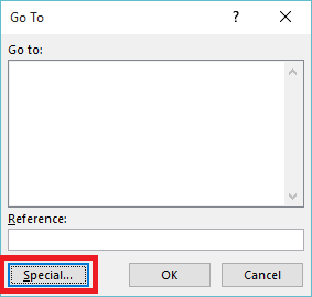
- With your spreadsheet open, press F5 on the keyboard. The ‘Go To’ window will open.
- Click on the ‘Special’ button

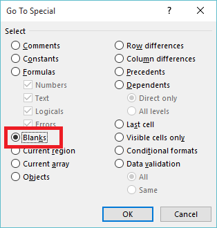
- Click on ‘Blanks’ then click ‘OK’
- This will select all the empty fields within your table.
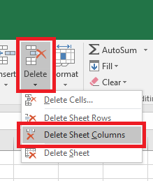
- In the ‘Home’ ribbon, click on the arrow below the ‘Delete’ button then click on ‘Delete Sheet Columns’
- Your empty columns have now been removed.
Tagged in
Hi
How to delete empty columns that are filled with color. For example, only empty columns that are blue should be removed, not empty red columns.
Источник
How to Delete Blank Columns in Excel?
Deleting blank columns and rows is a tedious task when you are working with a large set of data. And manual deletion is not even an option. In this article, you’ll learn to delete the blank columns in excel in some simple steps using Excel built-in tool named Go To Special. It is a quick and easy way to remove the blank columns. While this makes it a simple alternative to implement, be aware that it may cause your document to become misaligned. Always save a backup copy of your document before you start deleting cells to be safe.
There are two ways to delete the blank columns in excel:
- Manual selection and deletion
- Deleting columns using Go To in-built tool from excel
Note: The tutorial is for Microsoft Excel 2013. You may find the same or different steps in other Microsoft Excel versions.
Deleting blank columns in Excel using manual selection and deletion
We can delete blank columns in Excel using manual selection and deletion. This method works with all types of data but it is time taking, here I would suggest to use this method only when your data is less. If you have a large number of columns to delete then move on to the second method. Now we understand this method with the help of an example. So consider the example
Step 1: Select the blank columns, to select the blank columns press Shift and press the down arrow to the row upto you want to select the column.
Step 2: Then right-click on the selected column. A drop-down will appear (as shown below). Select the Delete button. The selected column will be deleted.
Repeat the same steps for all the blank columns left in the required worksheet and delete them.
Deleting blank columns in Excel using Go To
We can also be deleting blank columns in MS Excel using Go To. So follow the following steps:
Step 1: Open the required Excel where you want to delete the blank columns.
Step 2: Select all the data by selecting the required rows and columns and press F5 from the keyboard. A dialogue box will appear(as shown below) and select Special. The special feature allows users to select all that has matching criteria as selected such as blanks, numbers, formulas.
Step 3: After selecting special, a window (as shown below) will appear. Click on Blanks (as shown) and then select OK. This operation will select all the blank columns from the selected data.
Step 4: Then go to the Home tab>Cells Group>Delete i.e go to the Home tab and in the Cells group click on Delete(as shown below). The delete will help to delete the selected row, column, cell, and entire sheet.
Step 5: After selecting Delete a drop-down will appear (as shown in the image). Select Delete Cells.
Step 6: After selecting Delete Cells, a pop-up window will appear(as shown below). Select Shift cells left. This option will shift all the leftover cells left after deleting the blank columns. Click OK.
All the blank columns from the selected range will be deleted.
Источник
How To Delete All Blank Columns in Microsoft Excel
Every now and then, the data that you import from web pages may result in a great number of columns appearing even if they’re not used. You see this happening with CSV files and .txt files just as often.
![]()
When it happens, deleting columns manually may not always be easy. Sure, if you only have two or three empty columns, it’s quite ok to delete them manually. But what if your imported project creates 57 empty and non-continuous columns? – For that, you’ll need an automated process.
Using VBA Macro
The first method involves using a VBA macro.
- Go to your Excel file.
- Hold Alt + F11 together.
- Wait for the Microsoft Visual Basic for Applications window to appear.
- Then, click Insert.
- Select Module.
- Paste the following lines of code in the window.
Sub DeleteEmptyColumns()
‘Updateby20140317
Dim rng As Range
Dim InputRng As Range
xTitleId = «KutoolsforExcel»
Set InputRng = Application.Selection
Set InputRng = Application.InputBox(«Range :», xTitleId, InputRng.Address,Type:=8)
Application.ScreenUpdating = False
For i = InputRng.Columns.Count To 1 Step -1
Set rng = InputRng.Cells(1, i).EntireColumn
If Application.WorksheetFunction.CountA(rng) = 0 Then
rng.Delete
End If
Next
Application.ScreenUpdating = True
End Sub - Press F5 to compile and execute the macro.
- Input the appropriate work range in the dialog window.
The range is the specific interval between columns that you want to target. The format is $A$1:$J$12. The letters correspond to the column, and the numbers correspond to the rows. - Press OK.


After that, all the empty columns should be erased, and all filled columns should be next to each other.

Obviously, Excel wouldn’t be such a powerhouse if it didn’t have great sorting abilities. You can use the Delete dropdown menu to delete entire rows, columns, or blank cells.
- First, select the data range and press F5.
- Then, click Special.
- Now, select the Blanks option.
- Click OK (This selection will ensure that all blank cells are selected in the targeted range).
- Go to the Home tab.
- Select the Delete dropdown menu under the Cells tools group.
- Select Delete Cells.
- Select Shift cells left for removing and rearranging columns.
- Click OK.


Now the empty cells from the blank columns should’ve disappeared, and all the other rows are closer together.

You can use the same approach to delete entire rows. However, instead of moving the cells to the left, you select the other option.
Select Shift cells up for removing and rearranging rows.

Depending on what version of Excel you’re running, you may get different wordings. But in any case, the top two options in the Delete Cells menu are always the same.
This method no longer removes all blank cells in the selection. Before Excel 2013, this would inadvertently remove even empty rows, which would generally mess up the sorting.
Now the problem no longer occurs. Therefore, if you want to also get rid of the rows, you can do so by selecting the data range again and following the previous steps. Then simply select to shift or delete cells up instead of left.
Deleting Blank Columns on Android
Although the process is similar for deleting blank columns in Excel on Windows, Mac, and Android, here’s a quick overview of doing it on Android.
- Open up the Excel spreadsheet you want to edit and tap on the column heading you want to edit.
- Now, select Delete from the menu that appears.
Other Easy to Perform Sorting Tasks
Although using the Excel toolbar to delete empty columns and rows seems easier, the VBA macro method is foolproof, which means you can use it even in older Microsoft Excel versions.
Using the same VBA module or the Go To function menu, you can do so much more in Excel. Do you have certain formulas that are no longer relevant? – You can remove them as well or rearrange them accordingly.
You can also remove unnecessary comments or all comments from your project if you don’t want them to show up during your presentation. Look into VBA if you want to be an Excel power user.
A Final Thought
Over the years, a wide range of add-ons have appeared online. Some of them allow you to take even more shortcuts when sorting large spreadsheets. However, these apps are rarely free and not worth the trouble for simple tasks such as removing blank rows, cells, and columns.
Besides, if it were that difficult, Microsoft would’ve further simplified the process by now or created even more extensive guides on Excel sorting.
Источник
How to delete blank columns in Excel
 by Svetlana Cheusheva, updated on March 16, 2023
The tutorial will teach you how to remove empty columns in Excel with a macro, formula and a button-click.
As trivial as it sounds, deleting empty columns in Excel is not something that can be accomplished with a mere mouse click. It cannot be done in two clicks either. The prospect of reviewing all the columns in your worksheet and removing the empty ones manually is definitely something you’d want to avoid. Luckily, Microsoft Excel provides a great lot of different features, and by using those features in creative ways you can cope with almost any task!
Quick way to delete empty columns that you should never use
When it comes to removing blanks in Excel (whether it is empty cells, rows or columns), many online resources rely on the Go to Special > Blanks command. Never do that in your worksheets!
This method (F5 > Special… > Blanks) finds and selects all empty cells in the range: ![]()
If now you right-click the selected cells and choose Delete > Entire column, all the columns that contain at least one blank cell would be lost! If you’ve inadvertently did that, press Ctrl + Z to get everything back.
Now that you know a wrong way to delete blank columns in Excel, let’s see how to do it right.
How to remove blank columns in Excel with VBA
Experienced Excel users know this rule of a thumb: not to waste hours doing something manually, invest a few minutes in writing a macro that will do it for you automatically.
The below VBA macro removes all blank columns in the selected range. And it does this safely — only absolutely empty columns are deleted. If a column contains a single cell value, even an empty string returned by some formula, such a column will remain intact.
Excel macro: remove empty columns from Excel sheet
How to use the Delete Empty Columns macro
Here are the steps to add the macro to your Excel:
- Press Alt + F11 to open the Visual Basic Editor.
- On the menu bar, click Insert >Module.
- Paste the above code in the Code window.
- Press F5 to run the macro.
- When the pop-up dialog appears, switch to the worksheet of interest, select the desired range, and click OK:
![]()
If you do not want to add a macro to your worksheet, you can run it from our sample workbook. Here’s how:
- Download our sample workbook to Remove Blank Columns in Excel, open it, and enable content if prompted.
- Open your own workbook or switch to the already opened one.
- In your workbook, press Alt + F8 , select the DeleteEmptyColumns macro, and click Run.
- In the pop-up dialog, select the range and click OK.
![]()
Either way, all empty columns in the selected range will be disposed of: ![]()
Identify and delete blank columns in Excel with a formula
The above macro removes empty columns quickly and silently. But if you are a «keep-everything-under-control» kind of person (like I am 🙂 you may want to visually see the columns that are going to be removed. In this example, we will first identify blank columns by using a formula so that you could quickly review them, and then eliminate all or some of those columns.
Note. Before deleting anything permanently, especially by using an unknown technique, I strongly advise you to make a backup copy of your workbook, just to be on the safe side if something goes wrong.
With a backup copy in a safe place, perform the following steps:
Step 1. Insert a new row
Add a new row at the top of your table. For this, right-click the first row header and click Insert. Do not worry about mangling the structure/arrangement of your data — you can delete this row later. 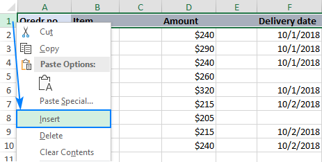
Step 2. Identify empty columns
In the leftmost cell of the newly added row, enter the following formula:
And then, copy the formula to the other columns by dragging the fill handle.
The formula’s logic is very simple: COUNTA checks the number of blanks cells in the column, from row 2 to row 1048576, which is a row maximum in Excel 2019 — 2007. You compare that number with zero and, as the result, have TRUE in blank columns and FALSE in the columns that contain at least one non-empty cell. Due to the use of relative cell references, the formula properly adjusts for each column where it is copied. ![]()
In case you are setting up the worksheet for someone else, you may want to label the columns in a more meaningful manner. No problem, this can be easily done with an IF statement similar to this:
=IF(COUNTA(A2:A1048576)=0, «Blank», «Not blank»)
Now the formula explicitly indicates which columns are empty and which are not: ![]()
Tip. Compared to a macro, this method gives you more flexibility with regard to which columns should be considered blank. In this example, we check the whole table, including the header row. That means if a column contains only a header, such a column is not regarded as blank and is not deleted. If you’d like to check only data rows ignoring column headers, remove the header row(s) from the target range (A3:A1048576). As the result, a column that has a header and no other data in it will be deemed blank and subject to deleting. Also, you can limit the range to the last used row, which would be A11 in our case.
Step 3. Remove blank columns
Having a reasonable number of columns, you can simply select those that have «Blank» in the first row (to select multiple columns, hold the Ctrl key as you click the column letters). Then, right-click any selected column, and choose Delete from the context menu: ![]()
If there are tens or hundreds of columns in your worksheet, it makes sense to bring all empty ones to view. For this, do the following:
- Select the top row with formulas, go to the Data tab >Sort and Filter group, and click the Sort button.
- In the warning dialog box that appears, select Expand the selection, and click Sort…
- This will open the Sort dialog box, where you click the Options… button, select Sort left to right, and click OK.
- Configure just one sort level like shown below and click OK:
- Sort by: Row 1
- Sort On: Cell Values
- Order: A to Z


As the result, the blank columns will be moved to the left part of your worksheet: ![]()
Done! You’ve got rid of the blank columns, and there is nothing that would now prevent you from deleting the top row with the formulas.
Fastest way to remove empty columns in Excel
In the beginning of this tutorial, I wrote that there is no one-click way to delete blank columns in Excel. In fact, that isn’t exactly true. I should have said there is no inbuilt way. The users of our Ultimate Suite can remove blanks in Excel literally in a couple of clicks 🙂
In the target worksheet, switch to the Ablebits Tools tab, click Delete Blanks and choose Empty Columns: ![]()
To make sure that wasn’t an accidental mouse click, the add-in will ask you to confirm that you really want to remove empty columns from that worksheet: ![]()
Click OK, and in a moment all blank columns are gone!
Like the macro discussed above, this tool deletes only those columns that are absolutely empty. Columns that have any single value, including headers, are preserved.
Delete Blanks is just one of tens of wonderful features that can make your life as an Excel user easier. To find more, you are welcome to download a trial version of our Ultimate Suite for Excel.
Blank columns are not deleted! Why?
Issue: You have tried all of the above methods, but one or more empty columns are stuck in your worksheet. Why?
Most likely because those columns are not really empty. Many different characters invisible to the human eye may lurk unnoticed in your Excel spreadsheets, especially if you imported information from an external source. That can be a mere empty string or a space character, non-breaking space or some other non-printing character.
To pin down the culprit, select the first cell in the problematic column and press Ctrl + down arrow . For example, column C in the screenshot below is not blank because of a single space character in C6: ![]()
Double-click the cell to see what actually is in it or simply press the Delete key to get rid of the unknown something. And then repeat the above process to find out if there are any other invisible things in that column. You may also want to clean your data by removing leading, trailing and non-breaking spaces.
I thank you for reading and hope to see you on our blog next week!
Источник
When I was working as a data analyst years ago, part of my job was to download data from financial databases and then clean this data.
And one of the things I had to do while cleaning the data was to delete any blank columns in the data set.
While you can always manually select columns and delete them one by one, doing so in a large data set, where you have tens or hundreds of columns in every data set, would be inefficient and error-prone.
While there is no inbuilt functionality in Excel to date blank columns in one go, this can be achieved by using a combination of different functionalities.
In this tutorial, I will show you how to delete empty columns in Excel using a couple of different methods (including a simple VBA code).
Manually Deleting Blank Columns (Best with Small Datasets)
If you have a small data set such as the one shown below, it’s possible to manually select the blank columns, and delete them.

Below are the steps to delete blank columns manually in the above data set:
- Select the blank column that you want to delete by clicking on the column header of that column

- Once the blank column is selected, right-click on the selection
- Click on the ‘Delete’ option

The above steps would instantly delete the selected blank column, and shift the remaining data set to the left.
Pro Tip: You can also select multiple blank columns in one go by holding the Control key on your keyboard (or the Command key if you’re using a Mac OS), and then manually clicking on the column headers of all the blank columns that you want to select. Once all the blank columns are selected, you can right-click and then click on the Delete option to delete all blank columns in one go
The biggest drawback of this method is that it is manual and inefficient (however, it could be a preferred method with small datasets).
In case you have a large data set with lots of blank columns, it’s better to use the methods covered next
Delete Blank Columns Using COUNT Function + Sort/Find and Replace
Excel has an inbuilt functionality that allows you to quickly select blank cells (using the Go-To special dialog box as we will see later in this tutorial), but there is no way to quickly select only those columns that are empty.
So we will have to use a workaround to first identify those columns that have only blank cells in them and then delete these blank columns.
Below I have a data set where I have the sales figures of different stores for different items. As you can see there are some columns that are completely empty in the below data set.
Now there are a couple of methods you can use to remove blank columns from the dataset. Let’s have a look at each of these methods in detail.
Using the COUNTA formula with FIND and Replace
With large datasets, a better way to delete all blank columns is by inserting a helper row at the top and using a COUNTA formula to identify all the columns that are empty.
Once you have done that, you can use this helper row to quickly select all the blank columns and delete them in one go.
Below I have a data set where I have some blank columns that I want to remove.
Here are the steps to do that using the COUNTA function with a helper row:
- Select the first row of your data set by clicking on the row header (it’s the row number in grey on the left)

- With the entire first row selected, right-click and then click on Insert. This will insert a new row above the first row of your data set

- Enter the below formula in the first cell of the helper row and copy it for all the cells in the helper row
=IF(COUNTA(A2:A1048576)=0,"Blank","Not Blank")

The above formula uses the COUNTA function and calculates the total number of cells that are not empty in the specified range.
This formula is going to return a value greater than zero for all the columns that are not completely empty and zero for any column that is completely empty.
And then I used the IF function to return “Blank” in a cell if the entire column below it is empty, and “Not Blank” if it is not empty.
Now that I can identify all the empty columns by looking at the values in the helper row, I’m going to use the Find and Replace dialog box to quickly select all the cells that have the value “Blank”.
Once I have these cells selected, I can delete the entire column in one go.
Below are the steps two now select all the empty columns in one go:
- Select all the cells in the helper row (the one where we entered the COUNTA formula)
- Hold the Control key on your keyboard and then press the F key. This will open the Find and Replace dialog box. You can also open the Find and Replace dialog box by going to the ‘Home’ tab and then clicking on the ‘Find & Select’ option and then clicking on the ‘Find’ option

- In the Find and Replace dialog box, enter the text ‘Blank’ in the ‘Find what’ field

- Click the ‘Options’ button

- In the ‘Look in’ drop-down, select ‘Values’
- Check the option, ‘Match entire cell contents’

- Click on the Find All button. This will find and return the cell references of all the cells that contain only the text ‘Blank’

- Hold the Control key and press the A key. This will select all the cells that were given by the Find and Replace option

- Right-click on any of the cells that have been selected (which would be any cell that has the text ‘Blank’ in it), and then click on ‘Delete’

- In the Delete dialog box, select the ‘Entire Column’ option

- Click OK
The above options would instantly delete all the blank columns in your data set.
Important Notes:
- COUNTA function would only return 0 if all the cells in the column are blank. in case there is a header in the column that has no values in it and needs to be removed, you need to adjust the formula so that the header row is not used. For example, you can use the formula =IF(COUNTA(A3:A1048576)=0,”Blank”,”Not Blank”) in case even blank columns have headers
- For this formula to work, the columns need to actually be blank. For example, if there are space characters in the cells in the blank column, while they might appear to be empty, the COUNTA function would not consider it as blank.
Using the COUNTA Formula with Sort Option
Let me show you another smart way you can use to quickly delete all the empty columns in Excel.
In this method, we will still be using the COUNTA function to get ‘Blank’ or ‘Not Blank’ in the helper row based on whether the column is empty or not.
But instead of using the Find and Replace dialog box, we will use the Sort option
Below I have the same data set and I want to remove the blank columns.
Below are the steps to insert a helper row to identify columns that are empty:
- Select the first row of your data set by clicking on the row header
- Right-click and then click on Insert. This will insert a new row above the first row of your data set
- Enter the below formula in the first cell of the helper row and copy it for all the cells in the helper row
=IF(COUNTA(A2:A1048576)=0,"Blank","Not Blank")
The above formula would return the text “Blank” in cells where the column below it is empty and “Not Blank” when the column below it is not empty.
Now I can sort the entire data set using the helper row so that I get all the blank columns together and all the non-blank columns together
Below are the steps to do this:
- Select the entire data set, including the helper row
- Click the Data tab

- In the Sort and Filter group, click on the Sort icon. This will open the Sort dialog box

- Click the Options button

- In the ‘Sort Options’ dialog box that opens up, click on the ‘Sort left to right’ option

- Click OK
- Click the ‘Sort by’ drop-down and then select the ‘Row 1’ option

- Keep the Sort Order A to Z (in case it’s not that already)

- Click Ok
The above steps would sort the data based on the helper row and bring all the blank columns together and non-blank columns together (as shown below).

Once you have all the blank columns together, you can select these in one go, and then delete them.
And once you have deleted the blank columns, you can remove the helper row as well.
Delete Blank Columns Using VBA
While the methods covered above work great, they do require a little bit of a setup using a helper row.
In case you are comfortable with VBA, you may find it a little easier to use as compared with the two helper row methods covered above.
Below is the VBA code that will do this for you:
'Code Developed by Sumit Bansal from https://TrumpExcel.com

Sub DeleteBlankColumns()

Dim EntireColumn As Range
On Error Resume Next

Application.ScreenUpdating = False

        For i = Selection.Columns.Count To 1 Step -1
            Set EntireColumn = Selection.Cells(1, i).EntireColumn
            If Application.WorksheetFunction.CountA(EntireColumn) = 0 Then
                EntireColumn.Delete
            End If
        Next

Application.ScreenUpdating = True

End Sub
The above VBA code uses a simple For-Next loop to go through each column in the selection, and check whether the COUNTA value for all the cells in that column is zero or not.
In case the COUNTA function value is 0, it means that the column is empty and the VBA macro code deletes that column.
And in case the value of the COUNTA function is more than 0, it means that the column is not empty and it is not removed.
How to Use the above VBA Macro Code?
Below are the steps to use the above VBA code to delete empty columns in Excel:
- Select the data set that has the blank columns that you want to remove
- Click the Developer tab in the ribbon.
- Click the Visual Basic icon. This will open the VB editor back end in Excel.
- Click the Insert option in the menu and then click on Module. This will insert a new module which would be visible in the Project Explorer pane. (In case you do not see the Project Explorer pane, click on the View option then click on Project Explorer)

- Copy and paste the above VBA macro code into the module code window

- To run the macro, place the cursor anywhere in the code and then click on the green play icon in the toolbar or use the F5 key on your keyboard
The above steps would instantly run the code which would remove all the empty columns from the selected data set.
Caution: The changes done by the VBA macro code in your worksheet cannot be undone. So it’s always a good idea to create a backup copy of your original data before using the VBA code to delete empty columns
Delete Blank Columns Using Go-To Special
One final method that I want to show you to delete empty columns in Excel is by using the Go To Special dialog box.
While this method is the fastest among all the methods covered in this tutorial so far, you need to be extremely cautious when using this method (especially if you’re working with large datasets).
This is because it can be error-prone and can lead to deleting columns that are not completely blank.
So while I’m covering this method in this tutorial, I would not recommend you use this method, instead use the other methods covered in this tutorial.
If you decide to use this method , you should be absolutely sure that your data set has no blank cells in the columns that are not completely blank
Let’s see how this method works.
Below I have a data set where I have some columns that are empty and I want to remove these columns.
Here are the steps to do this using go to special dialog box:
- Select the entire data set
- Press the F5 key on your keyboard. This will open the Go To dialog box. You can also get the same thing if you click on the Home tab and in the Editing group, click on the Find & Select option and then click on the Go To option

- In the Go-To dialog box that opens up, click on the Special button

- In the ‘Go To Special’ dialog box that opens up, click on the Blanks option

- Click OK. The above steps would select all the blank cells in your data set.

- Once you have these blank cells selected, right-click on any of these blank cells in the empty columns, and then click on the Delete option.
- This will open the Delete dialog box where you can choose the Entire column option and then click on OK
The above steps would delete all the columns where there are blank cells
The Drawback of this method?
One big drawback of this method is that in case you have a couple of blank cells in otherwise filled columns, these would also be selected and these non-blank columns would also be deleted.
Below is an example where I have a couple of blank cells in the Printer and Scanner columns, and these were also selected when I use the ‘Go To Special’ dialog box.

Now if I go ahead with the above ‘Go To Special’ method and delete the empty columns, even the Printer and the Scanner columns would be deleted, which is not what I want.
This is why it is best to avoid this method to delete empty columns as it could also end up deleting some columns just because they had a few blank cells in them.
So these are some of the methods you can use to delete blank columns in Excel.
If you have a small data set and you only have a couple of blank columns, it is better to delete them manually.
And in case you have a large data set, you can either use the VBA method (which is fast and efficient), or use the helper row along with the sort feature or the find and replace feature to quickly select blank columns and delete them.
Note: The methods I have covered in this tutorial can also be used to delete blank rows in Excel. You would have to adjust the methods and the VBA code accordingly
Other Excel tutorials you may also like:
- Delete Blank Rows in Excel (with and without VBA)
- Fill Down Blank Cells Until the Next Value in Excel (3 Easy Ways)
- Insert a Blank Row after Every Row in Excel (or Every Nth Row)
- How to Highlight Blank Cells in Excel (in less than 10 seconds)
- How to Replace Blank Cells with Zeros in Excel Pivot Tables
The following steps show how to remove empty columns from an Excel spreadsheet using Excel 2016.
Note: this process does not account for partially empty columns. For example if a row in column 2 was empty that column would also be deleted.
- With your spreadsheet open, press F5 on the keyboard. The ‘Go To’ window will open.
- Click on the ‘Special’ button

- Click on ‘Blanks’ then click ‘OK’

- This will select all the empty fields within your table.

- In the ‘Home’ ribbon, click on the arrow below the ‘Delete’ button then click on ‘Delete Sheet Columns’

- Your empty columns have now been removed.
See all How-To Articles
This tutorial demonstrates how to delete blank columns in Excel and Google Sheets.
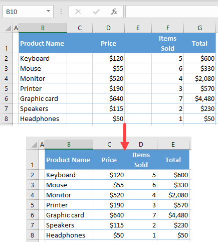
Delete Blank Columns
If you have a dataset containing blank columns, you can easily delete them using the COUNTA Function. Say you have the following dataset.
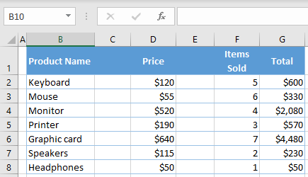
To delete empty columns completely, follow these steps:
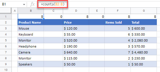
- Add one helper row above the dataset, and enter the formula in cell B1:
=COUNTA(B2:B1048576)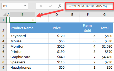
This formula counts all non-blank cells in the column.
- Now, copy the formula to the right, through to the last populated column (G).
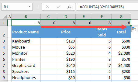
All blank columns have zeros in the first row.
- Select all columns with a value of 0 in the first row (C and E), right-click the selected area, and choose Delete.
- Now, all blank columns are deleted, and you can delete the helper row.
See also: How to Delete Blank Rows
Delete Blank Columns in Google Sheets
Following exactly the same steps, you can delete blank columns in Google Sheets.
The COUNTA formula is slightly different in Google Sheets; you do not need to add an end row to the formula.
=COUNTA(B2:B)
You can then select the columns that contain a zero and right-click on one of the selected column headers and select Delete selected columns.