Days and weeks excel

Let’s say you want to see the date displayed for a date value in a cell as «Monday» instead of the actual date of «October 3, 2005.» There are several ways to show dates as days of the week.

Note: The screenshot in this article was taken in Excel 2016. If you have a different version your view might be slightly different, but unless otherwise noted, the functionality is the same.

Format cells to show dates as the day of the week

1. Select the cells that contain dates that you want to show as the days of the week.

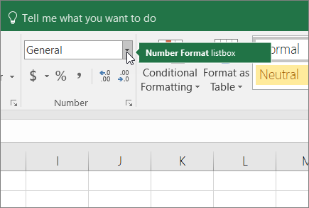
2. On the Home tab, click the dropdown in the Number Format list box, click More Number Formats, and then click the Number tab.

   

3. Under Category, click Custom, and in the Type box, type dddd for the full name of the day of the week (Monday, Tuesday, and so on), or ddd for the abbreviated name of the day of the week (Mon, Tue, Wed, and so on).

Convert dates to the text for the day of the week

To do this task, use the TEXT function.

Example

Copy the following data to a blank worksheet.

1 2 3

A Date 19-Feb-2007 3-Jan-2008 Formula Description (Result) =TEXT(A2, «dddd») Calculates the day of the week for the date and returns the full name of the day of the week (Monday) =TEXT(A3, «ddd») Calculates the day of the week for the date and returns the abbreviated name of the day of the week (Thu)

Need more help?

You can always ask an expert in the Excel Tech Community or get support in the Answers community.

See Also

TEXT

When working with date-specific information, there might be instances where you need to find the day of the week corresponding to a date.

For example, instead of the date, you may want to know whether it’s a Monday or a Tuesday or any other day.

This could be useful when working with to-do lists, daily/weekly summary reports, etc.

In this tutorial, we will see three different ways of converting dates to the corresponding day of the week in Excel.

For all the three methods in this tutorial, we will be using the following sample dataset.

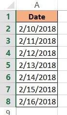
We will convert all the dates in the above sample dataset into corresponding days of the week.

Method 1: Converting Date to Day of Week in Excel using the TEXT Function

The TEXT function is a great function to convert dates to different text formats.

It takes a date serial number or date and lets you extract parts of the date to fit your required format.

Here’s the syntax for the TEXT function:

= TEXT (date, date_format_code)

In this function,

• date is the date, date serial number, or reference to the cell that you want to convert.
• date_format_code is the format code based on how you want the converted date to look.

The TEXT function applies the date_format_code that you specified on the provided date and returns a text string with that format.

For example, if you have the date “2/10/2018” in cell A2, then =TEXT(A2,”dddd”) will return “Saturday”.

Here, “dddd” is the date_format code to display the day of the week corresponding to date in full words.

Here are some basic building blocks for the format codes that you can use:

Format Codes for Day of the Week or Month:

You can use the following basic format codes to represent day values:

• d – one or two-digit representation of the day (eg: 3 or 30)
• dd – two-digit representation of the day (eg: 03 or 30)
• ddd – the day of the week in abbreviated form (eg: Sun, Mon)
• dddd – full name of the day of the week (eg: Sunday, Monday)

So,

• if you apply =TEXT(A2, “d”) to the sample dataset, it will return “10”.
• if you apply =TEXT(A2, “dd”), then it will return “10”.
• if you apply =TEXT(A2, “ddd”) to the sample dataset, it will return “Sat”.
• if you apply =TEXT(A2, “dddd”), then it will return “Saturday”.

Let us see how we can apply the TEXT function to our sample dataset to convert all the dates to days of the week.

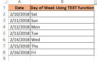
We will first see how to convert the dates in column A to the format shown in column B in the image below:

Below are the steps to convert the date to a weekday name using the TEXT function:

1. Click on a blank cell where you want the day of the week to be displayed (B2)
2. Type the formula: =TEXT(A2,”ddd”) if you want the shortened version of the day or =TEXT(A2,”dddd”) if you want the full version of the day.
3. Press the Return key.
4. This should display the day of the week in our required format. Copy this to the rest of the cells in the column by dragging down the fill handle or double-clicking on it.
5. Copy this column’s formula results by pressing CTRL+C or Cmd+C (if you’re on a Mac).
6. Right-click on the column, and from the popup menu that appears, press Paste Values from the Paste Options.
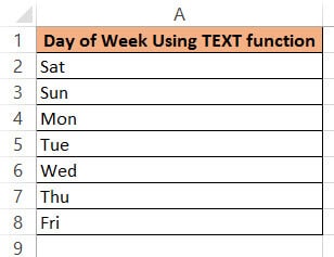
7. This will store the formula results as permanent values in the same column. Now you can go ahead and remove column A if you want to.

You should see all the dates converted to the short form of their corresponding days of the week:

The result you get in column B will differ according to the format code you used in step 2. Here are some format codes along with the type of result you will get when applied to cell A2:

Function	Result
=TEXT(A2, “ddd”)	Sat
=TEXT(A2, “dddd”)	Saturday

Note: Using this formula, your converted date is in text format, so you will see the results aligned to the left side of the cells.

Also read: How to Convert Date to Serial Number in Excel?

Method 2: Converting Date to Day of Week in Excel using the Format Cells Feature

The Format Cells feature provides a great way to directly convert your dates to days of the week while replacing the existing dates. As such you don’t need to have a separate column to type the formula.

You can use the Format Cells dialog box to convert your dates to days of the week as follows:

1. Select all the cells containing the dates that you want to convert (A2:A8).
2. Right-click on your selection and select Format Cells from the popup menu that appears. Alternatively, you can select the dialog box launcher in the Number group under the Home tab.
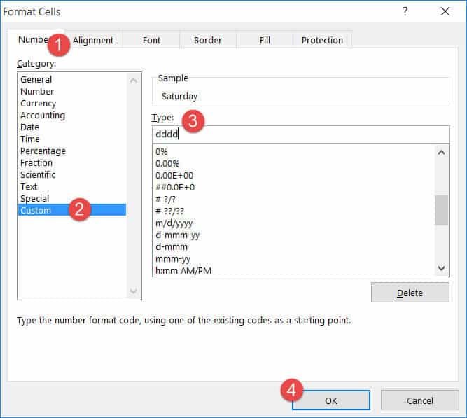
3. This will open the Format Cells dialog box. Click on the Number tab
4. Under Category on the left side of the box, select the Custom option.
5. This will display a number of formatting options on the right side, under Type. You can type in your format code in the Type field. You can type in “ddd” if you want the short form or “dddd” if you want the full form of the day.
6. Click OK to close the Format Cells dialog box.

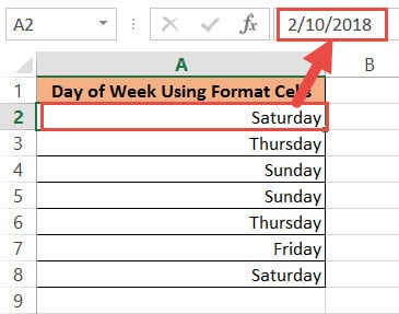
All your selected cells should now appear as weekday names.

Note: By using Format Cells, you have just changed the format in which the dates are displayed in the cells. The actual dates are underlying the cells and can be seen in the formula bar when a cell is selected.

Also read: How to Convert Text to Date in Excel?

Method 3: Converting Date to Day of Week in Excel using a Formula

If you’d rather use your own representation for the days of the week, you can use a formula based on both the WEEKDAY and CHOOSE functions.

First, let us understand these two functions individually.

The WEEKDAY Function

The WEEKDAY function converts a date to a number between 1 and 7, one for each day of the week. It chooses the sequencing of these numbers based on the day we want the week to begin from.

This is helpful because in some countries, the week starts from Sunday, while in others, especially Middle Eastern countries, the week starts from Saturday.

The syntax for the WEEKDAY function is:

WEEKDAY(date, [type])

Here,

• date is the input date for the function. It can be a date, a date serial number, or a reference to a cell that holds a date value.
• type is an optional parameter. It tells the function where to begin the week from. So, if we put a 1, it means the week should start from Sunday and end on Saturday. If we put a 2, it means the week should start from Monday and end on Sunday, and so on. By default, the value for the type parameter is set to 1.

In our example, WEEKDAY(A2, 1) will return 7, corresponding to a Saturday.

The CHOOSE Function

The CHOOSE function lets you specify a particular outcome depending on a value. For example, you can choose to display the word “red” if a value is 1, “blue” if it is 2, “green” if it is 3, and so on.

In this way it’s a great alternative to using a bunch of nested IF functions.

The syntax for the CHOOSE function is:

=CHOOSE (index, value1, [value2], ...)

Here,

• index is the input value. It can be any number between 1 and 254.
• value1 is the first value from the list of possible outputs
• value2 is the second value from the list of possible outputs,

etc.

The function returns value1 if index is 1, value2 if index is 2, etc.

So the function: =CHOOSE(3, “sun”,”mon”,”tue”,”wed”,”thu”,”fri”, ”sat”) will return “tue”, because it’s the third value in the list.

Putting the Formula Together

Let us put the two functions CHOOSE and WEEKDAY together to convert date to day of the week. Here are the steps to follow:

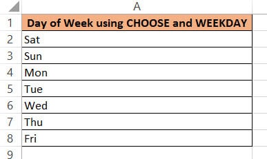
1. Click on a blank cell where you want the day of the week to be displayed (B2)
2. Type the formula: =CHOOSE(WEEKDAY(A2),”Sun”,”Mon”,”Tue”,”Wed”,”Thu”,”Fri”,”Sat”)
3. Press the Return key.
4. This should display the day of the week in short form, corresponding to the date in A2. Copy this to the rest of the cells in the column by dragging down the fill handle or double-clicking on it.
5. Copy this column’s formula results by pressing CTRL+C or Cmd+C (if you’re on a Mac).
6. Right-click on the column and form the popup menu that appears, press Paste Values from the Paste Options.
7. This will store the formula results as permanent values in the same column. Now you can go ahead and remove column A if you want to.

Here’s what you should get as the result:

How did this Formula Work?

To understand how this formula worked, we need to break it down:

1. First, we used the WEEKDAY function to find the number corresponding to the day of the week, assuming our week starts from Sunday. This will return a number between 1 and 7.
2. We used the output of the WEEKDAY function to find the string from the list of days [“sun”,”mon”,”tue”,”wed”,”thu”,”fri”, “sat”] corresponding to that number. So if the output for WEEKDAY(A2) was 7, then the corresponding output for the CHOOSE function will be the seventh item in the list, which is “sat”.

Thus we get the day corresponding to the date in A2 (in our example) to be “sat”.

Note: The above formula will give your converted date in text format, so you will see the results aligned to the left side of the cells.

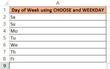
You could also have any other format for the days in the list, for example, if you wanted to display just the first two letters for the days, you could have written the formula in step 2 as:

=CHOOSE(WEEKDAY(A2),"Su","Mo","Tu","We","Th","Fr","Sa")

So you could get an output as:

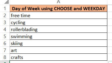
If you wanted to make a to-do list, you could even have an activity for each day of the week. For example, you could use the formula:

=CHOOSE(WEEKDAY(A2),"cycling","rollerblading","swimming","skiing","art","crafts","free time")

So you could get an output as:

In this tutorial, we saw three ways to convert a date to the day of the week.

The first method involves a function (TEXT), the second method involves a commonly used Excel dialog box (Format Cells) and the third method involves an Excel formula (with WEEKDAY and CHOOSE functions).

We hope you found this tutorial helpful and easy to apply to your data.

Other Excel tutorials you may find useful:

• How to Convert Serial Numbers to Date in Excel
• How to Convert Date to Month and Year in Excel
• How to Get Total Days in Month in Excel?
• How to Add Days to a Date in Excel
• How to Sort by Date in Excel (Single Column & Multiple Columns)
• Why are Dates Shown as Hashtags in Excel?
• How to Convert Month Number to Month Name in Excel
• How to Convert Days to Years in Excel (Simple Formulas)
• How to Get the First Day Of The Month In Excel?

What day of the week is 2019-11-14? Is it a Monday, Tuesday, Wednesday, etc…

It’s pretty common to want to know what day of the week a given date falls on and unless you’ve got some sort of gift for knowing that, you’re going to need a way to figure it out.

In Excel, there are many different ways to determine this. In this post, we’re going to explore 7 ways to achieve this task.

Format a Date as the Weekday Name

The first option we’re going to look at involves formatting our date cells.

Dates in Excel are really just serial numbers starting at 1 for the date 1900-01-01. Formatting is what makes the date look like a date.

There are many ways to format these serial numbers to display the date in various formats like yyyy-mm-dd, dd/mm/yyyy, dd-mmm-yy etc…

One of the possible formatting options for these serial numbers is to display the weekday name with a custom dddd or ddd format.

We can format our dates from the Format Cells dialog box.

1. Select the dates which we want to convert into weekday names.
2. Go to the Home tab and click on the small launch icon in the lower right corner of the Number section. This will open up the Format Cells dialog box. We can also open up the Format Cells dialog a few other ways.
   • The keyboard shortcut Ctrl + 1.
   • Right click on the selected cells ➜ choose Format Cells from the menu.
3. Go to the Number tab in the Format Cells dialog box.
4. Select Custom as the Category.
5. Add dddd into the Type field for the full weekday name or ddd for the abbreviated weekday name.
6. Press the OK button.

Now our dates will appear as the weekday names in the worksheet. The dates are still inside the cells and can be seen in the formula bar when a cell is selected.

Get the Weekday Name with the TEXT Function

The TEXT function will allow us to convert numbers to text and apply formatting to those numbers.

= TEXT ( 1234 , "$#,###" )

We can use the TEXT function to convert the number 1234 into the text string $1,234 with the above formula.

Since dates are really just serial numbers, we can use this function to convert any date into a text string with the weekday name format.

TEXT Syntax

= TEXT ( Value , Format )

• Value (required) is the value to convert to a text string.
• Format (required) is the formatting to apply when converting to a text string.

=TEXT ( B2, "dddd" )

The above formula will convert our date value in cell B2 into the corresponding weekday name. In this example we get a value of Friday from the date 2020-09-18.

Get the Weekday Number with the WEEKDAY Function

While the results aren’t quite as useful, there is also a WEEKDAY function in Excel.

This will convert a date into a corresponding number between 1 and 7 representing the weekday.

WEEKDAY Syntax

= WEEKDAY ( Date , [Type] )

• Date (required) the date to find the weekday number from.

• Type (optional) the weekday number type to return.
  • Omitted or 1 returns 1 for Sunday through 7 for Saturday.
  • 2 returns 1 for Monday through 7 for Sunday.
  • 3 returns 0 for Monday through 6 for Sunday.
  • 11 returns 1 for Monday through 7 for Sunday.
  • 12 returns 1 for Tuesday through 7 for Monday.
  • 13 returns 1 for Wednesday through 7 for Tuesday.
  • 14 returns 1 for Thursday through 7 for Wednesday.
  • 15 returns 1 for Friday through 7 for Thursday.
  • 16 returns 1 for Saturday through 7 for Friday.
  • 17 returns 1 for Sunday through 7 for Saturday.

= WEEKDAY ( B2, 1 )

The above formula will convert our date value in cell B2 into the corresponding weekday number. The second argument value of 1 will return a 1 for Sunday through to 7 for a Saturday. In this case 2019-09-18 returns a 6 because it’s a Friday.

Combining SWITCH with WEEKDAY to Return the Weekday Name

On its own, the WEEKDAY function can only return a number representing the weekday, but we can combine it with the SWITCH function to get the weekday name.

= SWITCH ( WEEKDAY ( B2, 1 ),
	1, "Sun",
	2, "Mon",
	3, "Tue",
	4, "Wed",
	5, "Thu",
	6, "Fri",
	7, "Sat" )

The WEEKDAY function returns a number from 1 to 7 and we can then use the SWITCH function to assign a weekday name to each of these numbers.

Get the WEEKDAY Name Using Power Query

Power Query (also known as Get & Transform) is a powerful data wrangling tool available in Excel 2016 onward.

It makes any data transformation easy and it can get the name of the weekday too.

We first need to import our data into the power query editor. We need our data inside an Excel table.

1. Select a cell inside the Excel table containing the dates.
2. Go to the Data tab in the ribbon.
3. Press the From Table/Range command in the Get & Transform Data section.

This will open up the power query editor.

We can now transform our dates into the name of the weekday.

1. We need to make sure the column is converted to the date data type. Click on the icon in the left of the column heading and select Date from the options.
2. With the date column selected, go to the Add Column tab.
3. Select Date ➜ Day ➜ Name of Day.

= Table.AddColumn( #"Changed Type", "Day Name", each Date.DayOfWeekName( [Date] ), type text )

This will add a new column containing the weekday name and we can see the M code that’s generated in the power query formula bar. This uses the Date.DayOfWeekName power query function.

A similar command can be found in the Transform tab. The difference is, this will not add a new column, but rather transform the selected column.

Get the WEEKDAY Name in a Pivot Table with the WEEKDAY DAX Function

Did you know you can summarize text values with a pivot table?

Well, we can go a step further and summarize our dates as a list of weekday names inside our pivot table using a DAX measure!

We need to create a pivot table from our data.

1. Select a cell inside the data.
2. Go to the Insert tab in the ribbon.
3. Press the PivotTable command.
4. In the Create PivotTable menu check the option to Add this data to the Data Model and press the OK button.

This will create a new blank pivot table in the workbook and add the data into the data model. Adding the data to the data model will allow us to use the DAX formula language with our pivot table.

Now we can create a measure to convert our dates into names and summarize the results into a comma separated list.

1. Select a cell inside the pivot table.
2. Right click on the table in the PivotTable Fields window and select Add Measure from the menu options.

This will open up the DAX formula editor and we can create our DAX measure.

We can now add the following formula into the DAX formula editor.

= CONCATENATEX (
    Activities,
    SWITCH (
        WEEKDAY ( Activities[Date], 1 ),
        1, "Sun",
        2, "Mon",
        3, "Tue",
        4, "Wed",
        5, "Thu",
        6, "Fri",
        7, "Sat"
    ),
    ", "
)

1. Give our new measure a name like Name of Days.
2. Add the above DAX formula into the formula box.

To see the results of our DAX formula, all we need to do is add it into the Values area of our PivotTable Fields window.

This is very similar to the WEEKDAY function solution with Excel functions. The only difference is we need to aggregate the results with a CONCATENATEX function to display inside our pivot table.

Get the Weekday Name in a Pivot Table with the FORMAT DAX Function

Another DAX function we can use to get the weekday name is the FORMAT function. This is very similar to Excel’s TEXT function and will allow us to apply a custom format to our date values.

= CONCATENATEX ( Activities, FORMAT ( Activities[Date], "dddd" ), ", " )

The process is the exact same as the previous DAX example, but instead we create a measure with the above formula.

Get the Weekday Name with a Power Pivot Calculated Column

If you have the power pivot add-in for Excel, then you can use DAX to create a calculated column in the data model.

If our data isn’t already in the data model, we can easily add it by going to the Power Pivot tab in the ribbon ➜ selecting Add to Data Model.

Now we can open up the power pivot window by going to the Power Pivot tab  ➜ selecting Manage Data Model.

= FORMAT ( Activities[Date], "dddd" )

Inside the power pivot window, we can add our new calculated column.

1. Double click on the Add Column heading and give the new column a name like Weekday.
2. Select a cell inside the new column and add the above DAX formula into the formula bar and press enter.

When we close the power pivot window, we now have the new Weekday field available to use in our pivot table and we can add it into the Rows, Columns or Filter area of the pivot table.

Conclusions

There are lots of options to get the name of the day from a date in Excel.

We covered formatting, Excel formulas, power query and DAX formulas in the data model.

There are probably a few more ways as well. Let me know in the comments if I missed your favourite method.

For work with dates in Excel, in the category «Date and time» is defined in the functions section. Let`s consider the most prevalent functions in this category.



How Excel Processes Time

The Excel program «perceives» the date and time as an ordinary number. The spreadsheet converts to such number, equating the day to unity. As a result, the time value represents a fraction of unity. For example, 12. 00 — is 0. 5.

The date value to the spreadsheet converts to a number which equal to the number of days from January 1, 1900 (so the developers decided) to the specified date. For example, when converting the date 13. 04. 1987, the number is 31880. That is, from 1. 01. 1900 passed 31. 880 days.

This principle underlies in the basis of the calculations of the time data. To find the number of days between two dates, it`s enough to take an earlier period from a later time one.



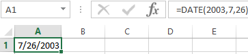
The example of DATE function

You need to describe of the date value with compiling it with individual elements of numbers.

There is the syntax: year; month, day.

All arguments are required. They can be specified by numbers or by reference to cells with the corresponding numeric data: for the year — from 1900 to 9999; for the month — from 1 to 12; for the day — from 1 to 31.

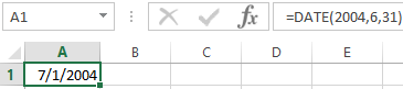
If you point a larger number for the «Day» argument (than the number of days in the pointed month), you receive the extra days, will be passed to the next month. For example, specifying 32 days for December, we will receive as a result on January 1.

The example of using the function:

Let’s set more days for June:

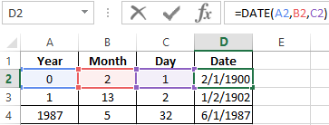
Examples of using the cell references as arguments:

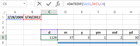
The DATEDIF function in Excel

It returns the difference between two dates.

The arguments:

• start date;
• final date;
• the code indicating to the units of counting (days, months, years, etc.).

The methods of measuring intervals between the given dates:

• to display the result in days — «d»;
• in months – «m»;
• in years – «y»;
• in months without years – «ym»;
• in days without months and years – «md»;
• in days without years – «yd».

In some versions of Excel, if you use the last two arguments («md», «yd»), the function may give an error. It is better to use to alternative formulas.

The examples of the operation the DATEDIF function:

In Excel 2007 version, this function is not in the directory, but it works. But you need to check the results are better, because there are flaws possible.

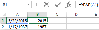
The YEAR function in Excel

It returns the year as an integer number (from 1900 to 9999), what corresponds to the specified date. There is only one argument must be entered in the structure of the function – is the date in a numerical format. The argument must be entered using the DATE function or represents to the result of evaluating other formulas.

The example of using the YEAR function:

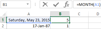
The MONTH function in Excel: the example

It returns the month as an integer number (from 1 to 12) for a date is specified in a numeric format. The argument – is the date of the month that you want to show in a numerical format. The dates in the text format this function does not handle correctly.

The examples of using the MONTH function:

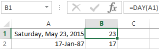
The examples of DAY, WEEKDAY and functions WEEKNUM in Excel

It returns the day as an integer number (from 1 to 31) for a date specified in a numeric format. The argument – it is the date of the day you want to find in a numerical format.

For returning of the weekday ordinal of the specified date, you can apply the function WEEKDAY:

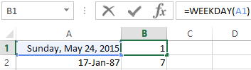
By default, the function considers Sunday the 1-st day of the week.

To display of the ordinal number of the week for the pointed date, you should use the WEEKNUM function:

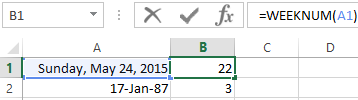
The date of 24. 05. 2015 is 22 week in a year. The week starts on Sunday (by default).

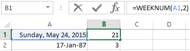
As the second argument the figure 2 is specified. Therefore, the formula considers that the week starts on Monday (the 2-d day of the week).

Download all examples functions for working with dates

For indicating of the current date, the function TODAY (no arguments) is used. To display the current time and date, the function NOW() is used.

WEEKDAY | NETWORKDAYS | WORKDAY | NETWORKDAYS.INTL | Fill Weekdays | WORKDAY.INTL | Highlight Weekdays

Use WEEKDAY, NETWORKDAYS and WORKDAY to create cool weekday formulas in Excel. Are you ready to improve your Excel skills?

WEEKDAY

The WEEKDAY function in Excel returns a number from 1 (Sunday) to 7 (Saturday) representing the day of the week of a date.

1. The WEEKDAY function below returns 2. 12/22/2025 falls on a Monday.

2. You can also use the TEXT function to display the day of the week.

3. Or create a custom date format (dddd) to display the day of the week. Cell A1 still contains a date.

NETWORKDAYS

The NETWORKDAYS function in Excel returns the number of workdays between two dates. NETWORKDAYS excludes weekends (Saturday and Sunday).

1. The NETWORKDAYS function below returns 11. There are 11 workdays between 12/17/2025 and 12/31/2025.

Explanation: the NETWORKDAYS function includes the start date and the end date. The calendar below helps you understand this formula. Simply count the number of circles.

2. If you supply a list of holidays, the NETWORKDAYS function also excludes holidays.

Explanation: simply count the number of circles in the calendar below.

WORKDAY

The WORKDAY function in Excel returns the date before or after a specified number of workdays. WORKDAY excludes weekends (Saturday and Sunday).

1. The WORKDAY function below returns the date 1/1/2026.

Explanation: the WORKDAY function does not include the start date. The calendar below helps you understand this formula. There are 11 circles.

2. If you supply a list of holidays, the WORKDAY function also excludes holidays.

Explanation: there are 11 circles in the calendar shown below.

NETWORKDAYS.INTL

Use NETWORKDAYS.INTL instead of NETWORKDAYS to specify different weekend days. Use a string of 0’s and 1’s (third argument) to specify which days are weekend days.

1. The NETWORKDAYS.INTL function below returns 8.

Explanation: the first 0 tells Excel that Monday is not a weekend day. The second 0 tells Excel that Tuesday is not a weekend day, etc. In this example, Friday, Saturday and Sunday are weekend days. The calendar below helps you understand this formula.

Fill Weekdays

To quickly create a list of dates excluding Saturdays and Sundays, execute the following steps.

1. For example, enter the date 12/17/2025 into cell A1.

2. Select cell A1 and drag the fill handle down. AutoFill automatically fills in the days.

3. Instead of filling in days, use the AutoFill options to fill in weekdays (ignoring weekend days).

Note: use WORKDAY.INTL to exclude different weekend days and holidays. Read on.

WORKDAY.INTL

Use WORKDAY.INTL instead of WORKDAY to specify different weekend days. Let’s create a list of dates excluding Mondays, Sundays and holidays.

1. Enter the date 12/17/2025 into cell A1 and specify a list of holidays (E1:E2).

2. Enter the WORKDAY.INTL function shown below.

Explanation: use a string of 0’s and 1’s (third argument) to specify which days are weekend days. The first 1 tells Excel that Monday is a weekend day. The second 0 tells Excel that Tuesday is not a weekend day, etc. In this example, Monday and Sunday are weekend days.

3. Select cell A2 and drag the fill handle down.

Explanation: the calendar below helps you understand this formula.

Conclusion: this formula automatically skips Mondays, Sundays and holidays. Pretty cool.

Highlight Weekdays

You can use conditional formatting in Excel to highlight dates that are weekdays (Monday, Tuesday, Wednesday, Thursday or Friday).

1. For example, select the range A1:A8.

2. On the Home tab, in the Styles group, click Conditional Formatting.

3. Click New Rule.

4. Select ‘Use a formula to determine which cells to format’.

5. Enter the formula =AND(WEEKDAY(A1)>1,WEEKDAY(A1)<7)

6. Select a formatting style and click OK.

Result. Excel highlights all weekdays.

Explanation: always write the formula for the upper-left cell in the selected range. Excel copies the formula to the other cells. Use the formula =OR(WEEKDAY(A1)=1,WEEKDAY(A1)=7) to highlight weekend dates.