
Excel for Microsoft 365 Excel for Microsoft 365 for Mac Excel for the web Excel 2021 Excel 2021 for Mac Excel 2019 Excel 2019 for Mac Excel 2016 Excel 2016 for Mac Excel 2013 Excel for Mac 2011 More…Less
This article describes the formula syntax and usage of the DAYS function in Microsoft Excel. For information about the DAY function, see DAY function.
Description
Returns the number of days between two dates.
Syntax
DAYS(end_date, start_date)
The DAYS function syntax has the following arguments.
-
End_date Required. Start_date and End_date are the two dates between which you want to know the number of days.
-
Start_date
Required. Start_date and End_date are the two dates between which you want to know the number of days.
Note: Excel stores dates as sequential serial numbers so that they can be used in calculations. By default, Jan 1, 1900 is serial number 1, and January 1, 2008 is serial number 39448 because it is 39447 days after January 1, 1900.
Remarks
-
If both date arguments are numbers, DAYS uses EndDate–StartDate to calculate the number of days in between both dates.
-
If either one of the date arguments is text, that argument is treated as DATEVALUE(date_text) and returns an integer date instead of a time component.
-
If date arguments are numeric values that fall outside the range of valid dates, DAYS returns the #NUM! error value.
-
If date arguments are strings that cannot be parsed as valid dates, DAYS returns the #VALUE! error value.
Example
Copy the example data in the following table, and paste it in cell A1 of a new Excel worksheet. For formulas to show results, select them, press F2, and then press Enter. If you need to, you can adjust the column widths to see all the data.
|
Data |
||
|---|---|---|
|
31-DEC-2021 |
||
|
1-JAN-2021 |
||
|
Formula |
Description |
Result |
|
=DAYS(«15-MAR-2021″,»1-FEB-2021») |
Finds the number of days between the end date (15-MAR-2021) and start date (1-FEB-2021). When you enter a date directly in the function, you need to enclose it in quotation marks. Result is 42. |
42 |
|
=DAYS(A2,A3) |
Finds the number of days between the end date in A2 and the start date in A3 (364). |
364 |
Top of Page
Need more help?
Want more options?
Explore subscription benefits, browse training courses, learn how to secure your device, and more.
Communities help you ask and answer questions, give feedback, and hear from experts with rich knowledge.
Функция DAY (ДЕНЬ) используется в Excel, для того чтобы узнать порядковый номер дня месяца (в промежутке от 1 до 31) из любой даты.
Содержание
- Что функция возвращает
- Синтаксис
- Аргументы функции DAY (ДЕНЬ) в Excel
- Дополнительная информация
- Примеры использования функции DAY (ДЕНЬ) в Excel
- Пример №1. Получаем значение дня используя числовой аргумент
- Пример №2. Получаем значение дня из ячейки с датой
- Пример №3. Получаем значение дня текущей даты
- Пример №4. Получаем значение первого дня месяца
Что функция возвращает
Возвращает число в промежутке от 0 до 31, в зависимости от даты, из которой требуется извлечь данные. Например, возвращая данные для Февраля, формула вернет номер дня в промежутке от «0» до «29».
Синтаксис
=DAY(serial_number)
=ДЕНЬ(дата_в_числовом_формате)
Аргументы функции DAY (ДЕНЬ) в Excel
- serial_number (дата_в_числовом_формате): Это порядковый номер дня. Он может быть результатом вычисления формулы, ссылкой на ячейку, которая содержит дату или данные введенные вручную.
Дополнительная информация
Помимо введенных в ручную чисел, функция DAY (ДЕНЬ) также будет работать с:
- результатами вычислений;
- датой введенной в текстовом формате (в кавычках);
- датой, указанной в текстовом формате;
- Excel отразит любую дату начиная с 1 Января 1900 года на Windows и с 1904 года на Mac.
Примеры использования функции DAY (ДЕНЬ) в Excel
Пример №1. Получаем значение дня используя числовой аргумент

На примере выше в качестве аргумента мы используем число “42736”. Это порядковый номер даты “1 января 2017”. Так как 1 января это первый день месяца, то результатом вычисления будет “1”.
Пример №2. Получаем значение дня из ячейки с датой
Больше лайфхаков в нашем Telegram Подписаться
На примере выше, функция принимает значение ячейки с конкретной датой и возвращает номер дня месяца этой даты. Обратите внимание, что если вы используете формат даты, который не распознается Excel, он покажет ошибку.
Пример №3. Получаем значение дня текущей даты
Вы можете легко получить текущее значение дня с помощью функции TODAY (СЕГОДНЯ) в качестве исходных данных. Функция TODAY (СЕГОДНЯ) возвращает текущую дату, а DAY (ДЕНЬ), в свою очередь, использует эти данные, чтобы вернуть порядковый номер дня этого месяца.
На примере выше, функция TODAY(СЕГОДНЯ) возвращает 12-02-2017. Функция DAY (ДЕНЬ) принимает значение функции TODAY (СЕГОДНЯ) как вводные данные и возвращает значение “12” как порядковый номер дня этого месяца.
Пример №4. Получаем значение первого дня месяца
Вы также можете вычислить значение первого дня любого месяца.
На примере выше, значение дня для даты в ячейке “A2” — “15-03-2017” равно “15”. Для того чтобы узнать номер первого дня месяца этой даты, нам нужно вычесть из нее значение дня (получим “0”, т.к. все даты хранятся в Excel как порядковые номера) и прибавить “1”, чтобы получить первый день месяца.
Обратите внимание, что даты в ячейках D2 и D3 отформатированы как даты. Может случиться так, что, когда вы используете эту формулу, вы можете получить серийный номер (например, “42795” за 1 марта 2017 года). Затем вы можете просто отформатировать его в качестве даты.
DAY in Excel
The Day function in Excel looks at a given date and figures out what day of the month it is. It then gives you a number from 1 to 31, representing the day. For example, if you have a date “April 16, 2023” in cell B1 and use the formula =DAY (B1), you will get the result as 16.
Excel has categorized the DAY function under the Date/Time function, a built-in function in Excel.
DAY Formula in Excel
The formula/syntax is:
where,
Date_value/serial_number – You must enter an Excel date with a serial number format.
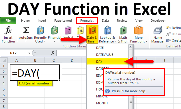
To access the Day function in Excel:
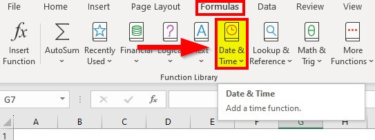
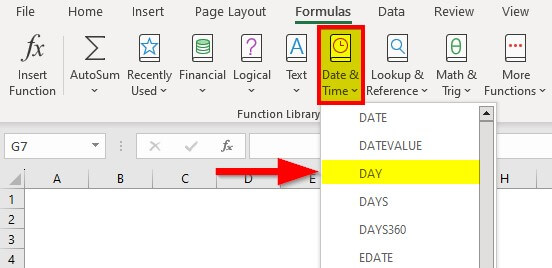
1. Click on the Formulas
2. Select the ‘Date & Time’ option.
3. Select the DAY function from the drop-down list.
How to Use DAY Function in Excel?
Example #1
Let’s say you have a list of dates in column A and want to extract only the day in another column, say column C.
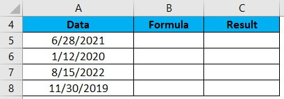
Here are the steps:
1. First, download the DAY Function Template. This template has all examples used in this article.
You can download this DAY Function Excel Template here – DAY Function Excel Template
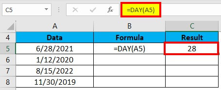
2. In cell C5, type the formula “=DAY(A5)” and press enter.
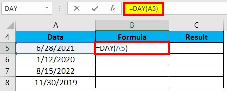
3. This will extract the day (28) from the date.
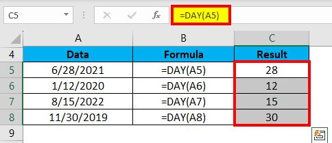
4. Drag and drop the formula from cell C5 to the remaining cells in column C to get the day for all the dates in column A.
5. Your result will be displayed in column C.
Example #2
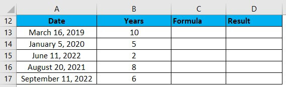
Suppose we have the below dates, and we need to add a given number of years to these dates. Let us use the DAY function to accomplish this:
We will enter this formula in cell C13: =DATE(YEAR(A13)+B13,MONTH(A13),DAY(A13))
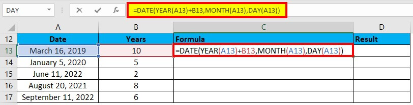
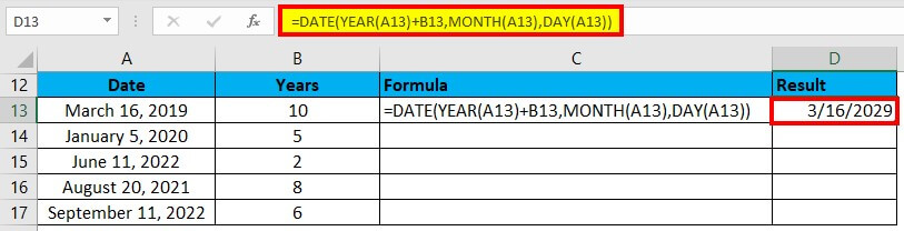
The formula provides the result as shown in the image below:
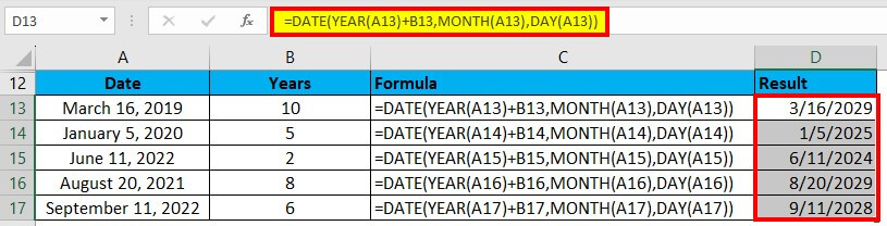
Drag & drop this formula to the remaining cells, and it gives the below result:
Explanation:
- The functions- YEAR, MONTH, and DAY that we used in the above formula retrieve the below data components:
For cell A13,
Year= 2019
Month= 3 (March)
Date= 16
Example #3
Suppose we want to find the first day of the month on a given date. For this, we will use the DAY function.
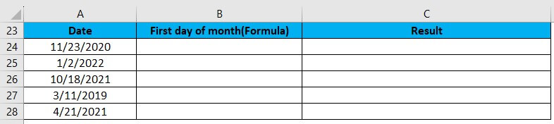
We will enter this formula in cell C24: =A24-DAY(A24)+1
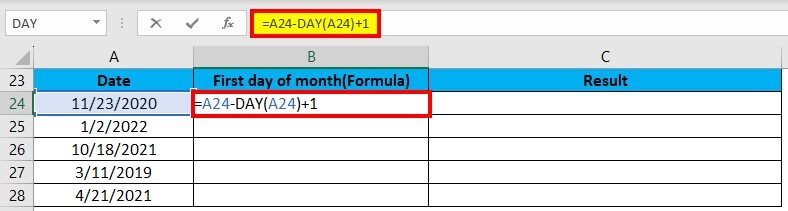
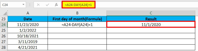
Excel provides the result as shown in the image below:
Drag & drop this formula for the rest values, and Excel provides the below result:
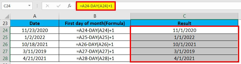
Explanation:
- The DAY function returns the day value for a date. The day value for the date 11/23/2020(cell A24) is 23.
- Excel stores the dates as serial numbers. So, we can subtract the value of 23 and then add 1 to obtain the date value for 11/01/2020.
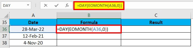
Example #4
We can calculate the number of days for a month on a given date with the help of the DAY function.

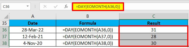
We will this formula: =DAY(EOMONTH(A36,0))
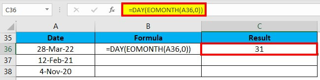
Drag & drop the formula to the remaining cells, which gives the results shown below:
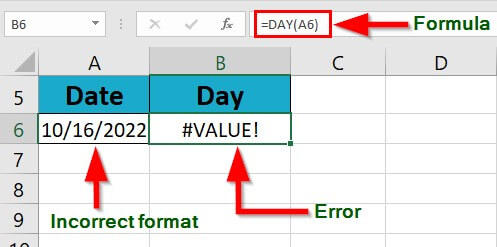
Common Errors and Fixes for Day in Excel
- #VALUE! – Excel gives a value error if we provide a date in the incorrect format, as shown below
To fix this error, follow these steps,
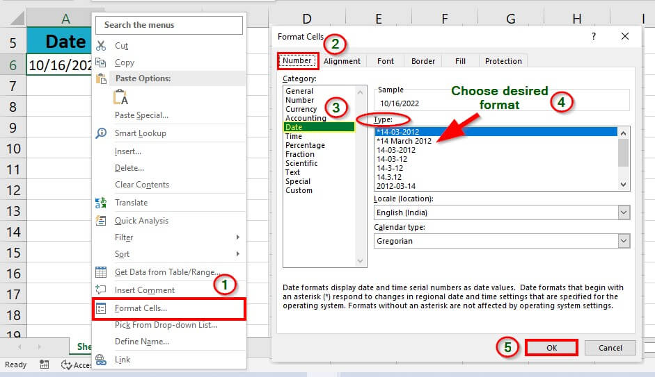
Step 1: Right-click the date, and choose Format Cells in the context menu
A Format Cells window pops up,
Step 2: Under the Format cells window, click Date under the Number tab, choose the desired date format from the list under the Type section, and click OK.
The entire process is illustrated in the image below.
Things to Remember
- The date argument must be a valid Excel date.
- Sometimes the DAY function provides a date- 01/01/1900, which looks like a date, while it needs to be an integer.
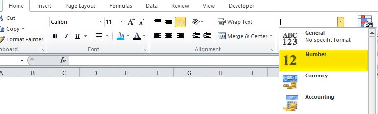
- To fix the above issue, go to the Number group in the Home tab and select Number from the various options. The process is illustrated in the following image.
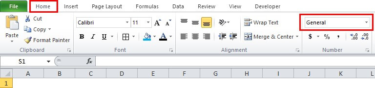
In the below image, select the Number option under General Option.
Frequently Asked Questions (FAQs)
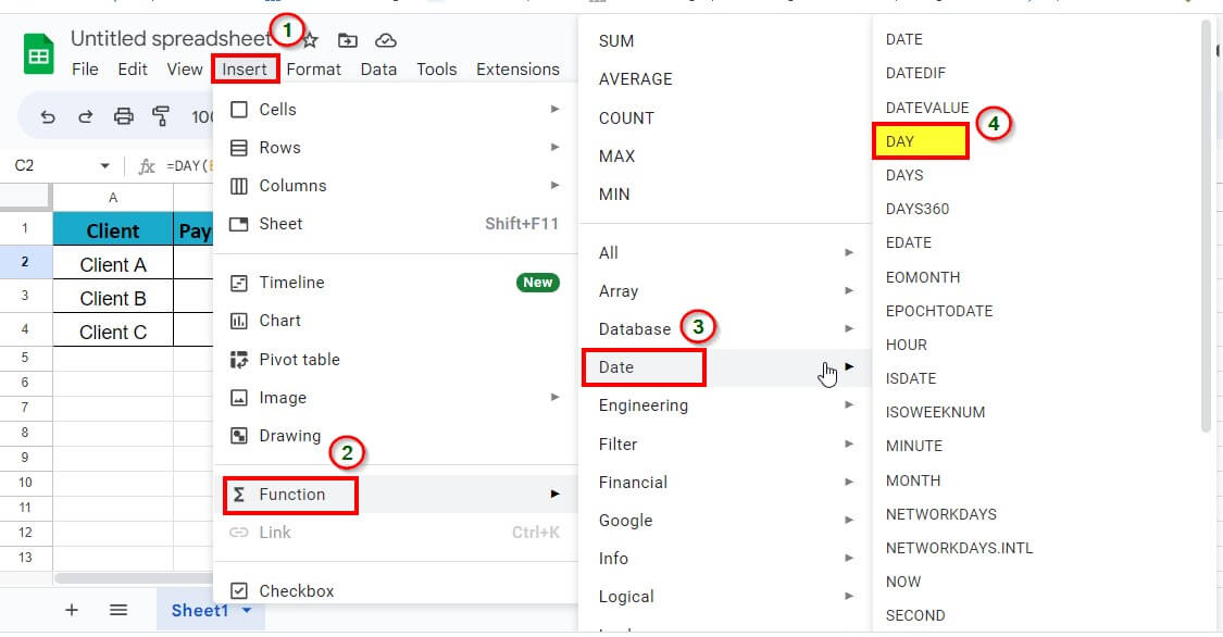
Q1. How do I use the day formula in Google Sheets?
Answer: To use the day formula in Google Sheets, follow these steps:
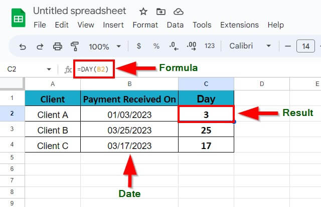
Step 1: Place the cursor in the cell where you want to display the Day and enter the formula =DAY(date)
Step 2: Hit Enter key to get the result
Alternatively,
You can insert the Day function by following these steps:
Insert > Function > Date > Day
Q2. How do I add a day in Google Sheets?
Answer: To add a given number of days to a date in Google Sheets, perform an addition of the two cells, i.e., use the formula = date + number of days.
Recommended Articles
The above article has been a guide to DAY in Excel. Here we discuss the DAY function in Excel and the way of using the DAY function along with downloadable Excel templates. EDUCBA recommends the following useful functions in Excel –
- $ in Excel
- Excel Search Box
- HLOOKUP in Excel
- VLOOKUP Function in EXCEL
Sample Files
1. DATE Function
DATE function returns a valid date based on the day, month, and year you input. In simple words, you need to specify all the components of the date and it will create a date out of that.
Syntax
DATE(year,month,day)
Arguments
- year: A number to use as the year.
- month: A number to use as the month.
- day: A number to use as a day.
Example
In the below example, we have used cell references to specify the year, month, and day to create a date.

You can also insert arguments directly into the function to create a date as you can see in the below example.

And in the below example, we have used different types of arguments to see the result returned by the function.

2. DATEVALUE Function
DATEVALUE function returns a date after converting a text (which represents a date) into an actual date. In simple words, it converts a date into an actual date which is formatted as text.
Syntax
DATEVAUE(date_text)
Arguments
- date_text: The date which is stored as a text and you want to convert that text into an actual date.
Example
In the below example, we have inserted a date directly into the function by using double quotation marks. If you skip adding these quotation marks it will return a #NAME? error in the result.

In the below example, all the dates on the left side are in textual format.
- A simple textual date that we have converted into a valid date.
- A date with all three components (Year, Month, or Day) in numbers.
- If there is no year in the textual date, it will take the current year as the year.
- And if you have a month name is in alphabets and no year, it will take the current year as a year.
- If you don’t have the day in your textual date it will take 1 as the day number.

3. DAY Function
DAY function returns the day number from a valid date. As you know, in Excel, a date is a combination of day, month, and year, DAY function gets the day from the date and ignores the rest of the part.
Syntax
DAY(serial_number)
Arguments
- serial_number: A valid serial number of the date from which you want to extract the day number.
Example
In the below example, we have used the DAY to simply get the day from a date.

And in the below example, we have used DAY with TODAY to create a dynamic formula that returns the current day number and it will update every time you open your worksheet or when you recalculate your worksheet.

5. DAYS Function
DAYS function returns the difference between two dates. It takes a start date and an end date and then returns the difference between them in days. This function was introduced in Excel 2013 so not available in prior versions.
Syntax
DAYS(end_date,start_date)
Arguments
- start_date: It is a valid date from where you want to start the days’ calculation.
- end_date: It is a valid date from where you want to end the days’ calculation.
Example
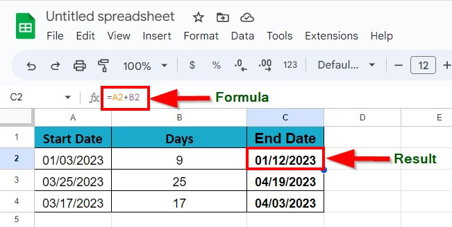
In the below example, we have referred the cell A1 as the start date and B1 as the end date and we have 9 days in the result.
Note: You can also use the subtract operator to get the difference between two dates.

In the below example, we have directly inserted two dates into the function to get the difference between them.

6. EDATE Function
EDATE function returns a date after adding a specified number of months to it. In simple words, you can add (with a positive number) or subtract (with a negative number) months from a date.
Syntax
EDATE(start_date,months)
Arguments
- start_date: The date from which you want to start the calculation.
- months: The number of months to calculate the future or the past date.
Example
Here we have used EDATE with different types of arguments.
- In the first example, we have used 5 as a several months and it has added exactly 5 months on 1-Jan-2016 and returned 01-June-2016.
- In the second example, we have used -1 month and it has given 31-Dec-2016, a date which is exactly 1 month back from 31-Jan-2016.
- In the third example, we have inserted a date directly into the function.

7. EOMONTH Function
EOMONTH function returns the end of the month date which is the number of months in the future or the past. You can use a positive number for a future date and a negative number for the past month’s date.
Syntax
EOMONTH(start_date,months)
Arguments
- start_date: A valid date from where you want to start your calculation.
- months: The number of months you want to calculate before and after the start date.
Example
In the below example, we have used EOMONTH with different types of arguments:

- We have mentioned 01-Jan-2016 as the start date and 5 months for getting a future date. As June is exactly 5 months after January, it has returned 30-Jun-2016 in the result.
- As I have already mentioned, EOMMONTH is smart enough to evaluate the total number of days in a month.
- If you mention a negative number, it simply returns a past date which is the number of months back you have mentioned.
- In the fourth example, we have used a date that is in text format and it has returned the date without returning any errors.
8. MONTH Function
MONTH function returns the month number (ranging from 0 to 12) from a valid date. As you know, in Excel, a date is a combination of day, month, and year, MONTH gets the month from the date and ignores the rest of the part.
Syntax
MONTH(serial_number)
Arguments
- serial_number: A valid date from which you want to get the month number.
Example
In the below example, we have used a MONTH in three different ways:

- In the FIRST example, we have simply used date and it has returned the 5 in the result which is the month number of MAY.
- In the SECOND example, we have supplied the date directly in the function.
- In the THIRD example, we have used the TODAY function to get the current date and MONTH has returned the month number from it.
9. NETWORKDAYS Function
NETWORKDAYS function returns the count of days between the start date and end date. In simple words, with NETWORKDAYS you can calculate the difference between two dates, after excluding Saturdays and Sundays, and holidays (which you specify).
Syntax
NETWORKDAYS(start_date,end_date,holidays)
Arguments
- start_date: A valid date from where you want to start your calculation.
- end_date: A valid date up to which you want to calculate working days.
- [holidays]: A valid date that represents a holiday between the start date and end date. You can refer to a cell, range of cells, or an array containing dates.
Example
In the below example, we have specified 10-Jan-2015 as a start date and 20-Feb-2015 as an end date.

We have 41 days between these two dates, out of which 11 days are weekends. After deducting those 11 days it has returned 30 working days.
Now in the below example with the same start and end dates, we have specified a holiday and, after deducting 11 days of the weekend and 1 holiday it has returned 29 working days.

Again with the same start and end dates, we have used a range of three cells for holidays to deduct from the calculation and, after deducting 11 weekend days and 3 holidays which I have mentioned It has returned 27 working days.

10. NETWORKDAYS.INTL Function
NETWORKDAYS.INTL Function returns the count of days between the start date and end date. Unlike NETWORKDAYS, NETWORKDAYS.INTL lets you specify which days you want to exclude from the calculation.
Syntax
NETWORKDAYS.INTL(start_date,end_date,weekend,holidays)
Arguments
- start_date: A valid date from where you want to start your calculation.
- end_date: A valid date up to which you want to calculate working days.
- [weekend]: A number represents to exclude weekends from the calculation.
- [holidays]: A list of dates that represents the holidays you want to exclude from the calculation.
Example
In the below example, we have used 01-Jan-2015 as a start date and 20-Jan-2015 as an end date. And we have specified 1 to take Sunday – Saturday as the weekend. The function has returned 14 days after excluding 6 weekend days.

Below, we have used the same dates. And I have used 11 in for weekend days which means it will only consider Sunday as a weekend. Along with that, we have also used 10-Jan-2015 as a holiday.

We have 3 Sundays between both dates and a holiday. After excluding all these days the function has returned 16 days in the result. Here in the below example, we have used range to specify holidays. If you have more than one date for the holidays you can refer to an entire range.

Quick Tip: If you want to create a dynamic range for holidays, you can use a table for that. If you want to choose custom days to count as working days or weekends, you can use the below format in the weekend argument.

Here, 0 represents a working day and 1 represents a non-working day. And, seven numbers represent 7 days of the week.
11. TODAY Function
The TODAY function returns the current date and time as per the system’s date and time. The date and time returned by the NOW function update continuously whenever you update anything in the worksheet.
Syntax
TODAY()
Arguments
- In the TODAY function, there is no argument, all you need to do is enter it in the cell and hit enter, but be careful as TODAY is a volatile function which updates its value every time you update your worksheet calculations.
Example
In the below example, we have used TODAY with other functions to get the current month number, current year, and current day.

12. WEEKDAY Function
WEEKDAY function returns a day number (ranging from 0 to 7) of the week from a date. In simple words, the WEEKDAY function takes a date and returns the day number of that date’s day.
Syntax
WEEKDAY (serial_number, [return_type])
Arguments
- serial_number: A valid date from which you want to get the week number.
- [return_type]: A number that represents the day of the week to start the week.
Example
In the below example, we have used a WEEKDAY with TODAY to get a dynamic weekday. It will give you the weekday whenever the current date changes. You can use this method in your dashboards to trigger some values which need to change when weekday change.

In the below example, we have used WEEKDAY with IF to create a formula that first checks the weekday of date and return “Weekday” or “Weekend” basis on the value return from WEEKDAY.

13. WEEKNUM Function
WEEKNUM function returns the week number of a date. In simple words, WEEKNUM returns the week number of dates that you specify ranging from 1 to 54.
Syntax
WEEKNUM(serial_number,return_type)
Arguments
- serial_number: A date for which you want to get the week number.
- [return_type]: A number to specify the starting day of the first week of the year. You have two systems to specify the starting date of the week.
Example
In the below example, we have used TODAY with WEEKNUM to get the week number of the current date. It will update the week number automatically every time the date changes.

In the below example, we have added the text “Week-” with the week number for a meaningful result.

14. YEAR Function
YEAR Function returns the year number from a valid date. As you know, in Excel a date is a combination of day, month, and year, and the YEAR function gets the year from the date and ignores the rest of the part.
Syntax
YEAR(date)
Arguments
- date: A date from which you want to get the year.
Example
In the below example, we have used the year function to get the year number from the dates. You can use this function where you have dates in your data and you only need the year number.

And in the below example, we have used today function to get the year number from the current date. It will always update the year whenever you recalculate your worksheet.
