Day in words excel - Word и Excel - помощь в работе с программами

Содержание

Convert Date into words in Excel
How to Convert Date into words in Excel
The DATEDIF formula
Syntax and Arguments of DATEDIF formula
Translate Date into other Language – convert date into words in Excel
How to convert date to text in Excel with TEXT function and without formulas
Using TEXT function in Excel to convert date to text
Example 1. How to convert date to text strings in different formats
Example 2. How to convert time to text strings
Example 3. How to convert the current date to text in Excel
Example 4. Excel TEXT formula to convert text to date
Converting date to text with Excel’s Text to Columns wizard
Convert Excel date to text via Notepad

Convert Date into words in Excel

Convert date into words in Excel – Microsoft Excel is a powerful tool for numbers to text, numbers to words, get a date of birth, convert date to string, convert date of birth in words, convert date to text month, convert date to words, get age in word, and convert date to text.

How to Convert Date into words in Excel

In order to convert a date into words in Excel, the easy way to understand the working of MS Excel formula just separate years, months, and days from the date. While converting the data into words in Excel, will help you to understand the logic.

The below figure of convert a date into words in Excel is showing that A1 cell text is Date of Birth, B1 cell text is Year, C1 Months, D1 Days, and E1 cell has text Age in Words.

convert a date into words in Excel

convert a date into words in Excel – Now we will type any date of birth to convert into words in cell A2. I am using the format of date is as “DD-MM-YYYY”, so I will enter first DD, MM, and YYYY. and you may be using the date format as “MM-DD-YYYY” and you will enter your date according to your format. The format represents MM = months, DD = days, and YYYY as years.

The DATEDIF formula

The DATEDIF formula is used to extract years, months and days. Microsoft Excel doesn’t provide any preview or help when you start type formula in the cell. So, you should be careful while using the formula. Using the DATEDIF formula you can get years, months, and days between two dates. The DATEDIF formula provides you a simple and easy way to get differences between two dates or get age from a date to date.

Syntax and Arguments of DATEDIF formula

=DATEDIF (start-date, end-date, unit)
Start-date – The first or start date.
End-date – the last or ending or the current date.
unit – get years only type “y” or months only “ym” or days on “md”.

Type formula in B2 to extract a number of years from A2. The above discussion shows that the first parameter is the start date, the second is the last or current date, and finally is unit. For the current date, we will use TODAY () formula to get the current time of the system, and in units, we will use “y” for years, “ym” for months, and “md” for days. See the below formulas, which are going to use the Excel sheet.

Now we got Years, Months, and Days in different cells from a cell A1. When you type a new date, MS Excel will automatically separate years, months, and days in formulated cells. The last step of convert date into words in Excel is to apply to choose formula. Just copy and paste the following formula into E2 cell and hit the enter key.

You will see the number of B2 is converted into words. This is the main formula to convert numbers into text for date management. Now append &” Years “at the end of the pasted formula, now you will the text is changed into “Thirty Seven Years”

The next step is to add months to E2 cell. In the above formula just copy it into Notepad, and replace = sign with & and replace B2 cell name with C2 and “ Years” with “ Months “ &

Now append the above formula with already existing formula in E2 cell. When you press Enter key it should show “Thirty-seven Years Eleven Months and ”. The final step of convert date into words in Excel is to add days string into E2. The method is the same as repeated with months, just replace C2 with D2 and “Months and “ with “Days”

Translate Date into other Language – convert date into words in Excel

The translation of words, lines, and paragraphs is a great feature in Microsoft Office. You can use this feature under the “Review” tab in Microsoft Word, Excel, PowerPoint, and other MS Office. But the translation into other language matters, either it is translating with correct words or not.

Microsoft Office can translate text into different languages, but it has some issues. While I was working over date translation into other languages, I found that if the date is March 7, 2020, in English words it should seven march and twenty thousand twenty, and in the Urdu language, it should “سات مارچ بیس سو بیس” But it was showing “2020 سات مارچ”. This was the issue in Microsoft language translation.

Google translator is very good and close to human translation. It is absolutely free and easy to use. Google translator another plus point it is fast than Microsoft translator.

[Download file with Report card]

Topic Name: Convert a date into words in Excel

The theme of Convert date into words in Excel article

Convert a date into words in Excel – So hope you got some useful information about numbers to text in excel, numbers to words in excel, get the date of birth in excel, choose formula in excel, left formula in excel, dob in excel, separate days months years in excel, DATEDIF formula.

You can watch the video to understand how to convert a date into words in Excel, Please like, comment, and share the video. Thanks for watching the video.

Источник

How to convert date to text in Excel with TEXT function and without formulas

by Svetlana Cheusheva, updated on February 7, 2023

In the previous article, we discussed different ways to convert text to date in Excel. If you are looking for a solution to the opposite task — changing an Excel date to text — a few choices are available to you again.

Traditionally, we’ll begin with a formula solution and then explore a couple of non-formula ways.

Using TEXT function in Excel to convert date to text

The Excel TEXT function is specially designed to convert a numeric value to a text string and display it in the format you specify.

The syntax of the Excel TEXT function is as follows:

value is a numeric value you want to convert to text. This can be a number, a formula that returns a numeric value, or a reference to a cell containing a number.
format_text this is how you want to format the resulting text value, provided as a text string enclosed in quotation marks.

For example, you can use the following formula to convert a date in cell A1 to a text string in the traditional US date format (month/day/year):

=TEXT(A1,»mm/dd/yyyy»)

As you see in the screenshot above, the value returned by the TEXT formula is aligned to the left, which is the first sign that points to a date formatted as text. Apart from alignment in a cell, there are a few more indicators that can help you distinguish between dates and text strings in Excel.

Example 1. How to convert date to text strings in different formats

Since Excel dates are serial numbers in their nature, the Excel TEXT function has no problem with converting them to text values. The most challenging part is probably specifying the proper display formatting for the text dates.

Microsoft Excel understands the following date codes.

m — month number without a leading zero
mm — month number with a leading zero
mmm — short form of the month name, for example Mar
mmmm — full form of the month name, for example March
mmmmm — month as the first letter, for example M (stands for March and May)

d — days number without a leading zero
dd — day number with a leading zero
ddd — abbreviated day of the week, for example Sun
dddd — full name of the day of the week, for example Sunday

yy — two-digit year
yyyy — four-digit year

To display the converted text date exactly the way you want, you can separate the date codes with various delimiters such as dash (-), slash (/), comma (,) colon (:), etc. Here are a few examples:

«mm/dd/yyyy» — the date format used in the USA, displays as 03/08/2015
«dd/mm/yyyy» — the date format used by the rest of the world, displays as 08/03/2015
«dd-mmm-yy» — displays as 08-Mar-15 to avoid any confusion : )
«dddd, mmmm d, yyyy» — full date, including the day of the week, displays as Sunday, March 08, 2015

For example, if you have a column of US dates in Excel and you need to export them to a .csv file for your UK based partner, you can convert the dates to the UK format, as a courtesy:

Some more formula examples and their results are shown below: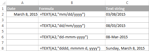

Example 2. How to convert time to text strings

If your date entries display both dates and times and you want to change them to text strings exactly as they are, you included the following time codes in the format_text argument of the Excel TEXT function.

h — hours without a leading zero, as 0-23.
hh — hours with a leading zero, as 00-23.

m — minutes without a leading zero, as 0-59
mm — minutes with a leading zero, as 00-59

s — seconds without a leading zero
ss — seconds with a leading zero

Periods of the day:

AM/PM — displays as AM or PM
If not specified, 24-hour time format is used

As you probably noticed, the m codes are used for months as well as minutes, and you might be curious how Microsoft Excel distinguishes between them. If you put «m» immediately after h codes (hours) or immediately before s codes (seconds), Excel understands you want to display minutes rather than a month. Yep, it’s that simple : )

The TEXT function in Excel allows including both date and time codes in the format_text argument, for example:

If you want to convert the time portion only, then put only the time codes, like this:

The results of your TEXT formulas may look similar to this: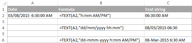

Example 3. How to convert the current date to text in Excel

In case you want to convert the current date to the text format, you can use the Excel TEXT function in combination with the TODAY function that returns the current date, for example:

The result of this formula would show up as 08-Mar-2015. If you prefer to display the resulting text string in some other format, please see the date codes discussed in Example 1.

Example 4. Excel TEXT formula to convert text to date

Though the main destination of the TEXT function in Excel is converting numbers to text, it can also perform a reverse conversion, i.e. change text to date. For this, you simply add the double negation (—) to your TEXT formula.

For example, to convert a text string in cell A1 to date, you use the below formula, and then format the cell as a date.

=—TEXT(A1,»mm/dd/yy»)

Note. In the above examples, we used the date and time codes for the English locale of Excel. If you have a different locale, the codes may be different for your language.

Converting date to text with Excel’s Text to Columns wizard

As you’ve just seen, Excel’s TEXT function makes a good job of converting dates to text. But if you are not a big fan of Excel formulas, you might like this solution better.

If you had a chance to read the previous part of our Excel dates tutorial, you already know how to use Text to Columns to change text to date. To convert dates to text strings, you proceed in the same way with the only difference that you choose Text instead of Date on the final step of the wizard.

Note. The Text to Column wizard always converts dates in the default short date format regardless of how the original dates are displayed in your worksheet. You can find more about default date and time formats in the following article: Default date format in Excel.

If the default date format is not what you are looking for, you can jump right to the next solution that lets you convert dates to text strings in any format of your choosing.

If you don’t mind the default format, then perform the following steps:

In your Excel spreadsheet, select all of the dates you want to change to text.
On the Data tab, find the Data Tools group, and click Text to Columns.
On step 1 of the wizard, select the Delimited file type and click Next.
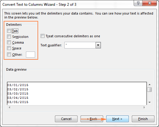
On step 2 of the wizard, make sure none of the delimiter boxes is checked and click Next.
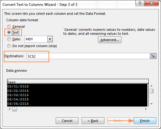
On step 3 of the wizard, which is the final step, select Text under Column data format and click Finish.

Tip. If you don’t want the resulting text strings to overwrite the original dates, specify the Destination for the top cell of the new column.

That was really easy, right? The screenshot below demonstrates the result — dates converted to text strings in the default short date format set in your Windows Regional settings, which is «mm/dd/yyyy» in my case:

Convert Excel date to text via Notepad

Another quick no-formula way to turn Excel dates into text strings is using Notepad or any other text editor. Unlike the Text to Columns wizard, it allows you to convert Excel date to text in any format of your choosing.

In your Excel worksheet, format the dates exactly as you want the text strings to look like.
Select all of the dates you want to convert and press Ctrl+C to copy them.
Open Notepad or any other text editor, and paste the copied dates there.
Notepad automatically converts the dates to the text format. Press Ctrl+A to select all text strings, and then Ctrl+C to copy them.
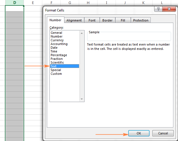
Switch back to Microsoft Excel, select the column where you want to insert the text strings and apply the Text format to it. To do this, press Ctrl+1 to open the Format Cells dialog and select Text on the Number tab.
Finally, select the first cell where you want to insert the text strings and press Ctrl+V to paste them.

The following screenshot shows the result, with the original Excel dates in column B and text entries in column D. Please notice that the converted text strings reflect the original date format with absolute accuracy, except they are left-alighted, as all text values are supposed to be in Excel.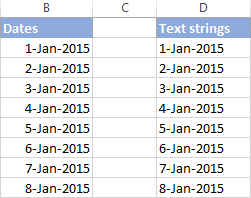

This is how you convert date to text in Excel. Next week we will explorer a few Excel functions to work with weekdays and days of the year. And in the meantime, you may want to check out the previous parts of our comprehensive tutorial to working with dates and times in Excel.

Источник

How to Convert Date into words in Excel

The below figure of convert a date into words in Excel is showing that A1 cell text is Date of Birth, B1 cell text is Year, C1 Months, D1 Days, and E1 cell has text Age in Words.

convert a date into words in Excel

The DATEDIF formula

Syntax and Arguments of DATEDIF formula

=DATEDIF (start-date, end-date, unit)
Start-date – The first or start date.
End-date – the last or ending or the current date.
unit – get years only type “y” or months only “ym” or days on “md”.

=DATEDIF(A2,TODAY(),”y”)
=DATEDIF(A2,TODAY(),”ym”)
=DATEDIF(A2,TODAY(),”md”)

=CHOOSE(LEFT(TEXT(B2,"000"))+1,,"One","Two","Three","Four","Five","Six","Seven","Eight","Nine")
&IF(--LEFT(TEXT(B2,"000"))=0,,IF(AND(--MID(TEXT(B2,"000"),2,1)=0,--MID(TEXT(B2,"000"),3,1)=0)," Hundred"," Hundred and "))
&CHOOSE(MID(TEXT(B2,"000"),2,1)+1,,,"Twenty ","Thirty ","Forty ","Fifty ","Sixty ","Seventy ","Eighty ","Ninety ")
&IF(--MID(TEXT(B2,"000"),2,1)<>1,CHOOSE(MID(TEXT(B2,"000"),3,1)+1,,"One","Two","Three","Four","Five","Six","Seven","Eight","Nine"),
CHOOSE(MID(TEXT(B2,"000"),3,1)+1,"Ten","Eleven","Twelve","Thirteen","Fourteen","Fifteen","Sixteen","Seventeen","Eighteen","Nineteen"))

=CHOOSE(LEFT(TEXT(B2,"000"))+1,,"One","Two","Three","Four","Five","Six","Seven","Eight","Nine")
&IF(--LEFT(TEXT(B2,"000"))=0,,IF(AND(--MID(TEXT(B2,"000"),2,1)=0,--MID(TEXT(B2,"000"),3,1)=0)," Hundred"," Hundred and "))
&CHOOSE(MID(TEXT(B2,"000"),2,1)+1,,,"Twenty ","Thirty ","Forty ","Fifty ","Sixty ","Seventy ","Eighty ","Ninety ")
&IF(--MID(TEXT(B2,"000"),2,1)<>1,CHOOSE(MID(TEXT(B2,"000"),3,1)+1,,"One","Two","Three","Four","Five","Six","Seven","Eight","Nine"),
CHOOSE(MID(TEXT(B2,"000"),3,1)+1,"Ten","Eleven","Twelve","Thirteen","Fourteen","Fifteen","Sixteen","Seventeen","Eighteen","Nineteen")) & " Years "

The next step is to add months to E2 cell. In the above formula just copy it into Notepad, and replace = sign with & and replace B2 cell name with C2 and “ Years” with “ Months “ &

& CHOOSE(LEFT(TEXT(C2,"000"))+1,,"One","Two","Three","Four","Five","Six","Seven","Eight","Nine")
&IF(--LEFT(TEXT(C2,"000"))=0,,IF(AND(--MID(TEXT(C2,"000"),2,1)=0,--MID(TEXT(C2,"000"),3,1)=0)," Hundred"," Hundred and "))
&CHOOSE(MID(TEXT(C2,"000"),2,1)+1,,,"Twenty ","Thirty ","Forty ","Fifty ","Sixty ","Seventy ","Eighty ","Ninety ")
&IF(--MID(TEXT(C2,"000"),2,1)<>1,CHOOSE(MID(TEXT(C2,"000"),3,1)+1,,"One","Two","Three","Four","Five","Six","Seven","Eight","Nine"),
CHOOSE(MID(TEXT(C2,"000"),3,1)+1,"Ten","Eleven","Twelve","Thirteen","Fourteen","Fifteen","Sixteen","Seventeen","Eighteen","Nineteen")) & " Months and "

=CHOOSE(LEFT(TEXT(B2,"000"))+1,,"One","Two","Three","Four","Five","Six","Seven","Eight","Nine")
&IF(--LEFT(TEXT(B2,"000"))=0,,IF(AND(--MID(TEXT(B2,"000"),2,1)=0,--MID(TEXT(B2,"000"),3,1)=0)," Hundred"," Hundred and "))
&CHOOSE(MID(TEXT(B2,"000"),2,1)+1,,,"Twenty ","Thirty ","Forty ","Fifty ","Sixty ","Seventy ","Eighty ","Ninety ")
&IF(--MID(TEXT(B2,"000"),2,1)<>1,CHOOSE(MID(TEXT(B2,"000"),3,1)+1,,"One","Two","Three","Four","Five","Six","Seven","Eight","Nine"),
CHOOSE(MID(TEXT(B2,"000"),3,1)+1,"Ten","Eleven","Twelve","Thirteen","Fourteen","Fifteen","Sixteen","Seventeen","Eighteen","Nineteen")) & " Years " 
& CHOOSE(LEFT(TEXT(C2,"000"))+1,,"One","Two","Three","Four","Five","Six","Seven","Eight","Nine")
&IF(--LEFT(TEXT(C2,"000"))=0,,IF(AND(--MID(TEXT(C2,"000"),2,1)=0,--MID(TEXT(C2,"000"),3,1)=0)," Hundred"," Hundred and "))
&CHOOSE(MID(TEXT(C2,"000"),2,1)+1,,,"Twenty ","Thirty ","Forty ","Fifty ","Sixty ","Seventy ","Eighty ","Ninety ")
&IF(--MID(TEXT(C2,"000"),2,1)<>1,CHOOSE(MID(TEXT(C2,"000"),3,1)+1,,"One","Two","Three","Four","Five","Six","Seven","Eight","Nine"),
CHOOSE(MID(TEXT(C2,"000"),3,1)+1,"Ten","Eleven","Twelve","Thirteen","Fourteen","Fifteen","Sixteen","Seventeen","Eighteen","Nineteen")) & " Months and " 
& CHOOSE(LEFT(TEXT(D2,"000"))+1,,"One","Two","Three","Four","Five","Six","Seven","Eight","Nine")
&IF(--LEFT(TEXT(D2,"000"))=0,,IF(AND(--MID(TEXT(D2,"000"),2,1)=0,--MID(TEXT(D2,"000"),3,1)=0)," Hundred"," Hundred and "))
&CHOOSE(MID(TEXT(D2,"000"),2,1)+1,,,"Twenty ","Thirty ","Forty ","Fifty ","Sixty ","Seventy ","Eighty ","Ninety ")
&IF(--MID(TEXT(D2,"000"),2,1)<>1,CHOOSE(MID(TEXT(D2,"000"),3,1)+1,,"One","Two","Three","Four","Five","Six","Seven","Eight","Nine"),
CHOOSE(MID(TEXT(D2,"000"),3,1)+1,"Ten","Eleven","Twelve","Thirteen","Fourteen","Fifteen","Sixteen","Seventeen","Eighteen","Nineteen")) & " Days "

Translate Date into other Language – convert date into words in Excel

Google translator is very good and close to human translation. It is absolutely free and easy to use. Google translator another plus point it is fast than Microsoft translator.

[Download file with Report card]

Topic Name: Convert a date into words in Excel

The theme of Convert date into words in Excel article

You can watch the video to understand how to convert a date into words in Excel, Please like, comment, and share the video. Thanks for watching the video.

Источник

How to display the Excel day of the week from a date with a simple formula?

With the Excel software, it is more convenient to display the Excel day of the week in all letters rather than the date in a numeric Date format. Indeed, when using dates with Microsoft Office and especially Excel to manage statistics and schedules tables, readability is important. So, how to display Excel weekday in letters from a date with a simple formula?

The date format of the day/month/year type in numeric, like for example “30/11/2017” is not the easiest to read to analyse data. Especially with days less than or equal to 12, because the month can be confused with the day. And the Anglo-Saxon format uses month/day/year instead, which can give dates like 11/11/2011. So here is how to convert the date to day name in Excel.

These two following concrete examples allow you to display the weekday written in all letters for the first case, or only the first three letters for the second option.

1. Display the Excel weekday name in all letters

To display the Excel day of the week in all letters, one solution is to use the TEXT() Excel function with the day parameter on four letters: “dddd”. Simply add a formula in a cell, use the Text() function. Then add the TODAY() keyword as the first argument and the “dddd” as the second argument for the function.

=TEXT(TODAY(),"dddd")

2. Display the weekday from another cell in full letter

For example if the date to display in A1 cell, this formula do not use the current date with a time function, instead, is simply take a date, static or not, from another cell in the Excel Sheet.

=TEXT(A1,"dddd")

The result is Saturday for 01/01/2022 in A1. So, this formula will display the name of the day in all letters. That is to say the complete day. In this example the column will have the following format: Thursday

The formula arguments are from an English (UK) version of MS Excel, the syntax may vary depending on local language settings.

3. Display the Excel day of the week abbreviated in three letters

In other words, to display only the first three letters of the day, you have to use the TEXT() function with the keyword “dd”. Of course, if your source value is in another cell, then use the cell reference, here it is A1 in the second formula.

=TEXT(TODAY(),"ddd")

Display the excel day of the week from current date

The result is Sat for Saturday. Use also this variation to get the date from another cell.

=TEXT(A1,"ddd")

Display the excel day of the week from another cell using the TEXT formula

In addition, the list of days of the week with the formula that uses the three letters keyword will display the abbreviated days as below:

4. Excel formula to convert the day name to uppercase

Let’s convert today’s date into letters with Excel in uppercase this time. Always use the TEXT() formula, but this time with the parameter in uppercase: DDDD, as in this example it will display THURSDAY.

=TEXT(TODAY(),"DDDD")

5. Conclusion on displaying weekdays using Excel formulas

In conclusion, displaying the Excel day of the week in all letters or abbreviated form can greatly improve data readability. Simple formulas like TEXT() with the appropriate parameters can convert dates to the day name in Excel. You can use these formulas to display the day from a static or dynamic cell, or convert it to uppercase. Give them a try to save time and hassle when working with dates in your spreadsheets. They can help you better analyze your data and manage your schedules.

Note that this TEXT function also allows you to manage the format for different information. Among others: hours, weeks, months, and years but also percentages. And also, currencies with the symbol euro (€) or dollar ($) for example. To go further, here is a short MS Office tutorial on how to select an entire column in Excel using a shortcut.

Источник

Watch video – Convert Date to Text in Excel

Date and Time in Excel are stored as numbers. This enables a user to use these dates and time in calculations. For example, you can add a specific number of days or hours to a given date.

However, sometimes you may want these dates to behave like text. In such cases, you need to know how to convert the date to text.

Below is an example where dates are combined with text. You can see that the dates don’t retain their format and show up as numbers in the combined text.

In such situations, it’s required to convert a date into text.

Convert Date to Text in Excel

In this tutorial, you’ll learn three ways to convert the date to text in Excel:

Using the Text Function
Using the Text to Column feature
Using the Copy-Paste method

Convert Date to Text using Text Function

TEXT function is best used when you want to display a value in a specific format. In this case, it would be to display the date (which is a number) in the date format.

Let’s first see how the text function works.

Here is the syntax:

=TEXT(value, format_text)

It takes two arguments:

value – the number that you want to convert into text. This can be a number, a cell reference that contains a number, or a formula result that returns a number.
format_text – the format in which you want to display the number. The format needs to be specified within double quotes.

Using the Text function requires a basic understanding of the formats that you can use in it.

In the case of dates, there are four parts to the format:

day format
month format
year format
separator

Here are the formats you can use for each part:

Day Format:
- d – it shows the day number without a leading zero. So 2 will be shown as 2 and 12 will be shown as 12.
- dd – it shows the day number with a leading zero. So 2 will be shown as 02, and 12 will be shown as 12
- ddd – it shows the day name as a three letter abbreviation of the day. For example, if the day is a Monday, it will show Mon.
- dddd – it shows the full name of the day. For example, if it’s Monday, it will be shown as Monday.
Month Format:
- m – it shows the month number without a leading zero. So 2 will be shown as 2 and 12 will be shown as 12.
- mm – it shows the month number with a leading zero. So 2 will be shown as 02, and 12 will be shown as 12
- mmm – it shows the month name as a three letter abbreviation of the day. For example, if the month is August, it will show Aug.
- mmmm – it shows the full name of the month. For example, if the month is August, it will show August.
Year Format:
- yy – it shows the two digit year number. For example, if it is 2016, it will show 16.
- yyyy – it shows the four digit year number. For example, if it is 2016, it will show 2016.
Separator:
- / (forward slash): A forward slash can be used to separate the day, month, and year part of a date. For example, if you specify “dd/mmm/yyyy” as the format, it would return a date with the following format: 31/12/2016.
- – (dash): A dash can be used to separate the day, month, and year part of a date. For example, if you specify “dd-mmm-yyyy” as the format, it would return a date with the following format: 31-12-2016.
- Space and comma: You can also combine space and comma to create a format such as “dd mmm, yyyy”. This would show the date in the following format: 31 Mar, 2016.

Let’s see a few examples of how to use the TEXT function to convert date to text in Excel.

Example 1: Converting a Specified Date to Text

Let’s again take the example of the date of joining:

Here’s the formula that will give you the right result:

=A2&"'s joining date is "&TEXT(B2,"dd-mm-yyyy")

Note that instead of using the cell reference that has the date, we have used the TEXT function to convert it into text using the specified format.

Below are some variations of different formats that you can use:

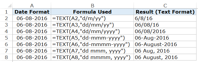
You can experiment with other formats as well and create your own combinations.

Also read: How to Convert Text to Date in Excel (8 Easy Ways)

Example 2: Converting Current Date to Text

To convert the current date into text, you can use the TODAY function along with the TEXT function.

Here is a formula that will do it:

="Today is "&TEXT(TODAY(),"dd/mm/yyyy")

This could be useful in dashboards/reports, where as soon as the file is opened (or any changes are made), the date refreshes to show the current date.

Convert Date to Text using Text to Column

If you’re not a fan of Excel formulas, there is another cool way to quickly convert date to text in Excel – the Text to Column feature.

Suppose you have a dataset as shown below and you want to convert these dates into text format:

Here are the steps to do this:

Select all the cells that contain dates that you want to convert to text.
Go to Data –> Data Tools –> Text to Column.
In the Text to Column Wizard, make the following selections:

This would instantly convert the dates into text format.

Note: There is a difference in the format of the dates in the two columns. While the original format had dd mmm, yyyy format, the result is dd-mm-yyyy. Remember that the Text to Column feature will always convert dates to the default short date format (which is dd-mm-yyyy as per my systems regional settings. It could be different for yours).

Also read: How to Convert Serial Numbers to Dates in Excel (2 Easy Ways)

If you want the date in other formats, use the formula method, or the copy-paste method shown below.

Convert Date to Text using the Copy-Paste Method

This is the fastest way to convert date to text.

Here are the steps:

You May Also Like the Following Excel Tutorials:

Convert Text to Numbers in Excel – A Step By Step Tutorial.
How to Convert Formulas to Values in Excel.
How to Quickly Transpose Data in Excel.
[Quick Tip] How to Split Cells in Excel.
Excel Timesheet Calculator Template.
How to Insert Date and Timestamp in Excel.
Excel Calendar Template.
How to Remove Time from Date in Excel
Convert Time to Decimal Number in Excel (Hours, Minutes, Seconds)
How To Convert Date To Serial Number In Excel?

Источник

In this example, the goal is to get the day name (i.e. Monday, Tuesday, Wednesday, etc.) from a given date. There are several ways to go about this in Excel, depending on your needs. This article explains three approaches:

Display date with a custom number format
Convert date to day name with TEXT function
Convert date to day name with CHOOSE function

For all examples, keep in mind that Excel dates are large serial numbers, displayed as dates with number formatting.

Day name with custom number format

To display a date using only the day name, you don’t need a formula; you can just use a custom number format. Select the date, and use the shortcut Control + 1 to open Format cells. Then select Number > Custom, and enter one of these custom formats:

"ddd"  // i.e."Wed"
"dddd" // i.e."Wednesday"

Excel will display only the day name, but it will leave the date intact. If you want to display both the date and the day name in different columns, one option is to use a formula to pick up a date from another cell, and change the number format to show only the day name. For example, in the worksheet shown, cell F5 contains the date January 1, 2000. The formula in G5, copied down, is:

=F5 // get date from F5

Cells G5 and G6 have the number format «dddd» applied, and cells in G7:G9 have the number format «ddd» applied.

Day name with TEXT function

To convert a date to a text value like «Saturday», you can use the TEXT function. The TEXT function is a general function that can be used to convert numbers of all kinds into text values with formatting, including date formats. For example, with the date January 1, 2000 in cell A1, you can use TEXT like this:

=TEXT(A1,"d-mmm-yyyy") // returns "1-Jan-2000"
=TEXT(A1,"mmmm d, yyyy") // returns "January 1, 2000"
=TEXT(A1,"mmmm") // returns "January"

In the worksheet shown, the goal is to display the day name only, so we use a custom number format like «ddd» or «dddd»:

=TEXT(B5,"dddd") // returns "Saturday"
=TEXT(B5,"ddd") // returns "Sat"

Note: The TEXT function converts a date to a text value using the supplied number format. The date is lost in the conversion and only the text for the day name remains.

Day name with CHOOSE function

For maximum flexibility, you can create your own day names with the CHOOSE function. CHOOSE is a general-purpose function for returning a value based on a numeric index. For example, you can use CHOOSE to return one of three colors with a number like this:

=CHOOSE(1,"red","blue","green") // returns "red"
=CHOOSE(2,"red","blue","green") // returns "blue"
=CHOOSE(3,"red","blue","green") // returns "green"

In this example, the goal is to return a day name from a date, so we need to configure CHOOSE to select one of seven-day names. For example, the formula below would return «Wed» based on a numeric index of 4:

=CHOOSE(4,"Sun","Mon","Tue","Wed","Thu","Fri","Sat") // "Wed"

The challenge in this case is to get the right index for a date and for that we need the WEEKDAY function. For any given date, WEEKDAY returns a number between 1-7, which corresponds to the day of the week. By default, WEEKDAY returns 1 for Sunday, 2 for Monday, 3 for Tuesday, etc. In the worksheet shown, the formula in C12 is:

=CHOOSE(WEEKDAY(B12),"Sun","Mon","Tue","Wed","Thu","Fri","Sat")

WEEKDAY returns a number between 1-7, and CHOOSE will use this number to select the corresponding value in the list. Since the date in B12 is January 1, 2000, WEEKDAY returns 7, and CHOOSE returns «Sat».

CHOOSE is more work to set up, but it is also more flexible, since it allows you to convert a date to a day name using any values you want. For example, you can use custom abbreviations or even abbreviations in a different language. In cell C15, CHOOSE is set up to use one letter abbreviations that correspond to Spanish day names:

=CHOOSE(WEEKDAY(B15),"D","L","M","X","J","V","S")

Empty cells

If you use the formulas above on an empty cell, you’ll get «Saturday» as the result. This happens because an empty cell is evaluated as zero, and zero in the Excel date system is the date «0-Jan-1900», which is a Saturday. To work around this issue, you can use the IF function to return an empty string («») for empty cells. For example, if cell A1 may or may not contain a date, you can use IF like this:

=IF(A1<>"",TEXT(A1,"ddd"),"") // check for empty cells

The literal translation of this formula is: If A1 is not empty, return the TEXT formula, otherwise return an empty string («»).

Источник