
Data Filter in Excel (Table of Contents)
- Data Filter in Excel
- Uses of Data Filter in Excel
- Types of Data Filter in Excel
- How to Add Data Filter in Excel?
Data Filter in Excel
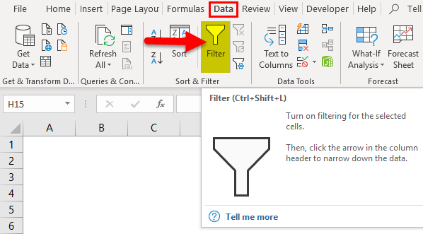
Data Filter in excel has many purposes apart from filtering the data. Although its main purpose is to filter the data as per the required condition, apart from this, we can sort, arrange the data, filter the data as per the color of cells or fonts or any condition available in the Text filter in the column where the filter is applied. To apply the filter, first, select the row where we need a filter, then from the Data menu tab, select Filter from Sort & Filter section. Or else we can apply filter by using short cut key ALT + D + F + F simultaneously or Ctrl + Shift + L together.
Uses of Data Filter in Excel
- If the table or range contains a huge number of datasets, it’s very difficult to find & extract the precise requested information or data. In this scenario, the Data Filter helps out.
- Data Filter in Excel option helps out in many ways to filter the data based on text, value, numeric or date value.
- The Data Filter option is very helpful to sort out data with simple drop-down menus.
- The Data Filter option is significant to temporarily hide few data sets in a table so that you can focus on the relevant data we need to work on.
- Filters are applied to rows of data in the worksheet.
- Apart from multiple filtering options, auto-filter criteria provide the Sort options also relevant to a given column.
Definition
Data Filter in Excel: it’s a quick way to display only the relevant or specific information which we need & temporarily hide irrelevant information or data in a table.
To activate the Excel data filter for any data in excel, select the entire data range or table range and click on the Filter button in the Data tab in the Excel ribbon.
(keyboard shortcut – Control + Shift + L)
Types of Data Filter in Excel
There are three types of data filtering options:
1. Data Filter Based On Text Values – It is used when the cells contain TEXT values; it has below mentioned Filtering Operators (Explained in example 1).
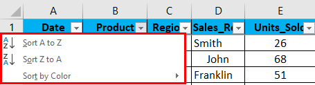
Apart from multiple filtering options in a text value, AutoFilter criteria provide the Sort options also relevant to a given column. i.e. Sort by A to Z, Sort by Z to A, and Sort by Color.
2. Data Filter Based on Numeric Values – It is used when the cells contain numbers or numeric values
It has below mentioned Filtering Operators (Explained in example 2)
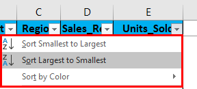
Apart from multiple filtering options in Numeric value, AutoFilter criteria provide the Sort options also relevant to a given column. i.e. Sort by Smallest to Largest, Sort by Largest to Smallest, and Sort by Color.
3. Data Filter Based On Date Values – It is used when the cells contain date values (Explained in example 3)
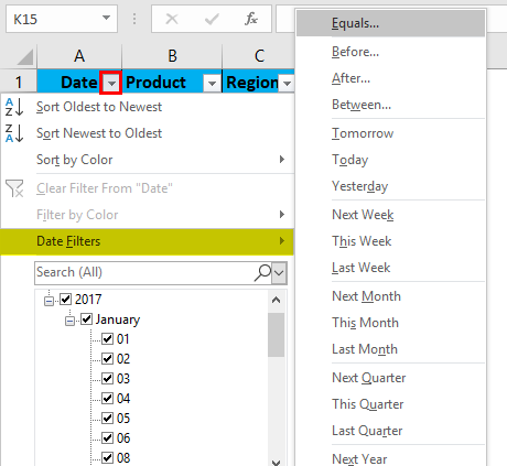
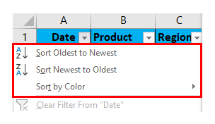
Apart from multiple filtering options in date value, AutoFilter criteria provide the Sort options also relevant to a given column. i.e. Sort by Oldest to Newest, Sort by Newest to Oldest, and Sort by Color.
How to Add Data Filter in Excel?
This Data Filter is very simple easy to use. Let us now see how to Add a Data Filter in Excel with the help of some examples.
You can download this Data Filter Excel Template here – Data Filter Excel Template
Example #1 – Filtering Based on Text Values or Data
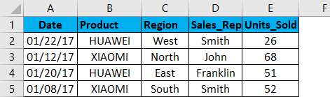
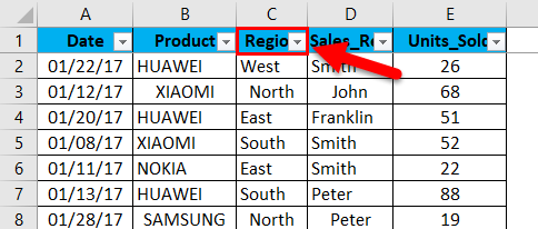
In the below-mentioned example, the Mobile sales data table contains a huge list of datasets.
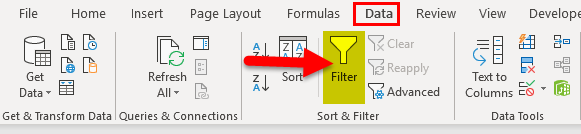
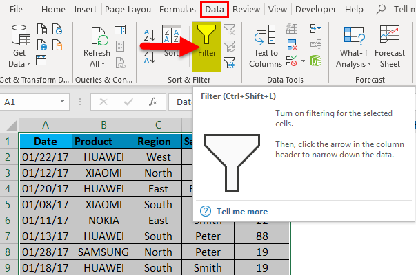
Initially, I have to activate the Excel data filter for the Mobile sales data table in excel, select the entire data range or table range, and click on the Filter button in the Data tab in the Excel ribbon.
Or click (keyboard shortcut – Control + Shift + L)
When you click on Filter, each column in the first row will automatically have a small drop-down button or filter icon added at the right corner of the cell i.e.
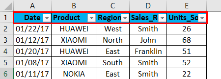
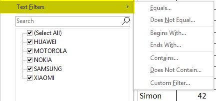
When excel identifies that the column contains text data, it automatically displays the option of text filters. In the mobile sales data, if I want sales data in the northern region only, irrespective of date, product, sales rep & units sold. I need to select the filter icon in the region header; I have to uncheck or deselect all the regions except the north region. It returns mobile sales data in the northern region only.
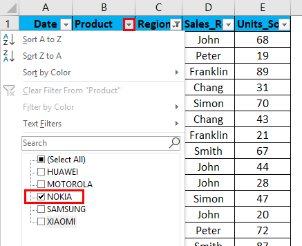
Once a filter is applied in the region column, Excel pinpoints you that table is filtered on a particular column by adding a funnel icon to the region column’s drop-down list button.
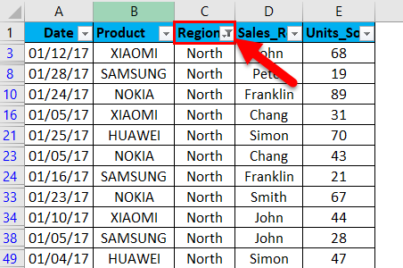
I can further filter based on brand & sales rep data. Now with this data, I further filter in the product region where I want the sales of the Nokia brand in the north region only irrespective of the sales rep, units sold & date.
I have to just apply the filter in the product column apart from the region column. I have to uncheck or deselect all the products except the NOKIA brand. It returns Nokia sales data in the north region.
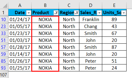
Once the filter is applied in the product column, Excel pinpoints you that table is filtered on a particular column by adding a funnel icon to the product column’s drop-down list button.
Example #2 – Filtering Based on Numeric Values or Data
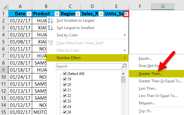
When excel identifies that the column contains NUMERIC values or data, it automatically displays the option of text filters.
If I want data of units sold in the mobile sales data, which is more than 30 units, irrespective of date, product, sales rep & region. For that, I need to select the filter icon in the units sold header; I have to select the number of filters, and under that greater than an option.
Once greater than option under number filter is selected, pop up appears, i.e. Custom auto filter, in that under the unit sold, we want datasets of more than 30 units sold, so enter 30. Click ok.
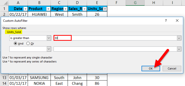
It returns mobile sales data based on the units sold. i.e. more than 30 units only.
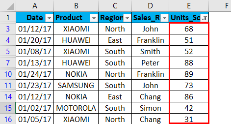
Once the filter is applied in the units sold column, Excel pinpoints you that table is filtered on a particular column by adding a funnel icon to the units sold column drop-down list button.
Sales data can be further Sorted by Smallest to Largest or Largest to Smallest in units sold.
Example #3 – Filtering based on Date Value
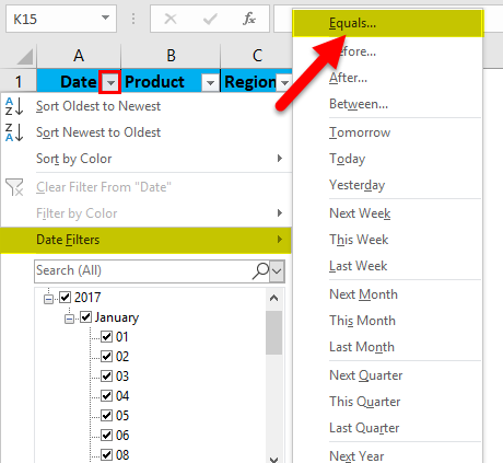
When excel identifies that the column contains DATE values or data, it automatically displays the option of DATE filters.
Date filter lets you filter dates based on any date range. For example, you can filter on conditions such dates by day, week, month, year, quarter, or year-to-date.
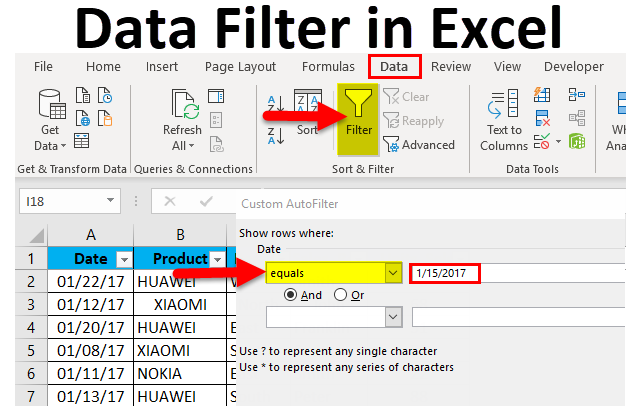
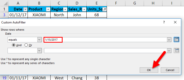
In the mobile sales data, if I want mobile sales data only on or for the date value, i.e. 01/15/17, irrespective of units sold, product, sales rep & region. I need to select the filter icon in the date header; I have to select the date filter, and under that equals to option.
Custom AutoFilter dialog box will appear; enter a date value manually, i.e. 01/15/17
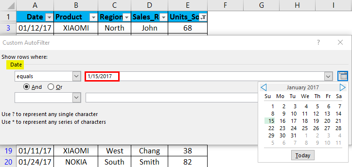
Click ok. It returns mobile sales data only on or for the date value, i.e. 01/15/17
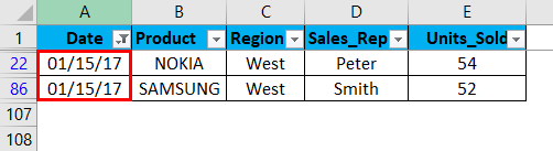
Once a filter is applied in the date column, Excel pinpoints you that table is filtered on a particular column by adding a funnel icon to the date column drop-down list button.
Things to Remember
- Data filter helps out to specify the required data that you want to display. This process is also called “Grouping of data, ” which helps out better analyse your data.
- Excel data can also be used to search or filter a data set with a specific word in a text with the help of a custom auto filter on the condition it contains ‘a’ or any relevant word of your choice.
- Data Filter option can be removed with the below-mentioned steps:
Go to the Data tab > Sort & Filter group and click Clear.
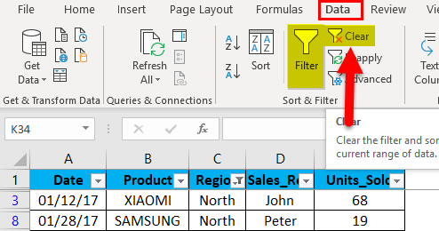
A Data Filter option is Removed.
- Excel data filter option can filter the records by multiple criteria or conditions, i.e. by filtering multiple column values (more than one column) explained in example 1.
- Excel data filter helps out to sort out blank & non-blank cells in the column.
- Data can also be filtered out with the help of wild characters, i.e.? (question mark) & * (asterisk) & ~ (tilde)
Recommended Articles
This has been a guide to a Data Filter in Excel. Here we discuss how to Add a Data Filter in Excel with excel examples and downloadable excel templates. You may also look at these useful functions in Excel –
- Excel Filter Shortcuts
- Excel Column Filter
- Advanced Filter in Excel
- VBA Filter
Use AutoFilter or built-in comparison operators like «greater than» and “top 10” in Excel to show the data you want and hide the rest. Once you filter data in a range of cells or table, you can either reapply a filter to get up-to-date results, or clear a filter to redisplay all of the data.
Use filters to temporarily hide some of the data in a table, so you can focus on the data you want to see.

Filter a range of data
-
Select any cell within the range.
-
Select Data > Filter.

-
Select the column header arrow
. -
Select Text Filters or Number Filters, and then select a comparison, like Between.
-
Enter the filter criteria and select OK.

 .
.

Filter data in a table
When you put your data in a table, filter controls are automatically added to the table headers.

-
Select the column header arrow
for the column you want to filter. -
Uncheck (Select All) and select the boxes you want to show.
-
Click OK.
The column header arrow
changes to a Filter icon. Select this icon to change or clear the filter.
 for the column you want to filter.
 Filter icon. Select this icon to change or clear the filter.
Related Topics
Excel Training: Filter data in a table
Guidelines and examples for sorting and filtering data by color
Filter data in a PivotTable
Filter by using advanced criteria
Remove a filter
Filtered data displays only the rows that meet criteria that you specify and hides rows that you do not want displayed. After you filter data, you can copy, find, edit, format, chart, and print the subset of filtered data without rearranging or moving it.
You can also filter by more than one column. Filters are additive, which means that each additional filter is based on the current filter and further reduces the subset of data.
Note: When you use the Find dialog box to search filtered data, only the data that is displayed is searched; data that is not displayed is not searched. To search all the data, clear all filters.
The two types of filters
Using AutoFilter, you can create two types of filters: by a list value or by criteria. Each of these filter types is mutually exclusive for each range of cells or column table. For example, you can filter by a list of numbers, or a criteria, but not by both; you can filter by icon or by a custom filter, but not by both.
Reapplying a filter
To determine if a filter is applied, note the icon in the column heading:
-
A drop-down arrow
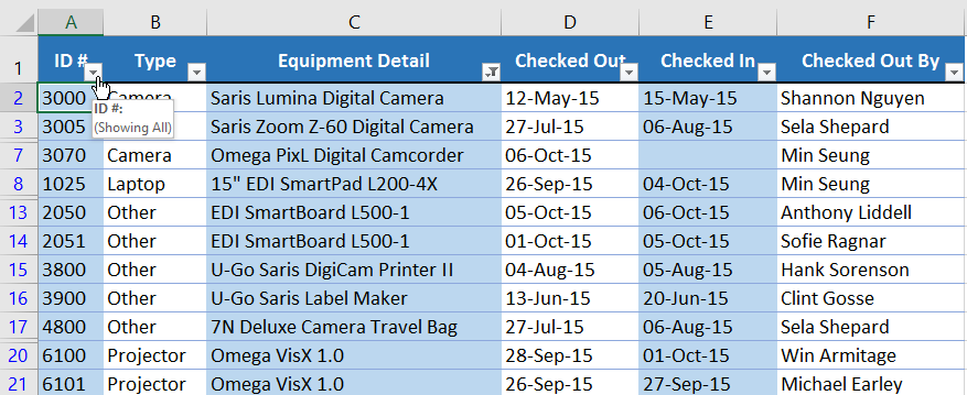
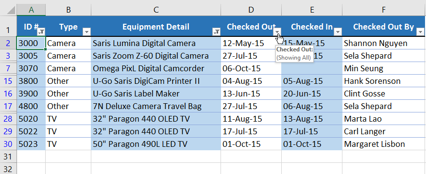
means that filtering is enabled but not applied.When you hover over the heading of a column with filtering enabled but not applied, a screen tip displays «(Showing All)».
-
A Filter button
means that a filter is applied.When you hover over the heading of a filtered column, a screen tip displays the filter applied to that column, such as «Equals a red cell color» or «Larger than 150».
When you reapply a filter, different results appear for the following reasons:
-
Data has been added, modified, or deleted to the range of cells or table column.
-
Values returned by a formula have changed and the worksheet has been recalculated.
Do not mix data types
For best results, do not mix data types, such as text and number, or number and date in the same column, because only one type of filter command is available for each column. If there is a mix of data types, the command that is displayed is the data type that occurs the most. For example, if the column contains three values stored as number and four as text, the Text Filters command is displayed .
Filter data in a table
When you put your data in a table, filtering controls are added to the table headers automatically.
-
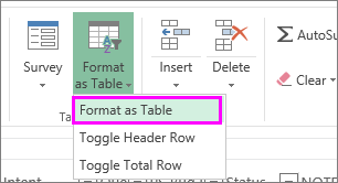
Select the data you want to filter. On the Home tab, click Format as Table, and then pick Format as Table.
-
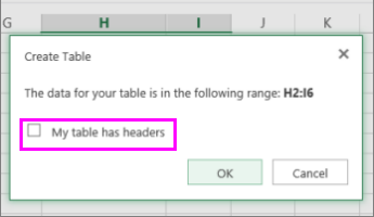
In the Create Table dialog box, you can choose whether your table has headers.
-
Select My table has headers to turn the top row of your data into table headers. The data in this row won’t be filtered.
-
Don’t select the check box if you want Excel for the web to add placeholder headers (that you can rename) above your table data.
-
-
Click OK.
-
To apply a filter, click the arrow in the column header, and pick a filter option.
Filter a range of data
If you don’t want to format your data as a table, you can also apply filters to a range of data.
-
Select the data you want to filter. For best results, the columns should have headings.
-
On the Data tab, choose Filter.
Filtering options for tables or ranges
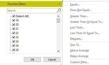
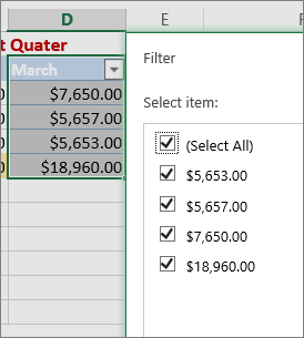
You can either apply a general Filter option or a custom filter specific to the data type. For example, when filtering numbers, you’ll see Number Filters, for dates you’ll see Date Filters, and for text you’ll see Text Filters. The general filter option lets you select the data you want to see from a list of existing data like this:
Number Filters lets you apply a custom filter:
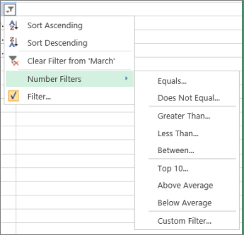
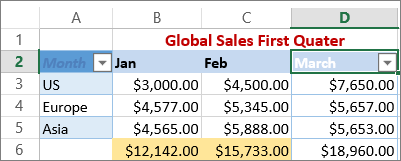
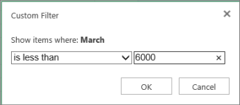
In this example, if you want to see the regions that had sales below $6,000 in March, you can apply a custom filter:
Here’s how:
-
Click the filter arrow next to March > Number Filters > Less Than and enter 6000.
-
Click OK.
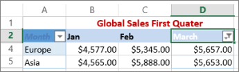
Excel for the web applies the filter and shows only the regions with sales below $6000.
You can apply custom Date Filters and Text Filters in a similar manner.
To clear a filter from a column
-
Click the Filter
button next to the column heading, and then click Clear Filter from <«Column Name»>.
To remove all the filters from a table or range
-
Select any cell inside your table or range and, on the Data tab, click the Filter button.
This will remove the filters from all the columns in your table or range and show all your data.
-
Click a cell in the range or table that you want to filter.
-
On the Data tab, click Filter.
-
Click the arrow
in the column that contains the content that you want to filter. -
Under Filter, click Choose One, and then enter your filter criteria.

 in the column that contains the content that you want to filter.
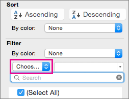
Notes:
-
You can apply filters to only one range of cells on a sheet at a time.
-
When you apply a filter to a column, the only filters available for other columns are the values visible in the currently filtered range.
-
Only the first 10,000 unique entries in a list appear in the filter window.
-
Click a cell in the range or table that you want to filter.
-
On the Data tab, click Filter.
-
Click the arrow
in the column that contains the content that you want to filter. -
Under Filter, click Choose One, and then enter your filter criteria.
-
In the box next to the pop-up menu, enter the number that you want to use.
-
Depending on your choice, you may be offered additional criteria to select:
Notes:
-
You can apply filters to only one range of cells on a sheet at a time.
-
When you apply a filter to a column, the only filters available for other columns are the values visible in the currently filtered range.
-
Only the first 10,000 unique entries in a list appear in the filter window.
-
Instead of filtering, you can use conditional formatting to make the top or bottom numbers stand out clearly in your data.
You can quickly filter data based on visual criteria, such as font color, cell color, or icon sets. And you can filter whether you have formatted cells, applied cell styles, or used conditional formatting.
-
In a range of cells or a table column, click a cell that contains the cell color, font color, or icon that you want to filter by.
-
On the Data tab, click Filter .
-
Click the arrow
in the column that contains the content that you want to filter. -
Under Filter, in the By color pop-up menu, select Cell Color, Font Color, or Cell Icon, and then click a color.
 in the column that contains the content that you want to filter.
This option is available only if the column that you want to filter contains a blank cell.
-
Click a cell in the range or table that you want to filter.
-
On the Data toolbar, click Filter.
-
Click the arrow
in the column that contains the content that you want to filter. -
In the (Select All) area, scroll down and select the (Blanks) check box.
Notes:
-
You can apply filters to only one range of cells on a sheet at a time.
-
When you apply a filter to a column, the only filters available for other columns are the values visible in the currently filtered range.
-
Only the first 10,000 unique entries in a list appear in the filter window.
-
-
Click a cell in the range or table that you want to filter.
-
On the Data tab, click Filter .
-
Click the arrow
in the column that contains the content that you want to filter. -
Under Filter, click Choose One, and then in the pop-up menu, do one of the following:
To filter the range for
Click
Rows that contain specific text
Contains or Equals.
Rows that do not contain specific text
Does Not Contain or Does Not Equal.
-
In the box next to the pop-up menu, enter the text that you want to use.
-
Depending on your choice, you may be offered additional criteria to select:
To
Click
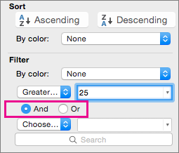
Filter the table column or selection so that both criteria must be true
And.
Filter the table column or selection so that either or both criteria can be true
Or.
-
Click a cell in the range or table that you want to filter.
-
On the Data toolbar, click Filter .
-
Click the arrow
in the column that contains the content that you want to filter. -
Under Filter, click Choose One, and then in the pop-up menu, do one of the following:
To filter for
Click
The beginning of a line of text
Begins With.
The end of a line of text
Ends With.
Cells that contain text but do not begin with letters
Does Not Begin With.
Cells that contain text but do not end with letters
Does Not End With.
-
In the box next to the pop-up menu, enter the text that you want to use.
-
Depending on your choice, you may be offered additional criteria to select:
To
Click
Filter the table column or selection so that both criteria must be true
And.
Filter the table column or selection so that either or both criteria can be true
Or.
Wildcard characters can be used to help you build criteria.
-
Click a cell in the range or table that you want to filter.
-
On the Data toolbar, click Filter.
-
Click the arrow
in the column that contains the content that you want to filter. -
Under Filter, click Choose One, and select any option.
-
In the text box, type your criteria and include a wildcard character.
For example, if you wanted your filter to catch both the word «seat» and «seam», type sea?.
-
Do one of the following:
Use
To find
? (question mark)
Any single character
For example, sm?th finds «smith» and «smyth»
* (asterisk)
Any number of characters
For example, *east finds «Northeast» and «Southeast»
~ (tilde)
A question mark or an asterisk
For example, there~? finds «there?»
Do any of the following:
|
To |
Do this |
|---|---|
|
Remove specific filter criteria for a filter |
Click the arrow |
|
Remove all filters that are applied to a range or table |
Select the columns of the range or table that have filters applied, and then on the Data tab, click Filter. |
|
Remove filter arrows from or reapply filter arrows to a range or table |
Select the columns of the range or table that have filters applied, and then on the Data tab, click Filter. |
When you filter data, only the data that meets your criteria appears. The data that doesn’t meet that criteria is hidden. After you filter data, you can copy, find, edit, format, chart, and print the subset of filtered data.
Table with Top 4 Items filter applied
Filters are additive. This means that each additional filter is based on the current filter and further reduces the subset of data. You can make complex filters by filtering on more than one value, more than one format, or more than one criteria. For example, you can filter on all numbers greater than 5 that are also below average. But some filters (top and bottom ten, above and below average) are based on the original range of cells. For example, when you filter the top ten values, you’ll see the top ten values of the whole list, not the top ten values of the subset of the last filter.
In Excel, you can create three kinds of filters: by values, by a format, or by criteria. But each of these filter types is mutually exclusive. For example, you can filter by cell color or by a list of numbers, but not by both. You can filter by icon or by a custom filter, but not by both.
Filters hide extraneous data. In this manner, you can concentrate on just what you want to see. In contrast, when you sort data, the data is rearranged into some order. For more information about sorting, see Sort a list of data.
When you filter, consider the following guidelines:
-
Only the first 10,000 unique entries in a list appear in the filter window.
-
You can filter by more than one column. When you apply a filter to a column, the only filters available for other columns are the values visible in the currently filtered range.
-
You can apply filters to only one range of cells on a sheet at a time.
Note: When you use Find to search filtered data, only the data that is displayed is searched; data that is not displayed is not searched. To search all the data, clear all filters.
Need more help?
You can always ask an expert in the Excel Tech Community or get support in the Answers community.
Wherever there is data, there is a need to filter it.
Excel Data Filter feature gives you many ways to filter the data – based on text, value or date.
Excel Data Filter
Suppose you have the data as shown below:

To activate Excel data filter for this data, select the entire data and click on the Filter button in the Data tab in Excel ribbon (keyboard shortcut – Control + Shift + L)

Once you apply filter to the data, you will see a filter icon in each of the header cells of your data ![]()
When you click on this filter icon, you can access all the filter and sorting options available for that column of the data. There are three kinds of data filtering that can be applied:
- Based in Text Data
- Based on Numbers
- Based on Dates
Filtering based on Text Data
This kind of filter would be applicable for the first two columns of this data set (Sales Rep Name and Quarter), as it has text data in it. Once you have applied the filter, click on the filter icon at the right of the header cell.
When you click on the filter icon, it displays the drop down as shown below:

Since Excel has identified that the column has text data, it automatically displays the option for text filters. You can either type the text in the Search bar, check/un-check names, or use the in-built text filter conditions.
Suppose you want to filter all the Sales Rep Names whose name begin with the alphabet “A”. To do this, select the Begins With condition in Text Filter conditions:

Filtering based on Numbers
This filter can be applied on the last column in out data set (for sales values). Once you have applied the filter, click on the filter icon at the right of the header cell.
When you click on the filter icon, it displays the drop down as shown below:
 Since Excel has identified that the column has numbers, it automatically displays the option for Number filters. You can either type the number in the Search bar, check/un-check number values, or use the in-built text filter conditions.
Suppose you want to filter all the sales value above 3000. To do this, select the Greater than option from the Number Filters list

Filtering Based on Dates
This filter can be applied on the second last column in out data set (for date). Once you have applied the filter, click on the filter icon at the right of the header cell.
When you click on the filter icon, it displays the drop down as shown below:
 Date filter lets you filter dates based on current date. For example, you can filter on conditions such as today, tomorrow, or yesterday. Similarly, you can can filter on current/next/previous month, quarter, or year.
To remove filters from your data set, go to data tab and again click on the filter icon (or use keyboard shortcut – Control + Shift + L).
Note:
- Excel determines which type of filter to apply based in the data set. If there are more text values than numbers, then text filter is applied, else number filter is applied.
- In case you need more functionality in filtering data, use Exel Advanced Filter.
- Apart from filtering, you can also access all the sorting criteria after applying filter (Learn all about data sorting in Excel).
Related Tutorials on Data Filtering:
- Filter Cells with Bold Font Formatting.
- Dynamic Excel Filter – Filters Data as you Type.
- Filter By Color in Excel
Often you may want to filter dates by month in Excel.
Fortunately this is easy to do using the Filter function.
The following step-by-step example shows how to use this function to filter dates by month in Excel.
Step 1: Create the Data
First, let’s create a dataset that shows the total sales made by some company on various days:

Step 2: Add a Filter
Next, highlight the cells in the range A1:B13 and then click the Data tab along the top ribbon and click the Filter button:

A dropdown filter will automatically be added to the first row of column A and column B.
Step 3: Filter Dates by Month
Next, we’ll filter the data to only show the rows where the month contains February.
Click the dropdown arrow next to Date, then uncheck all of the boxes except the one next to February and then click OK:

The data will automatically be filtered to only show the rows where the date is in February:

Note that if you have multiple years and you’d like to filter the data to only show the dates in February (while ignoring year), you can click the dropdown arrow next to Date, then Date Filters, then All Dates in the Period, then February:

The data will automatically be filtered to only show the rows where the date is in February, regardless of the year.
Additional Resources
The following tutorials explain how to perform other common operations in Excel:
How to Group Data by Month in Excel
How to AutoFill Dates in Excel
How to Calculate the Difference Between Two Dates in Excel
Lesson 20: Filtering Data
/en/excel/sorting-data/content/
Introduction
If your worksheet contains a lot of content, it can be difficult to find information quickly. Filters can be used to narrow down the data in your worksheet, allowing you to view only the information you need.
Optional: Download our practice workbook.
Watch the video below to learn more about filtering data in Excel.
To filter data:
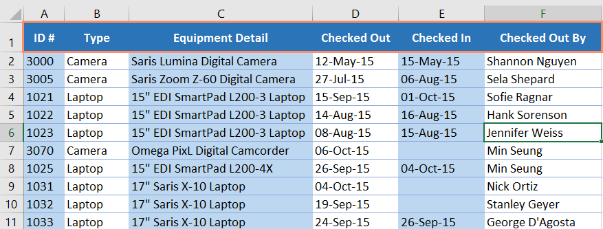
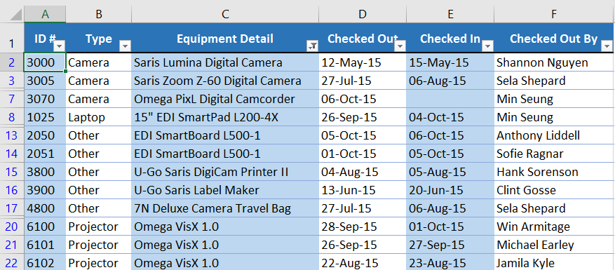
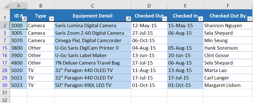
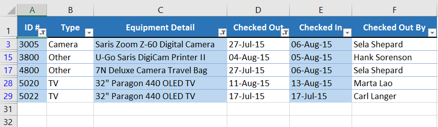
In our example, we’ll apply a filter to an equipment log worksheet to display only the laptops and projectors that are available for checkout.
- In order for filtering to work correctly, your worksheet should include a header row, which is used to identify the name of each column. In our example, our worksheet is organized into different columns identified by the header cells in row 1: ID#, Type, Equipment Detail, and so on.

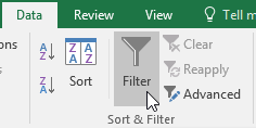
- Select the Data tab, then click the Filter command.
- A drop-down arrow will appear in the header cell for each column.
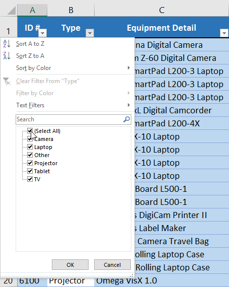
- Click the drop-down arrow for the column you want to filter. In our example, we will filter column B to view only certain types of equipment.
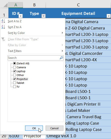
- The Filter menu will appear.
- Uncheck the box next to Select All to quickly deselect all data.
- Check the boxes next to the data you want to filter, then click OK. In this example, we will check Laptop and Projector to view only these types of equipment.
- The data will be filtered, temporarily hiding any content that doesn’t match the criteria. In our example, only laptops and projectors are visible.

Filtering options can also be accessed from the Sort & Filter command on the Home tab.

To apply multiple filters:
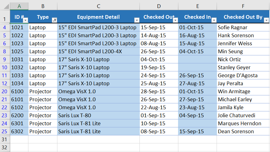
Filters are cumulative, which means you can apply multiple filters to help narrow down your results. In this example, we’ve already filtered our worksheet to show laptops and projectors, and we’d like to narrow it down further to only show laptops and projectors that were checked out in August.
- Click the drop-down arrow for the column you want to filter. In this example, we will add a filter to column D to view information by date.

- The Filter menu will appear.
- Check or uncheck the boxes depending on the data you want to filter, then click OK. In our example, we’ll uncheck everything except for August.
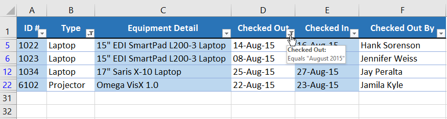
- The new filter will be applied. In our example, the worksheet is now filtered to show only laptops and projectors that were checked out in August.

To clear a filter:
After applying a filter, you may want to remove—or clear—it from your worksheet so you’ll be able to filter content in different ways.
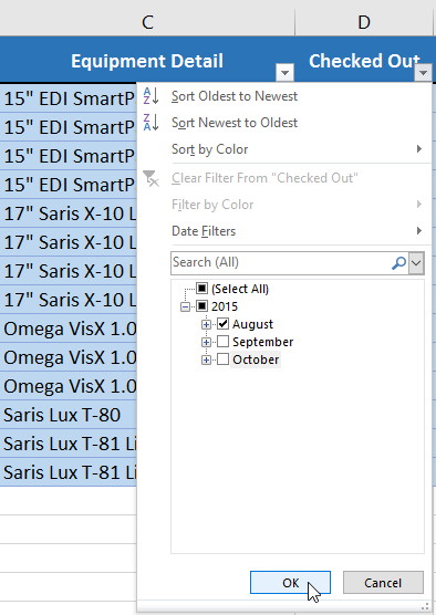
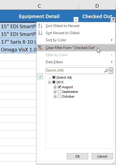
- Click the drop-down arrow for the filter you want to clear. In our example, we’ll clear the filter in column D.
- The Filter menu will appear.
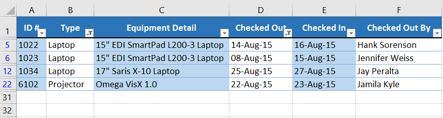
- Choose Clear Filter From [COLUMN NAME] from the Filter menu. In our example, we’ll select Clear Filter From «Checked Out«.
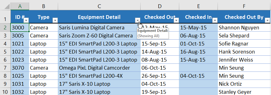
- The filter will be cleared from the column. The previously hidden data will be displayed.
To remove all filters from your worksheet, click the Filter command on the Data tab.
Advanced filtering
If you need a filter for something specific, basic filtering may not give you enough options. Fortunately, Excel includes several advanced filtering tools, including search, text, date, and number filtering, which can narrow your results to help find exactly what you need.
To filter with search:
Excel allows you to search for data that contains an exact phrase, number, date, and more. In our example, we’ll use this feature to show only Saris brand products in our equipment log.
- Select the Data tab, then click the Filter command. A drop-down arrow will appear in the header cell for each column. Note: If you’ve already added filters to your worksheet, you can skip this step.
- Click the drop-down arrow for the column you want to filter. In our example, we’ll filter column C.

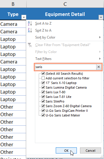
- The Filter menu will appear. Enter a search term into the search box. Search results will appear automatically below the Text Filters field as you type. In our example, we’ll type saris to find all Saris brand equipment. When you’re done, click OK.
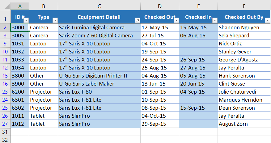
- The worksheet will be filtered according to your search term. In our example, the worksheet is now filtered to show only Saris brand equipment.

To use advanced text filters:
Advanced text filters can be used to display more specific information, like cells that contain a certain number of characters or data that excludes a specific word or number. In our example, we’d like to exclude any item containing the word laptop.
- Select the Data tab, then click the Filter command. A drop-down arrow will appear in the header cell for each column. Note: If you’ve already added filters to your worksheet, you can skip this step.
- Click the drop-down arrow for the column you want to filter. In our example, we’ll filter column C.
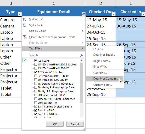
- The Filter menu will appear. Hover the mouse over Text Filters, then select the desired text filter from the drop-down menu. In our example, we’ll choose Does Not Contain… to view data that does not contain specific text.
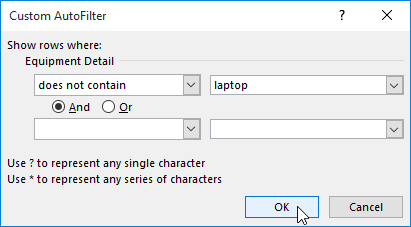
- The Custom AutoFilter dialog box will appear. Enter the desired text to the right of the filter, then click OK. In our example, we’ll type laptop to exclude any items containing this word.
- The data will be filtered by the selected text filter. In our example, our worksheet now displays items that do not contain the word laptop.

To use advanced number filters:
Advanced number filters allow you to manipulate numbered data in different ways. In this example, we’ll display only certain types of equipment based on the range of ID numbers.
- Select the Data tab on the Ribbon, then click the Filter command. A drop-down arrow will appear in the header cell for each column. Note: If you’ve already added filters to your worksheet, you can skip this step.
- Click the drop-down arrow for the column you want to filter. In our example, we’ll filter column A to view only a certain range of ID numbers.

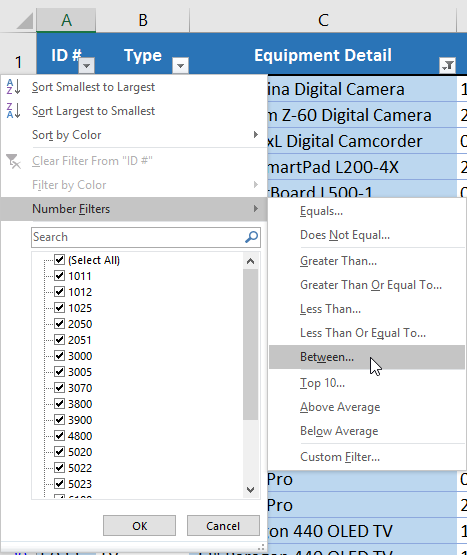
- The Filter menu will appear. Hover the mouse over Number Filters, then select the desired number filter from the drop-down menu. In our example, we’ll choose Between to view ID numbers between a specific number range.
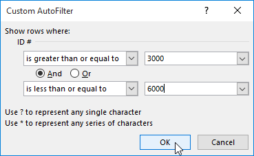
- The Custom AutoFilter dialog box will appear. Enter the desired number(s) to the right of each filter, then click OK. In our example, we want to filter for ID numbers greater than or equal to 3000 but less than or equal to 6000, which will display ID numbers in the 3000-6000 range.
- The data will be filtered by the selected number filter. In our example, only items with an ID number between 3000 and 6000 are visible.
To use advanced date filters:
Advanced date filters can be used to view information from a certain time period, such as last year, next quarter, or between two dates. In this example, we’ll use advanced date filters to view only equipment that has been checked out between July 15 and August 15.
- Select the Data tab, then click the Filter command. A drop-down arrow will appear in the header cell for each column. Note: If you’ve already added filters to your worksheet, you can skip this step.
- Click the drop-down arrow for the column you want to filter. In our example, we’ll filter column D to view only a certain range of dates.
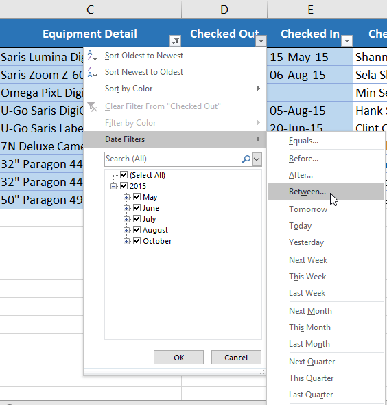
- The Filter menu will appear. Hover the mouse over Date Filters, then select the desired date filter from the drop-down menu. In our example, we’ll select Between… to view equipment that has been checked out between July 15 and August 15.
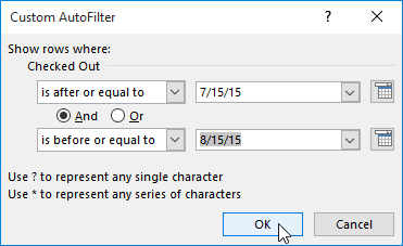
- The Custom AutoFilter dialog box will appear. Enter the desired date(s) to the right of each filter, then click OK. In our example, we want to filter for dates after or equal to July 15, 2015, and before or equal to August 15, 2015, which will display a range between these dates.
- The worksheet will be filtered by the selected date filter. In our example, we can now see which items have been checked out between July 15 and August 15.
Challenge!
- Open our practice workbook.
- Click the Challenge tab in the bottom-left of the workbook.
- Apply a filter to show only Electronics and Instruments.
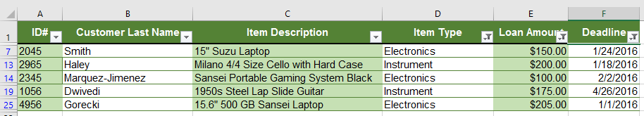
- Use the Search feature to filter item descriptions that contain the word Sansei. After you do this, you should have six entries showing.
- Clear the Item Description filter.
- Using a number filter, show loan amounts greater than or equal to $100.
- Filter to show only items that have deadlines in 2016.
- When you’re finished, your workbook should look like this:

/en/excel/groups-and-subtotals/content/
If you have a range of date, and if you want to filter the data as per year or month, you can do it by using the Format Cells and Auto filter option in Microsoft Excel.
In this article, we will learn using Format Cells to format the date in Month or Year as per the filtration requirement.
Let’s take an example to understand how we can filter the data by the date.
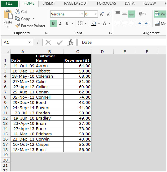
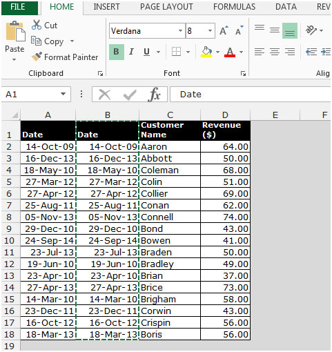
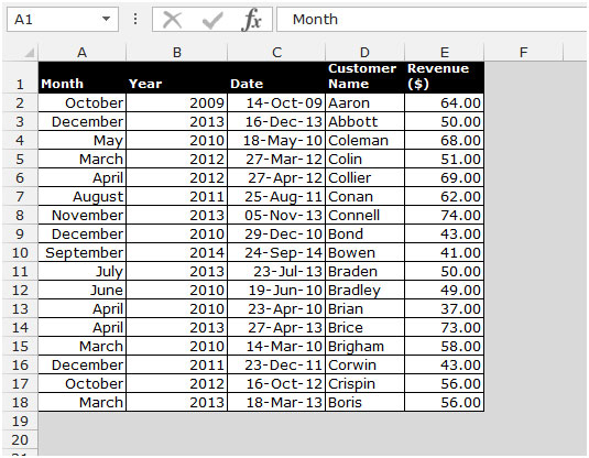
We have data in range A1: C18. Column A contains date, column B contains customer name and column C contains Revenue amount.
If we want to put the filter as per the Month and year, we need to follow below given steps:-
- Copy the range A1:A18 and paste it right side to Column A
- Select the date range A1:A18.
- Copy the date column by pressing the key Ctrl+C on your keyboard.

- Select the cell A1 and press the key Ctrl++.
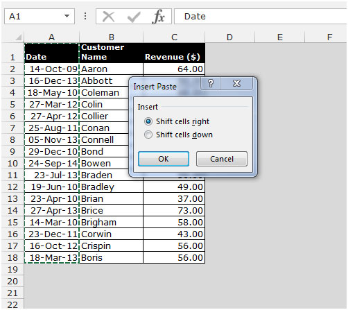
- Insert Paste dialog box will appear.
- Select Shift cells right and click on OK.
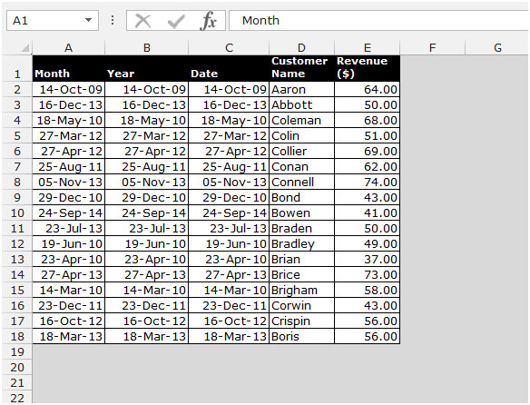
- Again, copy the range and press the Ctrl++, and select shift cells right in the insert paste dialog box and click on OK.

- Change the title for 2 columns to Month and year.
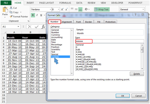
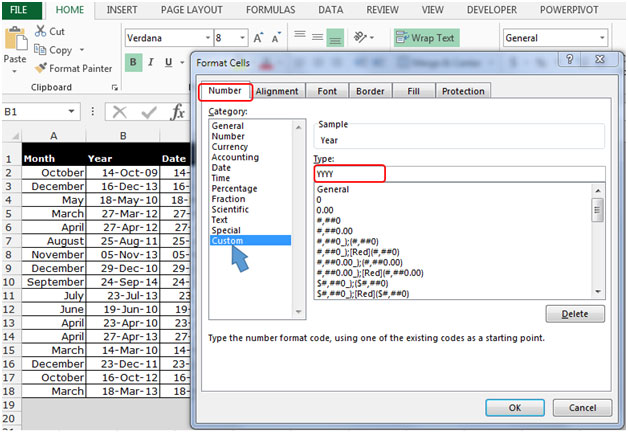
- Select the Month Column and press the Ctrl+1.
- Format cells dialog box will appear.
- Go to number tab and select custom.
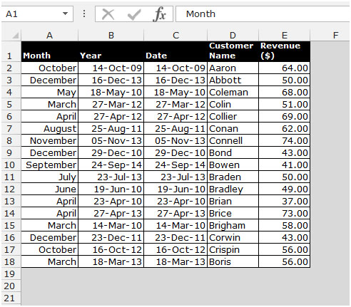
- In the type box, enter the format mmmm (to show the full name of month) and click on OK.
- Select the Year Column and press the Ctrl+1.
- Format cells dialog box will appear.
- Go to number tab and select custom.
- In the type box, enter the format YYYY (to show the full year) and click on OK.
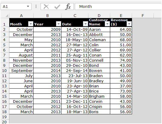
Now list is ready to filter the data according Month and year criteria.
- To insert the Auto Filter, select the cell A1 and press the key Ctrl+Shift+L.
To insert the Auto Filter, select the cell A1 and press the key Ctrl+Shift+L. And filter the data according to the month and year.
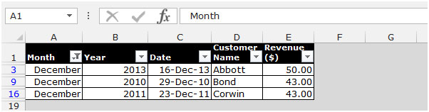

This is the way we can put the filter by the date field in Microsoft Excel.
На чтение 6 мин. Просмотров 7.9k.
Итог: узнайте, как применять фильтры даты с VBA. Включает примеры фильтрации для диапазона между двумя датами, группами дат из раскрывающегося списка фильтра, динамическими датами в периоде и т.д.
Уровень мастерства: Средний

Содержание
- Скачать файл
- Фильтры даты в Excel
- Фильтры диапазона дат в VBA
- Несколько групп дат
- Динамические даты в периодах
- Фильтры и типы данных
Скачать файл
Файл Excel, содержащий код, можно скачать ниже. Этот файл содержит код для фильтрации различных типов данных и типов фильтров. Пожалуйста, ознакомьтесь с моей статьей Фильтрация сводной таблицы или среза по самой последней дате или периоду для более подробной информации.
![]() VBA AutoFilters Guide.xlsm (100.5 KB)
VBA AutoFilters Guide.xlsm (100.5 KB)
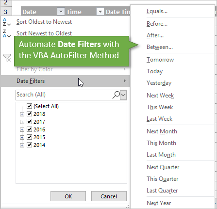
У нас есть много вариантов при фильтрации столбца, который
содержит даты. Список выпадающего меню фильтра группирует даты по годам,
месяцам, дням, часам, минутам, секундам. Мы можем расширить и установить эти
флажки для фильтрации нескольких элементов.
Мы также можем выбрать из подменю Date Filters. Это позволяет нам фильтровать диапазоны дат, как до, после или между двумя датами. Есть также много вариантов дат в периодах (этот месяц, следующий месяц, последний квартал и т.д.).
Давайте посмотрим на некоторые примеры кода для различных
фильтров даты.
При
применении фильтра для одного числа нам нужно использовать форматирование чисел,
которое применяется в столбце. Это странная причуда VBA, которая
может привести к неточным результатам, если вы не знаете правила. В приведенном
ниже коде есть пример.
Фильтры диапазона дат в VBA
Следующий макрос содержит примеры основных фильтров даты. Важно отметить, что значения параметров Criteria заключены в кавычки. Операторы сравнения = <> также включены в кавычки.
Пожалуйста, ознакомьтесь с моей статьей Фильтрация сводной таблицы или среза по самой последней дате или периоду для получения более подробной информации о том, как использовать метод AutoFilter и его параметры.
Вы можете скопировать / вставить приведенный ниже код в VB Editor.
Sub AutoFilter_Date_Examples()
' Примеры фильтрации столбцов с датами

Dim lo As ListObject
Dim iCol As Long

  ' Установить ссылку на первую таблицу на листе
  Set lo = Sheet1.ListObjects(1)

  ' Установить поле фильтра
  iCol = lo.ListColumns("Date").Index

  ' Очистить фильтры
  lo.AutoFilter.ShowAllData

  With lo.Range

    ' Одиночная дата - использовать тот же формат даты, который
     'применяется к столбцу
    .AutoFilter Field:=iCol, Criteria1:="=1/2/2014"

    'До даты
    .AutoFilter Field:=iCol, Criteria1:="<1/31/2014"

    'После или равно дате
    .AutoFilter Field:=iCol, Criteria1:=">=1/31/2014"

    'Диапазон дат (между датами)
    .AutoFilter Field:=iCol, _
                        Criteria1:=">=1/1/2014", _
                        Operator:=xlAnd, _
                        Criteria2:="<=12/31/2015"

End Sub
Несколько групп дат
Следующий макрос содержит примеры фильтрации нескольких
групп дат. Это то же самое, что выбрать конкретные годы, месяцы, дни, часы,
минуты из списка в раскрывающемся меню фильтра.
Для этих фильтров мы устанавливаем для параметра Operator
значение xlFilterValues. Мы используем Criteria2 (не Criteria1), чтобы указать
массив элементов с помощью функции Array.
Это специальный массив шаблонов, где первое число — это
период времени (год, месяцы, дни и т. Д.). Второе число — последняя дата в
диапазоне. Макрос ниже содержит примеры и дальнейшие пояснения.
Sub AutoFilter_Multiple_Dates_Examples()
'Примеры фильтрации столбцов для нескольких периодов времени даты

Dim lo As ListObject
Dim iCol As Long

  'Установить ссылку на первую таблицу на листе
  Set lo = Sheet1.ListObjects(1)

  'Установить поле фильтра
  iCol = lo.ListColumns("Date").Index

  'Очистить фильтры
  lo.AutoFilter.ShowAllData

  With lo.Range

    'При фильтрации по нескольким периодам, выбранным из
    'раскрывающегося меню фильтра, используйте Operator: = xlFilterValues и
    'Критерии2 с узорным массивом. Первое число -
    'временной период. Второе число - последняя дата в периоде.

    'Первое измерение массива - группа периода времени
      '0-Годы
      '1-Месяцы
      '2-Дни
      '3-Часы
      '4-Минуты
      '5-Секунды


    'Несколько лет (2014 и 2016) использовать последний день времени
    'периода для каждого элемента массива
    .AutoFilter Field:=iCol, _
                Operator:=xlFilterValues, _
                Criteria2:=Array(0, "12/31/2014", 0, "12/31/2016")

    'Несколько месяцев (январь, апрель, июль, октябрь 2015 года)
    .AutoFilter Field:=iCol, _
                Operator:=xlFilterValues, _
                Criteria2:=Array(1, "1/31/2015", 1, "4/30/2015", 1, "7/31/2015", 1, "10/31/2015")

    'Несколько дней
    'Последний день каждого месяца: январь, апрель, июль, октябрь 2015 года)
    .AutoFilter Field:=iCol, _
                Operator:=xlFilterValues, _
                Criteria2:=Array(2, "1/31/2015", 2, "4/30/2015", 2, "7/31/2015", 2, "10/31/2015")

    'Установить поле фильтра
     iCol = lo.ListColumns("Date Time").Index

    'Очистить фильтры
    lo.AutoFilter.ShowAllData

    'Несколько часов» (все даты в 11:00 часов 10 января 2008 г.
    'и 11:00 часов 20.01.2008)

    .AutoFilter Field:=iCol, _
                Operator:=xlFilterValues, _
                Criteria2:=Array(3, "1/10/2018 13:59:59", 3, "1/20/2018 23:59:59")

  End With

End Sub
Динамические даты в периодах
Следующий макрос содержит примеры дат в определенных
периодах. Это аналогично выбору предустановленных элементов фильтра из подменю «Фильтры
даты».
Для этих фильтров мы устанавливаем параметр Operator равным
xlFilterDynamic. Мы устанавливаем Criteria1 в константу, которая представляет
параметр периода динамической даты. Константы перечислены ниже.
Sub AutoFilter_Dates_in_Period_Examples()
'Примеры фильтрации столбцов для ДАТЫ В ПЕРИОД
'Пресеты фильтров даты, найденные в подменю «Фильтры даты

Dim lo As ListObject
Dim iCol As Long

  'Установить ссылку на первую таблицу на листе
  Set lo = Sheet1.ListObjects(1)

  'Установить поле фильтра
  iCol = lo.ListColumns("Date").Index

  'Очистить фильтры
  lo.AutoFilter.ShowAllData

  'Оператор: = xlFilterDynamic
  'Критерии1: = одно из следующих перечислений

  ' Значение константы
  ' 1     xlFilterToday
  ' 2     xlFilterYesterday
  ' 3     xlFilterTomorrow
  ' 4     xlFilterThisWeek
  ' 5     xlFilterLastWeek
  ' 6     xlFilterNextWeek
  ' 7     xlFilterThisMonth
  ' 8     xlFilterLastMonth
  ' 9     xlFilterNextMonth
  ' 10    xlFilterThisQuarter
  ' 11    xlFilterLastQuarter
  ' 12    xlFilterNextQuarter
  ' 13    xlFilterThisYear
  ' 14    xlFilterLastYear
  ' 15    xlFilterNextYear
  ' 16    xlFilterYearToDate
  ' 17    xlFilterAllDatesInPeriodQuarter1
  ' 18    xlFilterAllDatesInPeriodQuarter2
  ' 19    xlFilterAllDatesInPeriodQuarter3
  ' 20    xlFilterAllDatesInPeriodQuarter4
  ' 21    xlFilterAllDatesInPeriodJanuary
  ' 22    xlFilterAllDatesInPeriodFebruray <- февраль написан с ошибкой
  ' 23    xlFilterAllDatesInPeriodMarch
  ' 24    xlFilterAllDatesInPeriodApril
  ' 25    xlFilterAllDatesInPeriodMay
  ' 26    xlFilterAllDatesInPeriodJune
  ' 27    xlFilterAllDatesInPeriodJuly
  ' 28    xlFilterAllDatesInPeriodAugust
  ' 29    xlFilterAllDatesInPeriodSeptember
  ' 30    xlFilterAllDatesInPeriodOctober
  ' 31    xlFilterAllDatesInPeriodNovember
  ' 32    xlFilterAllDatesInPeriodDecember

  With lo.Range

    'Все даты в январе (по всем годам)
    .AutoFilter Field:=iCol, _
                Operator:=xlFilterDynamic, _
                Criteria1:=xlFilterAllDatesInPeriodJanuary

    'Все даты во втором квартале (по всем годам)
    .AutoFilter Field:=iCol, _
                Operator:=xlFilterDynamic, _
                Criteria1:=xlFilterAllDatesInPeriodQuarter2

  End With

End Sub
Вот ссылка на справочную страницу MSDN со списком XlDynamicFilterCriteria. И спасибо Дугу Глэнси из YourSumBuddy за то, что он указал на февральскую опечатку в константе. У него есть несколько полезных советов для параметра Operator в этой статье.
Фильтры и типы данных
Параметры
раскрывающегося меню фильтра изменяются в зависимости от типа данных в столбце.
У нас есть разные фильтры для текста, чисел, дат и цветов. Это создает МНОГО
различных комбинаций операторов и критериев для каждого типа фильтра.
Я создал отдельные статьи для каждого из этих типов фильтров. Статьи содержат пояснения и примеры кода VBA.
- Как очистить фильтры с помощью VBA
- Как отфильтровать пустые и непустые ячейки
- Как фильтровать числа с помощью VBA
- Как фильтровать текст с помощью VBA
- Как отфильтровать цвета и значки с помощью VBA
Файл в разделе загрузок выше содержит все эти примеры кода в одном месте. Вы можете добавить его в свою личную книгу макросов и использовать макросы в своих проектах.
Пожалуйста, оставьте
комментарий ниже с любыми вопросами или предложениями. Спасибо!
Summary
To filter data to include data based on dates, you can use the FILTER function with one of Excel’s date functions. In the example shown, the formula in F5 is:
=FILTER(data,MONTH(date)=7,"No data")
where data (B5:E15) and date (C5:C15) are named ranges. The result returned by FILTER includes data in the month of July only.
Generic formula
Explanation
This formula relies on the FILTER function to retrieve data based on a logical test created with the MONTH function. The array argument is provided as the named range data, which contains the full set of data without headers. The include argument is constructed with the MONTH function:
MONTH(date)=7
Here, MONTH receives the range C5:C15. Since the range contains 11 cells, MONTH returns an array with 11 results:
{6;7;7;7;7;8;8;8;8;8;8}
Each result is then compared to 7, and this operation creates an array of TRUE and FALSE values, which is delivered to the FILTER function as the include argument.
{FALSE;TRUE;TRUE;TRUE;TRUE;FALSE;FALSE;FALSE;FALSE;FALSE;FALSE}
Only rows where the result is TRUE make it into the final output. The if_empty argument is set to «No data» in case no matching data is found.
Filter by month and year
To filter by month and year, you can construct a formula using boolean logic like this:
=FILTER(data,(MONTH(date)=7)*(YEAR(date)=2019),"No data")
Although the values for month and year are hardcoded above into the formula, they can easily be replaced with cell references.

Author![]()
Dave Bruns
Hi — I’m Dave Bruns, and I run Exceljet with my wife, Lisa. Our goal is to help you work faster in Excel. We create short videos, and clear examples of formulas, functions, pivot tables, conditional formatting, and charts.
Bottom line: Learn how to apply date filters with VBA. Includes examples for filtering for a range between two dates, date groups from filter drop-down list, dynamic dates in period, etc.
Skill level: Intermediate
Download the File
The Excel file that contains the code can be downloaded below. This file contains code for filtering different data types and filter types. Please see my article on The Ultimate Guide to AutoFilters in VBA for more details.
Date Filters in Excel
We have a lot of options when filtering a column that contains dates. The filter drop-down menu list groups the dates by years, months, days, hours, minutes, seconds. We can expand and select those check boxes to filter multiple items.
We can also choose from the Date Filters sub menus. This allows us to filter for date ranges like before, after, or between two dates. There are also many options for dates in periods (This Month, Next Month, Last Quarter, etc.).
Let’s take a look at some code examples for the different date filters.
When applying a filter for a single number we need to use the number formatting that is applied in the column. This is a weird quirk of VBA that can cause inaccurate results if you don’t know the rule. There is an example in the code below.
Date Range Filters in VBA
The following macro contains examples for basic date filters. It’s important to note that the Criteria parameter values are wrapped in quotation marks. The comparison operators = < > are also included inside the quotes. Please see my post on The Ultimate Guide to Filters in VBA for more details on how to use the AutoFilter method and its parameters.
You can copy/paste the code below into the VB Editor.
Sub AutoFilter_Date_Examples()
'Examples for filtering columns with DATES

Dim lo As ListObject
Dim iCol As Long

  'Set reference to the first Table on the sheet
  Set lo = Sheet1.ListObjects(1)

  'Set filter field
  iCol = lo.ListColumns("Date").Index

  'Clear Filters
  lo.AutoFilter.ShowAllData

  With lo.Range

    'Single Date - Use same date format that is applied to column
    .AutoFilter Field:=iCol, Criteria1:="=1/2/2014"

    'Before Date
    .AutoFilter Field:=iCol, Criteria1:="<1/31/2014"

    'After or equal to Date
    .AutoFilter Field:=iCol, Criteria1:=">=1/31/2014"

    'Date Range (between dates)
    .AutoFilter Field:=iCol, _
                        Criteria1:=">=1/1/2014", _
                        Operator:=xlAnd, _
                        Criteria2:="<=12/31/2015"

End Sub
Multiple Date Groups
The following macro contains examples of how to filter for multiple date groups. This is the same as selecting specific years, months, days, hours, minutes from the list box in the filter drop-down menu.
For these filters we set the Operator parameter to xlFilterValues. We use Criteria2 (not Criteria1) to specify an Array of items using the Array function.
This is a special patterned array where the first number is the time period (year, months, days, etc.). The second number is the last date in the range. The macro below contains examples and further explanation.
Sub AutoFilter_Multiple_Dates_Examples()
'Examples for filtering columns for multiple DATE TIME PERIODS

Dim lo As ListObject
Dim iCol As Long

  'Set reference to the first Table on the sheet
  Set lo = Sheet1.ListObjects(1)

  'Set filter field
  iCol = lo.ListColumns("Date").Index

  'Clear Filters
  lo.AutoFilter.ShowAllData

  With lo.Range

    'When filtering for multiple periods that are selected from
    'filter drop-down menu,use Operator:=xlFilterValues and
    'Criteria2 with a patterned Array.  The first number is the
    'time period.  Second number is the last date in the period.

    'First dimension of array is the time period group
      '0-Years
      '1-Months
      '2-Days
      '3-Hours
      '4-Minutes
      '5-Seconds


    'Multiple Years (2014 and 2016) use last day of the time
    'period for each array item
    .AutoFilter Field:=iCol, _
                Operator:=xlFilterValues, _
                Criteria2:=Array(0, "12/31/2014", 0, "12/31/2016")

    'Multiple Months (Jan, Apr, Jul, Oct in 2015)
    .AutoFilter Field:=iCol, _
                Operator:=xlFilterValues, _
                Criteria2:=Array(1, "1/31/2015", 1, "4/30/2015", 1, "7/31/2015", 1, "10/31/2015")

    'Multiple Days
    'Last day of each month: Jan, Apr, Jul, Oct in 2015)
    .AutoFilter Field:=iCol, _
                Operator:=xlFilterValues, _
                Criteria2:=Array(2, "1/31/2015", 2, "4/30/2015", 2, "7/31/2015", 2, "10/31/2015")

    'Set filter field
     iCol = lo.ListColumns("Date Time").Index

    'Clear Filters
    lo.AutoFilter.ShowAllData

    'Multiple Hours (All dates in the 11am hour on 1/10/2018
    'and 11pm hour on 1/20/2018)
    .AutoFilter Field:=iCol, _
                Operator:=xlFilterValues, _
                Criteria2:=Array(3, "1/10/2018 13:59:59", 3, "1/20/2018 23:59:59")

  End With

End Sub
Dynamic Dates in Period Examples
The following macro contains examples for dates in specific periods. This is the same as selecting the preset filter items from the Date Filters sub menu.
For these filters we set the Operator parameter to xlFilterDynamic. We set Criteria1 to a constant that represents the dynamic date period option. The constants are listed below.
Sub AutoFilter_Dates_in_Period_Examples()
'Examples for filtering columns for DATES IN PERIOD
'Date filters presets found in the Date Filters sub menu

Dim lo As ListObject
Dim iCol As Long

  'Set reference to the first Table on the sheet
  Set lo = Sheet1.ListObjects(1)

  'Set filter field
  iCol = lo.ListColumns("Date").Index

  'Clear Filters
  lo.AutoFilter.ShowAllData

  'Operator:=xlFilterDynamic
  'Criteria1:= one of the following enumerations

  ' Value Constant
  ' 1     xlFilterToday
  ' 2     xlFilterYesterday
  ' 3     xlFilterTomorrow
  ' 4     xlFilterThisWeek
  ' 5     xlFilterLastWeek
  ' 6     xlFilterNextWeek
  ' 7     xlFilterThisMonth
  ' 8     xlFilterLastMonth
  ' 9     xlFilterNextMonth
  ' 10    xlFilterThisQuarter
  ' 11    xlFilterLastQuarter
  ' 12    xlFilterNextQuarter
  ' 13    xlFilterThisYear
  ' 14    xlFilterLastYear
  ' 15    xlFilterNextYear
  ' 16    xlFilterYearToDate
  ' 17    xlFilterAllDatesInPeriodQuarter1
  ' 18    xlFilterAllDatesInPeriodQuarter2
  ' 19    xlFilterAllDatesInPeriodQuarter3
  ' 20    xlFilterAllDatesInPeriodQuarter4
  ' 21    xlFilterAllDatesInPeriodJanuary
  ' 22    xlFilterAllDatesInPeriodFebruray <-February is misspelled
  ' 23    xlFilterAllDatesInPeriodMarch
  ' 24    xlFilterAllDatesInPeriodApril
  ' 25    xlFilterAllDatesInPeriodMay
  ' 26    xlFilterAllDatesInPeriodJune
  ' 27    xlFilterAllDatesInPeriodJuly
  ' 28    xlFilterAllDatesInPeriodAugust
  ' 29    xlFilterAllDatesInPeriodSeptember
  ' 30    xlFilterAllDatesInPeriodOctober
  ' 31    xlFilterAllDatesInPeriodNovember
  ' 32    xlFilterAllDatesInPeriodDecember

  With lo.Range

    'All dates in January (across all years)
    .AutoFilter Field:=iCol, _
                Operator:=xlFilterDynamic, _
                Criteria1:=xlFilterAllDatesInPeriodJanuary

    'All dates in Q2 (across all years)
    .AutoFilter Field:=iCol, _
                Operator:=xlFilterDynamic, _
                Criteria1:=xlFilterAllDatesInPeriodQuarter2

  End With

End Sub
Here is a link to the MSDN help page with a list of the XlDynamicFilterCriteria Enumeration. And thanks to Doug Glancy over at YourSumBuddy for pointing out the February misspelling in the constant. He has some good tips for the Operator parameter in this article.
Filters & Data Types
The filter drop-down menu options change based on what type of data is in the column. We have different filters for text, numbers, dates, and colors. This creates A LOT of different combinations of Operators and Criteria for each type of filter.
I created separate posts for each of these filter types. The posts contain explanations and VBA code examples.
- How to Clear Filters with VBA
- How to Filter for Blank & Non-Blank Cells
- How to Filter for Text with VBA
- How to Filter for Numbers with VBA
- How to Filter for Colors & Icons with VBA
The file in the downloads section above contains all of these code samples in one place. You can add it to your Personal Macro Workbook and use the macros in your projects.
Please leave a comment below with any questions or suggestions. Thanks! 🙂
Filter your Excel data if you only want to display records that meet certain criteria.
1. Click any single cell inside a data set.
2. On the Data tab, in the Sort & Filter group, click Filter.

Arrows in the column headers appear.

3. Click the arrow next to Country.
4. Click on Select All to clear all the check boxes, and click the check box next to USA.

5. Click OK.
Result. Excel only displays the sales in the USA.

6. Click the arrow next to Quarter.
7. Click on Select All to clear all the check boxes, and click the check box next to Qtr 4.

8. Click OK.
Result. Excel only displays the sales in the USA in Qtr 4.

9. To remove the filter, on the Data tab, in the Sort & Filter group, click Clear. To remove the filter and the arrows, click Filter.

There’s a quicker way to filter Excel data.
10. Select a cell.

11. Right click, and then click Filter, Filter by Selected Cell’s Value.

Result. Excel only displays the sales in the USA.

Note: simply select another cell in another column to further filter this data set.