Dates and months in excel

To get detailed information about a function, click its name in the first column.

Note: Version markers indicate the version of Excel a function was introduced. These functions aren’t available in earlier versions. For example, a version marker of 2013 indicates that this function is available in Excel 2013 and all later versions.

Function	Description
DATE function	Returns the serial number of a particular date
DATEDIF function	Calculates the number of days, months, or years between two dates. This function is useful in formulas where you need to calculate an age.
DATEVALUE function	Converts a date in the form of text to a serial number
DAY function	Converts a serial number to a day of the month
DAYS function	Returns the number of days between two dates
DAYS360 function	Calculates the number of days between two dates based on a 360-day year
EDATE function	Returns the serial number of the date that is the indicated number of months before or after the start date
EOMONTH function	Returns the serial number of the last day of the month before or after a specified number of months
HOUR function	Converts a serial number to an hour
ISOWEEKNUM function	Returns the number of the ISO week number of the year for a given date
MINUTE function	Converts a serial number to a minute
MONTH function	Converts a serial number to a month
NETWORKDAYS function	Returns the number of whole workdays between two dates
NETWORKDAYS.INTL function	Returns the number of whole workdays between two dates using parameters to indicate which and how many days are weekend days
NOW function	Returns the serial number of the current date and time
SECOND function	Converts a serial number to a second
TIME function	Returns the serial number of a particular time
TIMEVALUE function	Converts a time in the form of text to a serial number
TODAY function	Returns the serial number of today’s date
WEEKDAY function	Converts a serial number to a day of the week
WEEKNUM function	Converts a serial number to a number representing where the week falls numerically with a year
WORKDAY function	Returns the serial number of the date before or after a specified number of workdays
WORKDAY.INTL function	Returns the serial number of the date before or after a specified number of workdays using parameters to indicate which and how many days are weekend days
YEAR function	Converts a serial number to a year
YEARFRAC function	Returns the year fraction representing the number of whole days between start_date and end_date

Important: The calculated results of formulas and some Excel worksheet functions may differ slightly between a Windows PC using x86 or x86-64 architecture and a Windows RT PC using ARM architecture. Learn more about the differences.

Excel spreadsheets provide the ability to work with various types of textual and numerical information. Date processing is also available. In this case, there may be a need to extract from the general meaning of a specific number, for example, a year. There are separate functions for this: YEAR, MONTH, DAY and DAY.



Examples of using functions for date processing in Excel

Excel tables store dates that are presented as a sequence of numeric values. It begins on January 1, 1900. This date will correspond to the number 1. At the same time, January 1, 2009 is laid down in the tables, as the number 39813. This is the number of days between the two designated dates.

The function YEAR is used similarly to the adjacent:

• MONTH;
• DAY;
• WEEKDAY.

All of them display numerical values corresponding to the Gregorian calendar. Even if in the Excel spreadsheet, the Hijra calendar was chosen to display the entered date, then when isolating the year and other composite values by functions, the application will present a number that is equivalent to the Gregorian system of chronology.

To use the YEAR function, you need to enter into the cell the following function formula with one argument:

=YEAR(cell address with date in numeric format)

The function argument is required. It can be replaced by «date_number_number». In the examples below, you can clearly see this. It is important to remember that when displaying the date as text (automatic orientation on the left edge of the cell), the YEAR function will not be executed. Its result will be the # SIGN. Therefore, formatted dates must be presented in a numerical version. Days, months and year can be separated by a dot, slash or comma.

Consider an example of working with the YEAR function in Excel. If we need to get a year from the original date, the function AVAILABLE will not help us since it does not work with dates, but only with text and numeric values. To separate the year, month or day from the full date for this, Excel provides functions for working with dates.

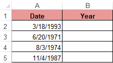
Example: There is a table with a list of dates and in each of them it is necessary to separate the value of only the year.

We introduce the original data in Excel.

To solve the problem, it is necessary to enter the formula in the cells of column B:

=YEAR(the address of the cell, from the date of which you need to isolate the year value)

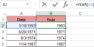
As a result, we extract years from each date.

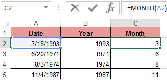
A similar example of the MONTH function in Excel:

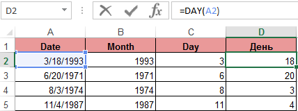
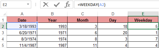
An example of working with functions DAY and WEEKDAY. The DAY function gets to calculate from the date the number of any day:

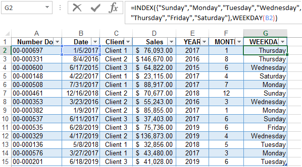
WEEKDAY function returns the number of the day of the week (1-Monday, 2-Tuesday …, etc.) for any date:

In the second optional argument of the WEEKDAY function, the number 2 may specified for our day of the week countdown format (Monday-1 through Sunday-7):

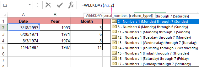
If you omit the second optional argument, then the default format will be used (English from Sunday-1 to Saturday-7).

Create a formula of the combination of the functions INDEX and WEEKDAY:

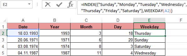
We obtain a more understandable form of the implementation of this function.



Examples of the practical use of functions for working with dates

These primitive functions are very useful when grouping data by: years, months, days of the week, and specific days.

Suppose we have a simple sales report:

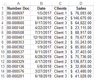
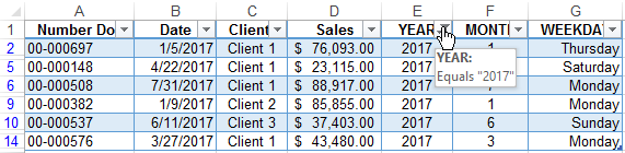
We need to quickly organize data for visual analysis without using pivot tables. To do this, we will bring the report into a table where it is convenient and quickly to group data by year, month and day of the week:

Now we have a tool to work with this sales report. We can filter and segment data by specific time criteria:

In addition, you can make a histogram to analyze the best-selling days of the week, to understand which day of the week has the largest number of sales:

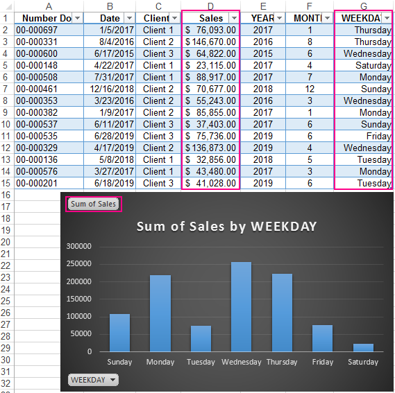
In this form, it is very convenient to segment sales reports for long, medium and short periods of time.

It should be immediately noted that in order to get the difference between the two dates, none of the above functions will help us. For this task, you should use a specially designed function DATEDIF:

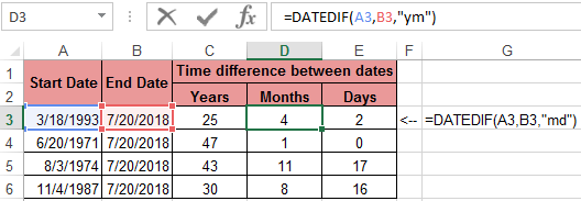
Download examples fo functions YEAR MONTH DAY WEEKDAY and DATEDIF

The type of values in the date cells requires a special approach to data processing. Therefore, you should use the appropriate type of function in Excel.

Whenever you enter a date in a cell, Excel automatically recognizes the format and converts the cell to a date cell.

So, Excel knows which part of the date you entered is the month, which is the year and which is the day.

This can be quite helpful in many ways. One particular benefit of this capability of Excel is that it lets you display the date in any format you want. It even lets you extract parts of the date that you need.

For example, you might find the day part of the date irrelevant and just need to display the month and year.

Since Excel already understands your date, you can easily extract just the month and year and display it in any format you like.

In this tutorial, we are going to see three ways in which you can convert date to month and year in Excel.

The Sample Data

Throughout this tutorial, we are going to be using the following set of dates. We will be converting these dates to month and year in Excel:

When working with dates, first and foremost, it is important to recognize the original format your Excel dates are in. For example, in the US format, dates usually begin with the month and end with the year (mm/dd/yyyy).

In the UK and other countries, dates begin with the day and end with the year (dd/mm/yyyyy). In still other places like China, Iran, and Korea, the order is completely flipped (yyyy/mm/dd).

Depending on your computer’s date settings Excel will treat parts of your date differently. So when entering the date, make sure you check the format and enter the date in the correct order. You don’t want the date 2/10 to be treated as October, the 2nd instead of February, the 10th!

Convert Date to Month and Year using the MONTH and YEAR function

The MONTH and YEAR functions can help you extract just the month or year respectively from a date cell. In order for this method to work, the original date (on which you want to operate) must be a valid Excel date. If not, then both these functions will return a #VALUE error.

Let’s see how you can extract the month from our sample data:

1. Click on a blank cell where you want the month to be displayed (B2)
2. Type: =MONTH, followed by an opening bracket (.
3. Click on the first cell containing the original date (A2).
4. Add a closing bracket )
5. Press the Return key.
6. This should display the month of the year corresponding to the original date. Copy this to the rest of the cells in the column by dragging down the fill handle or double-clicking on it.

You will see column B populated by the month of the year for all the dates of column A.

Now let’s see how you can extract the year from the same dataset:

1. Click on a blank cell where you want the year to be displayed (C2)
2. Type: =YEAR, followed by an opening bracket (.
3. Click on the first cell containing the original date (A2).
4. Add a closing bracket )
5. Press the Return key.
6. This should display the year corresponding to the original date. Copy this to the rest of the cells in the column by dragging down the fill handle or double-clicking on it.

You will see column C populated by the year corresponding to all the dates of column A.

Now let’s see how you can combine the results of the two to display both month and year in a nice format.

Let us say you want to display both month and year as “2-2018” for the date “02/10/2018”, and want to follow this pattern for all the dates.

1. Click on a blank cell where you want the new date format to be displayed (D2)
2. Type the formula: =B2 & “-“ & C2. Alternatively, you can type: =MONTH(A2) & “-” & YEAR(A2).
3. Press the Return key.
4. This should display the original date in our required format. Copy this to the rest of the cells in the column by dragging down the fill handle or double-clicking on it.

Now all your cells in column D2 have the new format:

Alternatively, if you want to display your month and year as 2/2018 instead, you only need to replace the “-“ in-between with a “/”. In this way, you can display the month and year in any format that you like.

Finally, if you want to just keep the converted values and want to remove the original dates and any intermediate columns that you created you need to first convert the formula results into constant values.

For this, copy the cells of column D and paste them as values in the same column (Right-click and select Paste Options->Values from the Popup menu). Now you can go ahead and delete columns A to C. You will be left with only the converted values that have the month and year.

Although this is quite an easy and intuitive way to convert dates to months and years, it is a less popular method. This is because this method does not provide a lot of flexibility compared to the other two methods we will show next.

Also read: How to Calculate the Number of Months Between Two Dates in Excel?

Convert Date to Month and Year using the TEXT Function

The TEXT function in Excel converts any numeric value (like date, time, and currency) into text with a specified format.

The syntax of the TEXT function is:

= TEXT (value, format_code)

Here,

• value is the numeric value or reference to the cell that you want to convert
• format_code is the format you want to convert the cell into

In the above example, the TEXT function applies the format_code that you specified on the value and returns a text string with that format. For example, if you have a date “2/10/2018” in cell A2, then =TEXT(A2, “mm/yyyy”) will return “02/2018”

There are a number of format codes that you can use. We have enlisted below the basic building blocks for the format codes:

Format Codes for Year:

You can use the following two basic format codes to represent year values:

• yy – two-digit representation of year (e.g. 20 or 12)
•  yyyy – four-digit representation of year (e.g. 2020 or 2012)

So, if you apply =TEXT(A2, yy) in our example dataset, it will return “18”.

If you apply =TEXT(A2, yyyy), then it will return “2018”.

Format Codes for Month of the Year:

You can use the following four basic format codes to represent month values:

• m – one or two-digit representation of the month (eg; 8 or 12)
• mm – two-digit representation of the month (eg; 08 or 12)
• mmm – month abbreviated in three letters (eg: Aug or Dec)
• mmmm – month expressed with the full name (eg: August or December)

So, if you apply =TEXT(A2, m) in our example dataset, it will return “2”.

• If you apply =TEXT(A2, mm), then it will return “02”.
• If you apply =TEXT(A2, mmm), then it will return “Feb”.
• If you apply =TEXT(A2, mmmm), then it will return “February”.

Let us see how we can apply the TEXT function to our sample dataset to convert all the dates to different formats.

We will first see how to convert the dates in column A to the format shown in column B in the image below:

Below are the steps to change the date format and only get month and year using the TEXT function:

1. Click on a blank cell where you want the new date format to be displayed (B2)
2. Type the formula:

   =TEXT(A2,”m/yy”)

3. Press the Return key.
4. This should display the original date in our required format. Copy this to the rest of the cells in the column by dragging down the fill handle or double-clicking on it.
5. Copy this column’s formula results by pressing CTRL+C or Cmd+C (if you’re on a Mac).
6. Right-click on the column and form the popup menu that appears, press Paste Values from the Paste Options.
7. This will store the formula results as permanent values in the same column. Now you can go ahead and remove column A if you want to.

The format code that you put in the formula (at step 2) will vary according to the format you want your month and year to appear in. Here are the format codes along with the type of result you will get when applied to cell A2:

Function	Result
=TEXT(A2, “mm/yy”)	02/18
=TEXT(A2, “mm-yy”)	02-18
=TEXT(A2, “mm-yyyy”)	02-2018
=TEXT(A2, “mmm, yyyy”)	Feb, 2018
=TEXT(A2, “mmmm, yyyy”)	February, 2018

So you see, you can use the TEXT function to convert your dates to any format of your choice. All you need to do is change the format code according to your requirement.

Note: Using this formula, your date gets converted to a text format. If you want to convert it back to a date format, you need to use the Format Cells feature.

Also read: How to Convert Text to Date in Excel?

Convert Date to Month and Year using Number Formatting

Excel’s Format Cell feature is a versatile one that lets you perform different types of formatting through a single dialog box.

Here’s how you can convert the dates in our sample dataset to different formats.

1. Select all the cells containing the dates that you want to convert (A2:A6).
2. Right-click on your selection and select Format Cells from the popup menu that appears. Alternatively, you can select the dialog box launcher in the Number group under the Home tab.
3. This will open the Format Cells dialog box. Click on the Number tab
4. Under Category on the left side of the box, select the Date option.
5. This will display a number of formatting options for date on the right side.
6. Select the format that you want. For example, if you want to display the first date in the format “Feb-18”, then select the matching format option.
7. If you don’t find an option for the format you want to use, then you can use the Custom option from the Category list on the left. This lets you convert the cell to a custom format.
8. Look if your format is available among the date format codes under Type. If not, you can type in your format code in the input box just below Type. So, if you want to display the first month in the format “2/18”, then type “m/yy”.
9. Click OK to close the Format Cells dialog box.

All your selected cells should now be formatted to your required format.

This method differs from the previous one (using the TEXT function) in four ways:

• With this method, you can perform the operation directly on the original cells.
• You can get your conversion done in one go. So you don’t need to have a separate cell to enter the formula, then paste by value and then delete the original cells (as you would need to if using the TEXT function).
• This method changes just the format of the original date, the underlying date, however, remains the same. So if you want to later recover the original date value (along with the day), you can easily access it. With the TEXT function method, however, the original date value is lost because the conversion changes the entire value of the date.
• The results you get from using this method are of type Date, rather than Text, so you can perform date operations on them directly without having to convert them.

These were three ways in which you can convert date to month and year in Excel. Using these you can convert your date to any format you need.

We hope you found our methods useful and that you will apply it to your own Excel data.

Other Excel tutorials you may like:

• How to Convert Decimal to Fraction in Excel
• How to Add Days to a Date in Excel
• How to Sort by Date in Excel (Single Column & Multiple Columns)
• How to Convert Serial Numbers to Date in Excel
• How to Convert Date to Day of Week in Excel
• How to Convert Month Number to Month Name in Excel
• How to Convert Days to Years in Excel (Simple Formulas)
• Convert Military Time to Standard Time in Excel (Formulas)
• Convert YYYYMMDD to MM/DD/YYYY in Excel

Sample Files

1. DATE Function

DATE function returns a valid date based on the day, month, and year you input. In simple words, you need to specify all the components of the date and it will create a date out of that.

Syntax

DATE(year,month,day)

Arguments

• year: A number to use as the year.
• month: A number to use as the month.
• day: A number to use as a day.

Example

In the below example, we have used cell references to specify the year, month, and day to create a date.

You can also insert arguments directly into the function to create a date as you can see in the below example.

And in the below example, we have used different types of arguments to see the result returned by the function.

2. DATEVALUE Function

DATEVALUE function returns a date after converting a text (which represents a date) into an actual date. In simple words, it converts a date into an actual date which is formatted as text.

Syntax

DATEVAUE(date_text)

Arguments

• date_text: The date which is stored as a text and you want to convert that text into an actual date.

Example

In the below example, we have inserted a date directly into the function by using double quotation marks. If you skip adding these quotation marks it will return a #NAME? error in the result.

In the below example, all the dates on the left side are in textual format.

1. A simple textual date that we have converted into a valid date.
2. A date with all three components (Year, Month, or Day) in numbers.
3. If there is no year in the textual date, it will take the current year as the year.
4. And if you have a month name is in alphabets and no year, it will take the current year as a year.
5. If you don’t have the day in your textual date it will take 1 as the day number.

3. DAY Function

DAY function returns the day number from a valid date. As you know, in Excel, a date is a combination of day, month, and year, DAY function gets the day from the date and ignores the rest of the part.

Syntax

DAY(serial_number)

Arguments

• serial_number: A valid serial number of the date from which you want to extract the day number.

Example

In the below example, we have used the DAY to simply get the day from a date.

And in the below example, we have used DAY with TODAY to create a dynamic formula that returns the current day number and it will update every time you open your worksheet or when you recalculate your worksheet.

5. DAYS Function

DAYS function returns the difference between two dates. It takes a start date and an end date and then returns the difference between them in days. This function was introduced in Excel 2013 so not available in prior versions.

Syntax

DAYS(end_date,start_date)

Arguments

• start_date: It is a valid date from where you want to start the days’ calculation.
• end_date: It is a valid date from where you want to end the days’ calculation.

Example

In the below example, we have referred the cell A1 as the start date and B1 as the end date and we have 9 days in the result.

Note: You can also use the subtract operator to get the difference between two dates.

In the below example, we have directly inserted two dates into the function to get the difference between them.

6. EDATE Function

EDATE function returns a date after adding a specified number of months to it. In simple words, you can add (with a positive number) or subtract (with a negative number) months from a date.

Syntax

EDATE(start_date,months)

Arguments

• start_date: The date from which you want to start the calculation.
• months: The number of months to calculate the future or the past date.

Example

Here we have used EDATE with different types of arguments.

• In the first example, we have used 5 as a several months and it has added exactly 5 months on 1-Jan-2016 and returned 01-June-2016.
• In the second example, we have used -1 month and it has given 31-Dec-2016, a date which is exactly 1 month back from 31-Jan-2016.
• In the third example, we have inserted a date directly into the function.

7. EOMONTH Function

EOMONTH function returns the end of the month date which is the number of months in the future or the past. You can use a positive number for a future date and a negative number for the past month’s date.

Syntax

EOMONTH(start_date,months)

Arguments

• start_date: A valid date from where you want to start your calculation.
• months: The number of months you want to calculate before and after the start date.

Example

In the below example, we have used EOMONTH with different types of arguments:

• We have mentioned 01-Jan-2016 as the start date and 5 months for getting a future date. As June is exactly 5 months after January, it has returned 30-Jun-2016 in the result.
• As I have already mentioned, EOMMONTH is smart enough to evaluate the total number of days in a month.
• If you mention a negative number, it simply returns a past date which is the number of months back you have mentioned.
• In the fourth example, we have used a date that is in text format and it has returned the date without returning any errors.

8. MONTH Function

MONTH function returns the month number (ranging from 0 to 12) from a valid date. As you know, in Excel, a date is a combination of day, month, and year, MONTH gets the month from the date and ignores the rest of the part.

Syntax

MONTH(serial_number)

Arguments

• serial_number: A valid date from which you want to get the month number.

Example

In the below example, we have used a MONTH in three different ways:

• In the FIRST example, we have simply used date and it has returned the 5 in the result which is the month number of MAY.
• In the SECOND example, we have supplied the date directly in the function.
• In the THIRD example, we have used the TODAY function to get the current date and MONTH has returned the month number from it.

9. NETWORKDAYS Function

NETWORKDAYS function returns the count of days between the start date and end date. In simple words, with NETWORKDAYS you can calculate the difference between two dates, after excluding Saturdays and Sundays, and holidays (which you specify).

Syntax

NETWORKDAYS(start_date,end_date,holidays)

Arguments

• start_date: A valid date from where you want to start your calculation.
• end_date: A valid date up to which you want to calculate working days.
• [holidays]: A valid date that represents a holiday between the start date and end date. You can refer to a cell, range of cells, or an array containing dates.

Example

In the below example, we have specified 10-Jan-2015 as a start date and 20-Feb-2015 as an end date.

We have 41 days between these two dates, out of which 11 days are weekends. After deducting those 11 days it has returned 30 working days.

Now in the below example with the same start and end dates, we have specified a holiday and, after deducting 11 days of the weekend and 1 holiday it has returned 29 working days.

Again with the same start and end dates, we have used a range of three cells for holidays to deduct from the calculation and, after deducting 11 weekend days and 3 holidays which I have mentioned It has returned 27 working days.

10. NETWORKDAYS.INTL Function

NETWORKDAYS.INTL Function returns the count of days between the start date and end date. Unlike NETWORKDAYS, NETWORKDAYS.INTL lets you specify which days you want to exclude from the calculation.

Syntax

NETWORKDAYS.INTL(start_date,end_date,weekend,holidays)

Arguments

• start_date: A valid date from where you want to start your calculation.
• end_date: A valid date up to which you want to calculate working days.
• [weekend]: A number represents to exclude weekends from the calculation.
• [holidays]: A list of dates that represents the holidays you want to exclude from the calculation.

Example

In the below example, we have used 01-Jan-2015 as a start date and 20-Jan-2015 as an end date. And we have specified 1 to take Sunday – Saturday as the weekend. The function has returned 14 days after excluding 6 weekend days.

Below, we have used the same dates. And I have used 11 in for weekend days which means it will only consider Sunday as a weekend. Along with that, we have also used 10-Jan-2015 as a holiday.

We have 3 Sundays between both dates and a holiday. After excluding all these days the function has returned 16 days in the result. Here in the below example, we have used range to specify holidays. If you have more than one date for the holidays you can refer to an entire range.

Quick Tip: If you want to create a dynamic range for holidays, you can use a table for that. If you want to choose custom days to count as working days or weekends, you can use the below format in the weekend argument.

Here, 0 represents a working day and 1 represents a non-working day. And, seven numbers represent 7 days of the week.

11. TODAY Function

The TODAY function returns the current date and time as per the system’s date and time. The date and time returned by the NOW function update continuously whenever you update anything in the worksheet.

Syntax

TODAY()

Arguments

• In the TODAY function, there is no argument, all you need to do is enter it in the cell and hit enter, but be careful as TODAY is a volatile function which updates its value every time you update your worksheet calculations.

Example

In the below example, we have used TODAY  with other functions to get the current month number, current year, and current day.

12. WEEKDAY Function

WEEKDAY function returns a day number (ranging from 0 to 7) of the week from a date. In simple words, the WEEKDAY function takes a date and returns the day number of that date’s day.

Syntax

WEEKDAY (serial_number, [return_type])

Arguments

• serial_number: A valid date from which you want to get the week number.
• [return_type]: A number that represents the day of the week to start the week.

Example

In the below example, we have used a WEEKDAY with TODAY to get a dynamic weekday. It will give you the weekday whenever the current date changes. You can use this method in your dashboards to trigger some values which need to change when weekday change.

In the below example, we have used WEEKDAY with IF to create a formula that first checks the weekday of date and return “Weekday” or “Weekend” basis on the value return from WEEKDAY.

13. WEEKNUM Function

WEEKNUM function returns the week number of a date. In simple words, WEEKNUM returns the week number of dates that you specify ranging from 1 to 54.

Syntax

WEEKNUM(serial_number,return_type)

Arguments

• serial_number: A date for which you want to get the week number.
• [return_type]: A number to specify the starting day of the first week of the year. You have two systems to specify the starting date of the week.

Example

In the below example, we have used TODAY with WEEKNUM to get the week number of the current date. It will update the week number automatically every time the date changes.

In the below example, we have added the text “Week-” with the week number for a meaningful result.

14. YEAR Function

YEAR Function returns the year number from a valid date. As you know, in Excel a date is a combination of day, month, and year, and the YEAR function gets the year from the date and ignores the rest of the part.

Syntax

YEAR(date)

Arguments

• date: A date from which you want to get the year.

Example

In the below example, we have used the year function to get the year number from the dates. You can use this function where you have dates in your data and you only need the year number.

And in the below example, we have used today function to get the year number from the current date. It will always update the year whenever you recalculate your worksheet.

Bottom line: With Valentine’s Day rapidly approaching I thought it would be good to explain how you can get a date with your Excel skills.  Just kidding! 🙂  This post and video explain how the date calendar system works in Excel.

Skill level: Beginner

Dates in Excel can be just as complicated as your date for Valentine’s Day.  We are going to stick with dates in Excel for this article because I’m not qualified to give any other type of dating advice. 🙂

Video Tutorial on How Dates Work in Excel

The following is a video from The Ultimate Lookup Formulas Course on how the date system works in Excel.

Watch the Video on YouTube

There are over 100 short videos just like the one above included in the Ultimate Lookup Formulas Course.

This course has been designed to help you master Excel’s most important functions and formulas in an easy step-by-step manner.

The Ultimate Lookup Formulas course is now part of our comprehensive Elevate Excel Training Program.

Click Here to Learn More About Elevate Excel

What is a Date in Excel?

I should first make it clear that I am referring to a date that is stored in a cell.

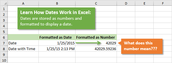
The dates in Excel are actually stored as numbers, and then formatted to display the date.  The default date format for US dates is “m/d/yyyy” (1/27/2016).

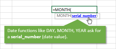
The dates are referred to as serial numbers in Excel.  You will see this in some of the date functions like DAY(), MONTH(), YEAR(), etc.

So then, what is a serial number?  Well let’s start from the beginning.

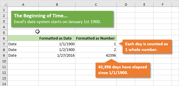
The date calendar in Excel starts on January 1st, 1900.  As far as Excel is concerned this day starts the beginning of time.

Each Day is a Whole Number

Each day is represented by one whole number in Excel.  Type a 1 in any cell and then format it as a date.  You will get 1/1/1900.  The first day of the calendar system.

Type a 2 in a cell and format it as a date.  You will get 1/2/1900, or January 2nd.  This means that one whole day is represented by one whole number is Excel.

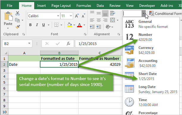
You can also take a cell that contains a date and format it as a number.

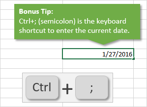
For example, this post was published on 1/27/2016.  Put that number in a cell (the keyboard shortcut to enter today’s date is Ctrl+;), and then format it as a number or General.

You will see the number 42,396.  This is the number of days that have elapsed since 1/1/1900.

Date Based Calculations

It is important to know that dates are stored as the number of days that have elapsed since the beginning of Excel’s calendar system (1/1/1900).

When you calculate the difference between two dates by subtraction, the result will be the number of days between the two dates.

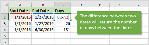
1/27/2016 – 1/1/2016 = 26 days

6/30/2016 – 1/1/2016 = 181 days

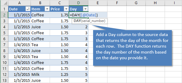
There are a lot of Date functions in Excel that can help with these calculations.  Last week we learned about the DAY function for month-to-date calculations with pivot tables.

We won’t go into all the date functions here, but understanding that the serial number represents one day will give you a good foundation for working with dates.

What About Dates with Times?

Do you ever work with dates that contain time values?

These dates are still stored as serial numbers in Excel.  When you convert the date with a time to the number format, you will see a decimal number.

This decimal is a fraction of the day.

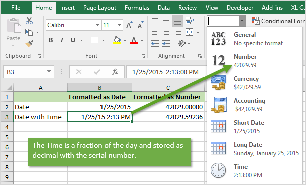
One hour in Excel is represented by the number: 1/24 = 0.04167

One minute in Excel is represented by the number: 1/(24*60) = 1/1440 = 0.000694

So 8:30 AM can be calculated as: (8 * (1/24)) + (30 * (1/1440)) = .354167

An easier way to calculate this is by typing 8:30 AM in a cell, then changing the format to Number.

So if you are running a half hour late and want to let your boss know, text him/her and say you will be there at 0.354167. 🙂

Checkout my article on 3 ways to group times in Excel for more date time based calculations.

Don’t Talk About Excel Dates with Your Date

Unless your Valentine shares a similar passion for Excel, I strongly recommend NOT sharing this information on your date.

I remember the first time I met my wife, and told her I worked in finance.  The first word out of her mouth was, “BORING!”.  Awe… it was love at first sight… LOL 🙂

But you should now be able to use Excel to determine how many days it has been since you last spoke to your date.  That’s the only dating advice I can give.

Please leave a comment below with any questions on Excel dates.  Thanks!

All Excel’s Date Functions Explained + Time Functions Too! [+5500 words]

All Excel’s Date and
Time Functions Explained!

Written by co-founder Kasper Langmann, Microsoft Office Specialist.

This is the complete guide to date and time in Excel.

It’s a whopping +5500 words (!), so be sure to bookmark it.

The first part of the guide shows you exactly how to deal with dates in Excel.

I will show you how to perform calculations involving dates. We’re also going to look at some of Excel’s (awesome) built-in functions. These allow you to extract just what you need from data that includes dates.

In the second part of the guide, I’ll show you how to work with time data in a spreadsheet.

This is going to be a lot of fun. Grab a cup of coffee, and let’s start rolling!

Kasper Langmann, Co-founder of Spreadsheeto

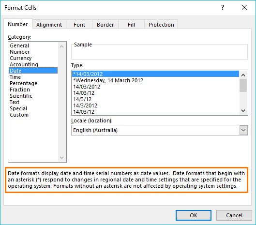
• 7: Date formatting

  • What is date formatting?
  • How to use other date formats (from the ‘Format Cells’ dialog box)
  • How to use custom date format
  • Turn text into dates with the DATEVALUE function
  • How to auto populate date in Excel when a cell is updated
  • How to insert a date picker in Excel

Get your FREE exercise file

Before you start:

Throughout this guide, you need a data set to practice.

I’ve included one for you (for free).

Download it right below!

Introduction to
calculations with dates

When analyzing and manipulating date information in Excel, you have several formatting options.

In other words, you can display your data in many ways.

Most of the time, Excel will know that you are entering a date when you key in the data like the following:

• 1/1/2017
• January 1, 2017
• 1-Jan

The clearest sign that Excel has stored your data in a cell as a date is that it should be right-aligned in the cell.

Kasper Langmann, Co-founder of Spreadsheeto

Below are a few examples of the various formats that Excel displays dates in.

But the key is that they are all aligned to the right of the cell.

Contrast column A with column B (where the cells are formatted as text). They show the same information.

But, the alignment to the left side of the cell indicates that they are not formatted as a date. As you will soon see, this presents problems when performing calculations with dates.

Kasper Langmann, Co-founder of Spreadsheeto

One important note about how Excel stores dates:

To use dates in calculations, Microsoft Excel stores dates as serial numbers.

These are the sequential number of the day in relation to the starting date of January 1, 1900.

So, think of January 1, 1900, as serial number 1.

January 1, 2016, would be serial number 42370 as it’s 42,370 days after January 1, 1900.

For this reason, dates need to be in a date format rather than text format. If stored in text format, their serial number will not be stored in Excel. This is a no-go as you need these serial numbers when you want to perform calculations involving dates.

Kasper Langmann, Co-founder of Spreadsheeto

How to add time to dates in Excel

Now you know the fundamentals of date formatting versus date data formatted as text. Let’s look at some calculations you can do with dates.

First, why don’t we look at how to add days to a date?

Kasper Langmann, Co-founder of Spreadsheeto

How to add days to a date

Adding days to a date is very simple, straightforward, and intuitive.

All you need to do is add the number of days as a single number to the date or cell reference containing the date.

The following figure illustrates just how simple it is to add 1 day or 90 days to a date.

How to add months to a date

If you need to add a month or several months to your date, the process is a bit more complicated.

For this calculation, you will need to call upon the built-in Excel function, EDATE. The syntax for EDATE is so simple, that you will pick it up in no time at all.

Kasper Langmann, Co-founder of Spreadsheeto

Here’s its syntax:

=EDATE(start_date, months)

The function requires 2 arguments: ‘start_date’ and ‘months’.

The first, ‘start_date’, is simply the date we are adding months to.

The second, ‘months’, is the number of months we would like to add to the date.

Look at the figure below to see just how easy it is to calculate a new date by adding 6 months and 9 months to the start date.

How to add years to a date

So, what about calculating the addition of years to your original date?

For this, you need to use a few more functions. But, as noted before, this is super intuitive so don’t let the length of these formulas fool you.

Kasper Langmann, Co-founder of Spreadsheeto

The first function we need to focus on is DATE.

The syntax for DATE is also incredibly simple and intuitive:

=DATE(year, month, day)

But, for our purposes, we can use the YEAR, MONTH, and DAY functions along with DATE.

These functions extract the correct data from our original date. This ensures appropriate use of our final DATE formula.

For example, applying MONTH to a cell reference of our original date will extract the month data. The same is true for YEAR and DAY.

So, we will place these functions in the appropriate argument within the DATE function. And if we want to add 1 year to the date, we simply place a ‘+1’ after the YEAR function in the ‘year’ argument of the DATE function.

Kasper Langmann, Co-founder of Spreadsheeto

That was a lot, so let’s look at the following figure to see it in action.

Notice row 18 and column C of the worksheet.

The ‘year’ argument of the ‘DATE’ function is substituted by the function ‘YEAR(A18)+1’.

This tells the DATE function that we want the year only from the date data in A18 (or 2017) – and that we want to add ‘1’ to it (or 2018).

How to subtract dates

Adding time to a date is super useful.

But what if you had a report where you needed to calculate the difference between dates?

This is where we turn our attention to subtracting dates…

Kasper Langmann, Co-founder of Spreadsheeto

Find the difference between two dates

To find the difference between two dates, we want to turn our attention to the DATEDIF function.

The most important thing you need to know about DATEDIF is that it is a hidden function. What that means is that it will not be found in the visible list of Excel functions on the formula tab.

Kasper Langmann, Co-founder of Spreadsheeto

This requires you to type the formula in its entirety.

There will be no tooltip hint as you begin to type the function.

Let’s look at the syntax:

=DATEDIF(start_date, end_date, unit)

There are three arguments for the DATEDIF function:

• start_date: This is the initial date of the period among the two you are calculating the difference between.
• end_date: This is the latest date of the two.
• unit: This is the unit in which you want the function to return the difference by. More on units right below…

The ‘unit’ argument gives you a choice of several formats to return your results from DATEDIF.

• y – The number of complete years between dates.
• m – The number of complete months between dates.
• d – The number of days between dates.
• md – The number of days ignoring months and years.
• yd – The number of days ignoring years.
• ym – The number of months ignoring days and years.

So, let’s look at a few examples using DATEDIF in various forms.

Kasper Langmann, Co-founder of Spreadsheeto

In our example, you can use literal dates if they are enclosed in double quotes.

You can also use the serial number format as shown in rows 4 and 5.

Now note the difference in the returned value between row 2 and 3. The ‘start_date’ and the ‘end_date’ are unchanged. But, our results are different. The first formula returns the total number of days between the dates.

Kasper Langmann, Co-founder of Spreadsheeto

But in the second example, we use ‘md’ for the unit argument. ‘md’ is the difference between the dates in days – ignoring the months and years. That is 15 minus 1, or 14 days.

You can also calculate the difference between two dates in cells.

To do this, place the cell reference of your dates in the ‘start_date’ and ‘end_date’ arguments.

One (last) important thing to note about using DATEDIF:

The ‘end_date’ argument must always be later than the ‘start_date’ or you will get the ‘#NUM!’ error.

Use today’s date in Excel

Now let’s turn our attention to some tricks and shortcuts involving the current date.

Often, you need to work with the current (today’s) date.

There are some nifty tricks that allow you to do this without typing in the entire date manually.

Let’s look at them!

Use date that updates itself with the TODAY function

One of the simplest ways to input today’s date into a cell is to use the TODAY function.

Do this by typing ‘=TODAY()’ into a cell.

This places the current date into the cell dynamically. So, that cell would have tomorrow’s date in it if you reopen the file tomorrow.

You can also nest the TODAY function within the DAY or MONTH function. This return only the current day or current month in a cell. Refer to the following figure to see the TODAY function in action.

Kasper Langmann, Co-founder of Spreadsheeto

Insert static current date in Excel using shortcuts

You can also insert the current date using keyboard shortcuts.

For the current date, press the following key combination:

Ctrl + ;

To insert both the date and the time, press the previous keyboard shortcut. Then press the following combination:

Ctrl + Shift + ;

These shortcuts enter static dates and times. This opposed to the dynamic date that the TODAY function returns.

Subtract a date from the current date

You can use the current date in a calculation like subtracting.

You replace the ‘start_date’ argument in the DATEDIF formula.

Above image shows how to substitute the TODAY function for a literal date value or cell reference for the ‘start_date’ OR the ‘end_date’.

Remember the rule that the ‘end_date’ must be later than the ‘start_date’ still applies.

Using the TODAY function in a calculation is useful when you need to track a time period dynamically. Say you need to calculate some sort of countdown to a deadline. Using the TODAY function in your calculation is the perfect way to do this.

Kasper Langmann, Co-founder of Spreadsheeto

You can also use the keyboard shortcut to insert the current date if you need to insert the static date. This is a quicker and more efficient way to insert today’s date.

Retrieving numbers from dates
with Date functions

There are often situations where you need to retrieve numbers from dates.

But, you might not have the need for an entire date.

Let’s say you have a report. Here you want to separate the different elements of the date for filtering by a single element of the date – like the month or year.

Here’s how to go about doing that 🙂

Use the DAY function to find the day of a date

To isolate only the day of the full date, we use the DAY function.

There is a single argument for the DAY function:

=DAY(serial_number)

You probably know by now that ‘serial_number’ is the date.

This argument can be the actual serial number form of the date or the literal date in double quotes. It can also be a cell reference like in the following example.

Look at above picture again. Notice that regardless of the format of your original date, the DAY function returns the value ‘14’.

Use the MONTH function to find the month of a date

If you need to isolate the number value for the month of your original date, you can use the MONTH function.

It works the same way the DAY function works:

=MONTH(serial_num)

Use the YEAR function to find the year of a date

Now we move onto the function that retrieves the number value for the year part of the date.

The syntax for the ‘YEAR’ function is like the DAY and MONTH functions syntactically.

=YEAR(serial_num)

You already know how to retrieve the day and month number values. It’s the exact same concept when using the ‘YEAR’ function.

Use the WEEKDAY function to find the day of the week

You can also retrieve the number value for the day of the week from a date.

The WEEKDAY function returns the number that corresponds to the day of the week. For instance, 1 for Sunday, 2 for Monday, 3 for Tuesday, and so on.

Kasper Langmann, Co-founder of Spreadsheeto

Here’s its syntax:

=WEEKDAY(serial_num, [return_type])

The syntax for WEEKDAY requires the ‘serial_number’ argument.

It also allows for an optional argument: ‘return_type’.

This allows you to choose a different start and end date for your week.

That means that the returned value will align with that chosen sequence.

Below you can see the list of different ‘return_type’ values that Excel allows.

In the following examples, note the value differences returned by the formula based on the ‘return_type’ argument.

The different selections for the ‘return_type’ in the formulas return very different weekday values.

These depend on the first day of the week that corresponds to those ‘return_type’ values.

Use the WEEKNUM function
to find out the week number

Another interesting built-in function is the WEEKNUM function.

WEEKNUM retrieves the number value for the week of the year that the original date falls within (1 – 52).

So, if the original date is between January 1 and January 7, the WEEKNUM value would be ‘1’.

If the date is between December 25 and December 31, WEEKNUM would return the value ‘52’.

=WEEKNUM(serial_number, [return_type])

The ‘return_type’ argument corresponds to different days you can choose as the start day. This changes the week number based on what day of the week that the ‘return_type’ sets as the first day of the year.

Kasper Langmann, Co-founder of Spreadsheeto

Our date falls on a Monday.

The result of the WEEKNUM formula will be different if the ‘return_type’ argument is ‘1’ (Sunday) versus ‘12’ (Tuesday).

This can be useful since the calendar year begins on different days of the week. This comes in handy if want to calculate the week number based on the first full week of the year.

Kasper Langmann, Co-founder of Spreadsheeto

This can be a very useful function.

Consider a situation in which you needed a weekly countdown. Simply calculate the difference between dates using the WEEKNUM function.

Use the WORKDAY function to calculate the number of working days between two dates

Another useful function is the WORKDAY function.

This function returns a day that is some number of workdays into the future or before some date. A “workday” is days excluding weekends and any holidays that are specified.

The function requires two arguments and has an optional third.

=WORKDAY(start_date, days, [holidays])

• start_date – this required argument is the date from when you want to count the number of workdays
• days – this required argument is the number of days from the start date you want a count of. Using a negative number will give you the date that many workdays before your start date.
• holidays – this argument is optional. This allows you to add holiday dates in the formula for the WORKDAY function to skip along with weekends.

This is a bit more complex than the functions we have been discussing. Let’s look at a few examples to help the concept of the WORKDAY function sink in.

Kasper Langmann, Co-founder of Spreadsheeto

First, note that we have listed 3 holiday dates in cells A8, A9, and A10. We will be using these in our examples for the ‘holiday’ argument to exclude along with weekends.

On row 2, we want to know the date that is 90 workdays from Monday, November 14, 2016.

Excluding the weekends and holidays (A8:A10), this will be Tuesday, March 21, 2017 according to the WORKDAY function.

On row 3, we can instantly see the effect of weekends and holidays on the outcome of our formula. We want the date that is 2 workdays from Wednesday, November 23, 2017.

Because of the holiday on Thursday, November 24 – and the weekend days Saturday and Sunday – the result is Monday, November 28, 2016.

This example illustrates how powerful the WORKDAY function can be. It calculates something very simple. Yet, if done manually, this is a very cumbersome process.

Kasper Langmann, Co-founder of Spreadsheeto

The third example in the figure illustrates how to use WORKDAY to find a date before the start date.

We want to know the date that is 20 workdays before Monday, January 17, 2017.

So, our DAY argument needs to be a negative value (-20).

Again, note the result considers weekend days as well as a couple of holidays.

How to auto fill dates

In this section, we are going to cover how to work with sequences of dates. This time by using the autofill capability of Microsoft Excel.

You can use Autofill in 2 ways.

The first is to double-click the fill handle. The fill handle is a small square that appears in the lower right corner of a highlighted cell.

The second option is to simply drag the handle to the desired cell. Note the fill handle for the highlighted cell in the following figure.

The fill handle also offers some more options.

Try to right-click and drag outside the selection a bit.

We will focus on the selections that fill elements of the date like days, weekdays, months, and years.

Insert dates that increase by one day

To insert dates that increase by one day in a column, you can simply grab the fill handle.

Then drag it down as many rows as you need dates for.

One thing to take note of is that as you do this, Excel shows the incremented date as you drag the range.

So, you can see just what date you are at as you expand the range.

Once you release the fill handle, your range is now filled with dates.

These dates increment in one-day intervals.

Insert dates that increase by weekdays

But what if you wanted to increment a wide range of dates by weekdays only?

This is easily done by selecting ‘Fill Weekdays’ from the ‘Autofill Options’ that appears once you fill the dates down.

Once you select ‘Fill Weekdays’, Excel automatically excludes any weekend dates from the range.

Insert dates that increase by months and years

You can also use the ‘Autofill Options’ to increase months and years.

Select the fill option you need once you fill the dates down to the last cell of your range.

Insert dates that increase by several days

I’m sure you can think of other custom intervals (dates) you might like to fill down your column (or row, for that matter).

Microsoft Excel allows for a little of that also.

So, what if you wanted to increment every other day? Or what about every 3 months?

These other intervals are available using auto fill. Drag down the dates by using the fill handle. Then right click and hold on the fill handle while moving the cursor slightly outside the range. Now release until you see the options menu.

Kasper Langmann, Co-founder of Spreadsheeto

Click on ‘Series…’. The Series dialog box will now open.

This gives you several options for customizing the intervals of your dates.

For our example of every other day, you can select a Step value of ‘2’.

Leave everything else as it is.

Date formatting:
Make a date easy to interpret

In the beginning of this tutorial, I told you about the differences between text format and date format.

Now, we’re going to take a deeper dive into formatting of dates. We can represent date data in different date formats. These are easily adjusted according to our preferences and needs.

Kasper Langmann, Co-founder of Spreadsheeto

Also, remember our point earlier, that Excel stores date data as serial number.

So, no matter what date format you choose, Excel still recognizes it as a serial number.

What is date formatting?

Date formatting offers you choices on how you want to represent the date data in your worksheets.

Let’s look at our original example at the beginning of this tutorial.

We can see in the Number group of the Home tab that our data cells are all formatted as Date.

If you take the same data and place it into another column, something interesting happens.

In the cells that are formatted as ‘General’, you’d see the dates serial numbers.

If you run into this in your own spreadsheets, you must know how to fix this…

It’s quite simple, you just need to know how to reformat those cells into the Date format that you need.

For this example, let’s reformat to ‘Short date’.

Highlight the cell containing the serial number. Click on the drop-down arrow to see all the available formats in the Number group of the Home tab.

Select ‘Short Date’ from the dropdown and now the serial number will be converted from ‘General’ format to a date format that you recognize.

How to use other date formats
from the ‘Format Cells’ dialog box

You’ve now seen how to change date data formatted as ‘General’ to the ‘Short Date’ format.

Now we look at some other date formats that Excel also offers…

You already know how to change to a date format from the ribbon but you can also use the ‘Format Cells’ dialog box.

The first step is to find the cell that contains the serial number you want to reformat.

Then, right-click on the cell.

Select ‘Format Cells’ from the menu that appears.

From the Format Cells dialog box, select ‘Date’ in the Category box.

This reveals the different standard date format types available in Excel.

You find these formats in the Type box on the right side of the Format Cells dialog box. As you change Type selections, you can view a sample of the actual value in the cell you have selected in the Sample box.

Kasper Langmann, Co-founder of Spreadsheeto

Decide on the ‘Type’ you want.

Then click ‘OK’ and the serial number now changes to the date format type you selected.

How to use custom date format

Even with all the date types Excel offers, you can still format your date data with your own custom format.

It is pretty simple to do…

Follow the same steps as we did with the previous example.

But, instead of choosing ‘Date’ in the Category box in the Format Cells dialog box, select ‘Custom’.

Take a second look at the picture above.

Here the Format Cells dialog box shows the current format of the cell in the Type and Sample boxes.

Now you can select from the various default types available. You can also edit those types in the Type box or type in one that is completely custom.

Kasper Langmann, Co-founder of Spreadsheeto

Let’s clear out the Type box…

And then type “mm-dd-yyyy”  into that box:

Again, note that as we do this, the Sample box shows us our exact data as it will look under our new custom format. Click ‘OK’ and you are done creating your own custom date format.

Kasper Langmann, Co-founder of Spreadsheeto

Turn text into dates with the DATEVALUE function

Another method for converting dates in text format is to use a function called DATEVALUE.

This function converts text string dates to their appropriate serial numbers.

These serial numbers are, as you know by now, the way Excel recognizes dates. You can format this output according to the methods I’ve shown you in the prior sections.

Kasper Langmann, Co-founder of Spreadsheeto

The DATEVALUE syntax is simple:

=DATEVALUE(date_text)

So, let’s look at a few examples of cells containing dates that are in text string form.

Let’s use the DATEVALUE function in the column next to these cells.

Here it’s easy to see if the cells return the serial numbers we expect.

If your text date is before the year 1900, the DATEVALUE function will return the ‘#VALUE!’ error.

That’s because Excel recognizes dates as serial numbers beginning at January 1, 1900.

If your text date doesn’t contain a year, the DATEVALUE function defaults to the current year from your system clock.

How to auto populate date when a cell is updated

What if you wanted to make sure each time a cell’s data got updated, you knew when it was updated?

You could input the date and time manually in the cell next to it.

But what if you wanted to automate that process?

That way you’ll never forget to do it. Also, you would mitigate the chances for a data entry error.

There are several ways to approach this. One of the best ways is to use VBA to create a worksheet change event. It is a macro that automatically runs when a cell’s value changes.

Kasper Langmann, Co-founder of Spreadsheeto

A quick recommendation:

Excelribbon.tips.net has written an awesome guide that demonstrates a worksheet change event. Make sure to check it out!

How to insert a date picker in Excel

Another cool thing you can do in Excel with dates is to create a date picker. This allows users to choose a date from a preset dropdown calendar. That way they don’t have to input the date by hand.

This is actually a pretty complex proposition in Excel. But if you want to see a date picker and a bit about how one can be created using VBA. Contextures has an amazing guide to do it right here.

Calculations with Time

Maybe you need to quantify elapsed time for tasks or projects?

Or perhaps you need to insert a time rather than a date in your data?

There are many parallels between the techniques of working with dates and time.

How to add time in Excel

Let’s look at a scenario where you have documented the total time it took for two different tasks in Excel.

Now you want to add those together to get your total time worked.

This is as simple as clicking on the cell below the task times and pressing Alt + = to autosum the times.

Now let’s look at a scenario where you have the times worked for a full workweek that you need to add together for a total.

If we autosum once again, we immediately notice a problem.

We know by simple inspection that these workday time values add up to more than 12 hours and 52 minutes.

Excel can display times in a variety of ways. For instance, hours and minutes, 12-hour format, and 24-hour format, and several others.

Kasper Langmann, Co-founder of Spreadsheeto

What we need to do in our current situation is to right click on the cell where our auto sum formula is.

Then select Format Cells like we did with dates.

Then select ‘Custom’ from the Category box and clear the Type box.

Then in the Type box, type ”[h]:mm”.

Click ‘OK’ and you should have the correct total of hours for the week now.

How to find the difference between two times

Finding the difference between times is not quite as simple as adding times together.

Let’s look at a situation where we have a start time and an end time and we want to calculate the total elapsed time.

In cell B4, type the formula ‘=(B3-B2)*24’.

This subtracts the end time from the start time and then multiplies both by 24.

The multiplication by 24 is required since Excel recognizes times as a fraction of a full 24-hour day.

Our result is a numerical value and we choose to set it to two decimal places to show fractions of a full hour.

If you want to see the elapsed time in the actual hours and minutes, here’s what to do.

Remove the ‘*24’ and format using the custom format we created in the previous example adding times ([h]:mm).

Find current time in Excel

The NOW function allows you to insert the current time based on your computer’s system clock.

NOW returns the current date and time whereas TODAY returns the current date only.

But we can use NOW and format our cell so that it only shows the time but not the date.

Insert static current time with shortcuts

You’ve already seen the keyboard shortcut for entering in the static current date as well as entering the static current time.

Since we are discussing time data, I’ll show you how to use a keyboard shortcut to enter the static current time.

All you must do is press the following keyboard combination:

Ctrl + Shift + ;

Again, this contrasts with using the NOW function because it is static rather than dynamic.

This keyboard shortcut inserts the exact time you pressed the keyboard shortcut. It will remain that time unless you manually change it.

Retrieve seconds, minutes and hours

Let’s look at retrieving parts of time data.

This is very much the same as when you retrieved the month, day, and year, from dates. We are going to retrieve the seconds, minutes, and hours with some built-in functions available in Excel.

If you want to retrieve the seconds from a time value in Excel, you use the built-in SECOND function.

There is a single required argument for this function: ‘serial_number’.

=SECOND(serial_number)

Let’s look at a few simple examples to see this function in action:

For times that don’t display the seconds, the SECOND function still retrieves the seconds from the serial number of the date.

If you need to retrieve the minutes from your time data, you want to use the MINUTE function. Like with SECOND function (and others), there is only the required ‘serial_number’ argument.

=MINUTE(serial_num)

Now we will take the same time data we used for the SECOND function and use the MINUTE function.

The last thing we will look at is the HOUR function. Nothing new on the syntax.

=HOUR(serial_number)

One thing to note about the HOUR function is that it returns a value for the hour based on 24 hours.

So, if you want your HOUR function to return the hour in an AM/PM fashion, subtract 12 from your function if it is a time later than 12 PM.

Formatting time: What is it?

Just like with dates, there are several different format types for time data.

In fact, our examples so far have demonstrated a few of these different formats.

You may want to display times in 12-hour format or 24 hours. You might want your 12-hour format times to show AM and PM, or you may not.

Kasper Langmann, Co-founder of Spreadsheeto

You find the default time format types by right-clicking a cell.

Then select Format Cells.

Note in the figure above how many variations you can choose from. You can always create your own custom format by selecting ‘Custom’ from the Category list.

How to use and change time formatting

Now we have reviewed how you select different time formats.

Let’s look at a few examples of the different types.

We will look at 3 different selections from those available in the types for time formats.

The first thing we need to do to change format is to right click on the range of dates we want to reformat. Then select Format Cells.

Once the Format Cells dialog opens, select ‘Time’ from the Category box. Then in the Type box select ‘*1:30:55 PM’.

The asterisk in ‘*1:30:55 PM’ indicates that this format changes to the Region settings on your computer.

Any changes to the Windows time format settings will reflect in Excel. But only for the times formatted with a format preceded by an asterisk.

So, we format column B times as ‘*1:30:55 PM’ and then two other formats in columns C and D for the sake of contrast. Look at the different format variations in the following figure.

Kasper Langmann, Co-founder of Spreadsheeto

Turn text into time with the TIMEVALUE function

The DATEVALUE function converts dates in text string form to date formatting.

Like DATEVALUE, the TIMEVALUE function converts text string time data to actual time format.

See the syntax here:

=TIMEVALUE(text_time)

The ‘text_time’ argument is required. It is simply the text string date that you need to convert to time format.

One thing to recall is that Excel recognizes time as a fraction of 24 hours. For instance, 12 pm would be interpreted by Excel as .5 since it is the halfway point of the 24-hour day.

Kasper Langmann, Co-founder of Spreadsheeto

So, when you use the TIMEVALUE function, you won’t get a time.

Rather, it returns a decimal number value that is a fraction of the entire day.

If you multiply the TIMEVALUE result by 24, you get a more accurate interpretation of the time (albeit still in decimal format).

But if you reformat the TIMEVALUE result to a time format, you are good to go.

You will have changed a text string time to a true time format that Excel will now recognize as time instead of text.

Wrapping up

There it is, the most comprehensive guide to date and time in Excel.

It’s taken us tons of hours and resources to publish. Feel free to share it along with anyone who needs to brush up their dates and times 😊

If you enjoyed this tutorial, I’m sure you’ll love this…

Kasper Langmann2020-05-11T13:30:38+00:00

The objective of this post is to teach you how Excel handles date and time and provide you with all the tools you will need.

It’s designed to be read in conjunction with the accompanying Excel file, which you can download below.

Download the Files

Regional Settings

When reading this post keep in mind that my regional settings format dates as dd/mm/yyyy and so the screenshots throughout this post are in this format. However, if you open the accompanying Excel file you may see some dates have switched to match your regional settings, which may be different to mine e.g. mm/dd/yyyy.

Dates and times with a format that begins with an asterisk (*) automatically update based on your PC’s regional settings. You can see an example in the Format Cells dialog box below:

Ok, let’s crack on.

Excel Date and Time 101

Excel stores dates and time as a number known as the date serial number, or date-time serial number.

When you look at a date in Excel it’s actually a regular number that has been formatted to look like a date. If you change the cell format to ‘General’ you’ll see the underlying date serial number.

The integer portion of the date serial number represents the day, and the decimal portion is the time. Dates start from 1st January 1900 i.e. 1/1/1900 has a date serial number of 1.

Caution! Excel dates after 28th February 1900 are actually one day out. Excel behaves as though the date 29th February 1900 existed, which it didn’t.

Microsoft intentionally included this bug in Excel so that it would remain compatible with the spreadsheet program that had the majority market share at the time; Lotus 1-2-3.

Lotus 1-2-3 was incorrectly programmed as though 1900 was a leap year. This isn’t a problem as long as all your dates are later than 1st March 1900.

Excel gives each date a numeric value starting at 1^st January 1900. 1^st January 1900 has a numeric value of 1, the 2^nd January 1900 has a numeric value of 2 and so on. These are called ‘date serial numbers’, and they enable us to do math calculations and use dates in formulas.

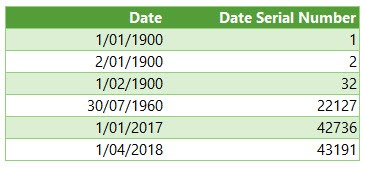
The Date Serial Number column displays the Date column values in their date serial number equivalent.

e.g. 1/1/2017 has a date serial number of 42736. i.e. 1^st January 2017 is 42,736 days since 31st December 1899.

Tip: format the date serial number column as a Date and you’ll see they look the same as the Date column values.

Time

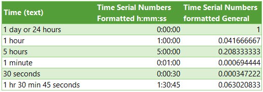
Times also use a serial number format and are represented as decimal fractions.

Hours: since 24 hours = 1 day, we can infer that 24 hours has a time serial number of 1, which can be formatted as time to display 24:00 or 12:00 AM or 0:00. Whereas 12 hours or the time 12:00 has a value of 0.50 because it is half of 24 hours or half of a day, and 1 hour is 0.41666′ because it’s 1/24 of a day.

Minutes: since 1 hour is 1/24 of a day, and 1 minute is 1/60 of an hour, we can also say that 1 minute is 1/1440 of a day, or its time serial number is 0.00069444′

Seconds: since a second is 1/60 of a minute, which is 1/60 of an hour, which is 1/24 of a day. We can also say one second is 1/86400 of a day or in time serial number form it’s 0.0000115740740740741…

Date & Time Together

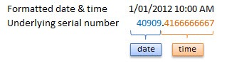
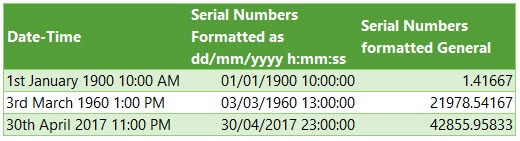
Now that we know how dates and times are stored we can put them together — ddddd.tttttt

For example, the date and time of 1^st January 2012 10:00:00 AM has a date-time serial value of 40909.4166666667

40909 being the serial value representing the date 1^st January 2012, and .4166666667 being the decimal value for the time 10:00 AM and 00 seconds.

More examples below.

Entering Dates & Times in Excel

Entering Dates

You can type in various configurations of a date and Excel will automatically recognise it as a date and upon pressing ENTER it will convert it to a date serial number and apply a date format on the cell.

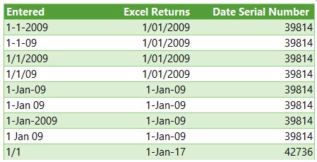
For example, try typing (or even copy and paste) the following dates into an empty cell:

1-1-2009

1-1-09

1/1/2009

1/1/09

1-Jan-09

1-Jan 09

1-Jan-2009

1 Jan 09

1/1

 

You can see in the table above that entering numbers that look like dates and are separated by a forward slash or hyphen will be recognised as a date. Even typing in a date with the month name gets converted to a date.

However, dates separated with a period like this 1.1.2009, or with spaces between numbers like this 01 01 2009, will end up as text, not a date. Gotta have some limits!

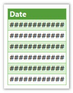
Tip: Dates that display ##### in a cell usually indicate that the column is simply not wide enough to display it.

However, if you make the cell really wide and it still displays ##### then this indicates that the date is a negative value and Excel can’t display negative dates.

Entering Dates with Two Digit Years

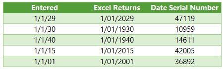
When you enter a date with two digits for the year e.g. 1/1/09, Excel has to decide if you mean 2009 or 1909.

It goes by the rule that dates with years 29 or before, are treated as 20xx and dates with the year 30 or older are treated as 19xx. See examples below.

Tip: You can enter the day and month portions of a date and Excel will insert the year based on your computer’s clock. Nice to know for data entry.

Entering Time

When you enter time you must follow a strict format of at least h:mm. i.e. the hour and minutes are separated by a colon with no spaces either side. Entering the h:mm components will result in a time formatted in military time e.g. 2:00 PM is 14:00 in military time.

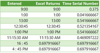
If you enter a time that includes a seconds component e.g. 3:15:40, Excel will automatically format the cell in h:mm:ss.

If you want the time to be formatted with AM/PM you can simply enter a space after the time and then type AM or PM, or apply the number format to the cell later. Here are some examples:

Entering Dates & Time Together

Now that we know how to enter dates and time separately we can put them together to enter a date and time in the same cell.

You can even enter time then date and Excel will fix the order for you.

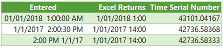
You’ll find that even if you enter AM/PM, that Excel will convert it to military time by default. You can override this with a custom number format. More on that later.

Simple Date & Time Math

Now that we understand that Excel stores dates and time as serial numbers, you’ll see how logical it is to perform math operations on these values. We’ll look at some simple examples here and tackle the more complex scenarios later when we look at Date and Time Functions.

Adding/Subtracting Days from Dates

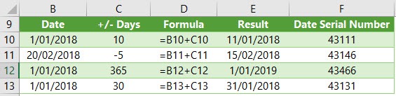
Tip: you can also add/subtract the days directly in the formula e.g. =B10+10 or =B11-5 Although, it’s better to place the values you’re adjusting by in their own cell or a named range.

Subtracting Dates from one another

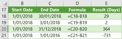
Tip: format the cell to General or Number to see the number of days between two dates.

Note: the ‘result’ is exclusive of the start day i.e. it assumes the start day is at the end of that day.

Adding Times to one another

The time being added is input as a time serial number. Notice there are no negative times in the table below. Remember we can’t display negative times. Instead we need to use the math operator to tell Excel to subtract time.  See examples below.

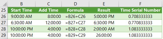
Note: Times that roll over to the next day result in a time-date serial number >= 1. Cell E28 actually contains a time-serial number of 1.08333′, but since the cell is formatted to display time formatted as h:mm:ss, only the time portion is visible.

If you want to show the cumulative time (like cell E29) then you need to surround the ‘h’ part of the time format in square brackets like so: [h]:mm:ss

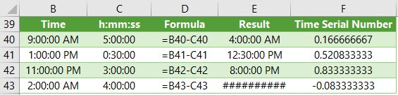
Subtracting Time from Times

Notice the last result in the table below shows ######, this is because it results in a negative time and Excel can’t display that, but notice it can return a negative time serial number. More on how to solve this later.

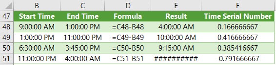
Subtracting Times from one another

Again, here the last result shows ###### because it results in a negative time.

Excel Date and Time Shortcuts

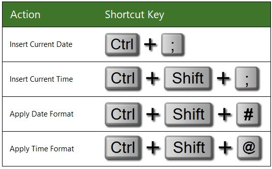
‘Good to Know’ Stuff about Excel Date and Time

— Dates prior to 1st January 1900 are not recognised in Excel.

— A negative date will display in the cell as #######

— Times stored without a date effectively inherit the date 0 Jan 1900 i.e. the month is Jan and the year 1900 and the day is zero. Remember, there are no dates prior to 1/1/1900 from Excel’s perspective. This means that times stored without a date e.g. 0.50 for 12:00 PM is the equivalent of 0 Jan 1900 12:00 PM.

This is important because if you try to take 14 hours from 12 hours (without a date) you’ll get the dreaded ###### display in the cell, because negative dates and times cannot be displayed. We’ll cover workarounds for this later, but for now keep in mind that math on dates and time that result in negative date-time serial numbers cannot be formatted as a date.

Date Modes

— Excel actually has two date modes. The other mode is called 1904 Date System and is used for compatibility with Excel 2008 for Mac and earlier Mac versions. You can change the date system in the Advanced Options.

In the 1904 date system dates are calculated using 1st January 1904 as the starting point. The difference between the two date systems is 1,462 days. This means that the serial number of a date in the 1900 date system is always 1,462 days greater than the serial number of the same date in the 1904 date system. 1,462 days is equal to four years and one day (including one leap day).

Caution; the date setting you choose applies to all dates within the workbook. You can’t mix and match modes and you shouldn’t reference workbooks that use a different date system in formulas.

Bottom line; don’t use the 1904 date system unless absolutely necessary! Click here for more on date systems in Excel.

— Excel applies date number formats based on your system region settings. For example, my system is set to display dates in dd/mm/yyyy format, but if you’re in the U.S. your system is likely to format them as mm/dd/yyyy. Excel will automatically convert the format of date serial numbers to suit your system settings as long as it’s one of the default date formats and not a custom number format.

More Excel Date and Time Tips

This post is just the beginning, the next steps in mastering Excel Date and Time are below:

• Every Excel Date and Time Function explained
• Formatting Date and Time in Excel
• Common Date and Time Calculations

Tip: Avoid waiting, download the workbook and get the above topics now.

There are many functions in Microsoft Excel that may be used to work with dates and timings in Excel. Each function completes a straightforward task, but by combining numerous functions into a single formula, you may handle trickier and more complicated problems. The purpose of discussing DATE functions in Excel is to help different people to perform more complex and challenging tasks by combining several functions within one formula.

The DATE function is used to calculate dates in Excel. Excel provides different functions to work with dates & times such as TODAY, NOW, WEEKDAY, EOMONTH, etc. which we will discuss here with examples.

1. DATE Function in Excel

It will return the date in serial number based on the year, month, or day value as provided.

Syntax:

DATE(year,month,day)

Arguments:

1. Year – This argument includes – 1 to 4-digit values. Excel understands this ‘year’ argument according to the date system of the local computer which we use. For example- Excel windows uses the 1900 date system by default which means DATE (21,2,6) gives the result as 06-02-1921.
2. Month – This argument includes a positive or negative integer that represents the month of the year from January to December.
3. Day – This argument also includes a positive or negative integer representing the day of the month from 1 to 31.

Excel Date Function Example 1:

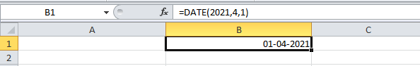
Excel Date Function Example 2:

 It will return on the first day of the current year & month.

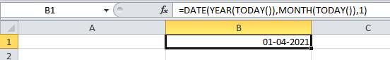
Excel Date Function Example 3:

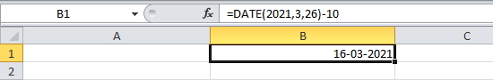
2. TODAY Function in Excel

The TODAY() function name suggests it will return today’s date, and it has no arguments.

Syntax: 

TODAY()

Example1: 

Here we will print the current date and also add 10 days to the current date.

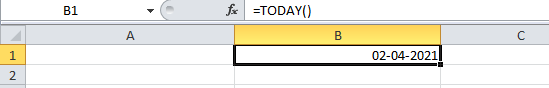
Example 2: 

To add 10 days to Today’s date.

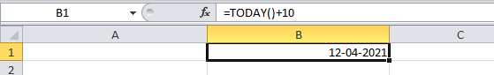
3. NOW Function in Excel

This function returns the current date as well as the time & doesn’t have any arguments.

Syntax: 

NOW()

Example:

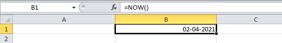
 4. DATEVALUE Function

It converts the date in text format to a serial number, which can be represented as a date.

Syntax: 

DATEVALUE(date_text)

Arguments:

1. date_text – This argument is a text that represents the date in Excel date format.

Example:

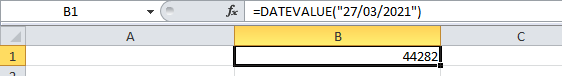
5. TEXT Function

It converts any numeric value not only dates to a text string. Through this function, we can change the date to text strings in a variety of formats.

Syntax: 

TEXT(value,format_text)

Arguments: 

1. value: The value that is to be converted.

2. format_text: The format in which you want to output the date value.

These are the different formats used in the TEXT function to change dates to text strings.

Example 1: 

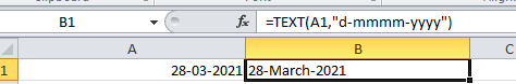
Example 2:

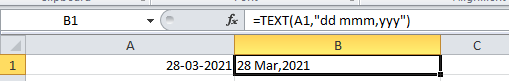
Example 3:

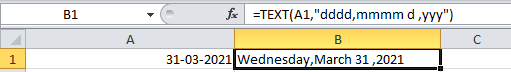
6. DAY Function

It returns the day of a month, i.e. integer from 1 to 31.

Syntax: 

DAY(serial_number)

Arguments:

1. serial_number: This value represents the day of the month you want to find. E.g: 5th day of June

Example 1:

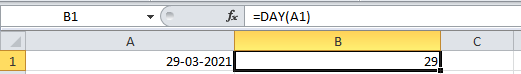
Example 2:

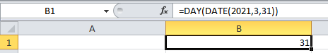
The DAY(TODAY()) function returns the day of today’s date, as shown below:

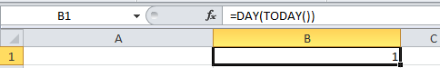
7. MONTH Function

This function returns the month of the given date as an integer from 1 to 12 (January to December).

Syntax: 

MONTH(serial_number)

Arguments: 

1. serial_number: This value represents the date for which you want to find the month.

Example:

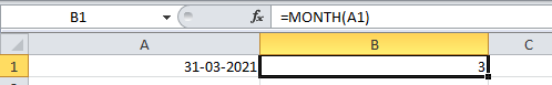
The MONTH(TODAY()) function returns the month of today’s date.

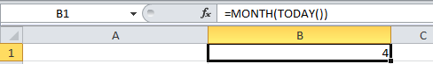
8. YEAR Function

It returns the year of a specified date.

Syntax: 

YEAR(serial_number)

Arguments:

1. serial_number: The date to be specified.

Example 1:

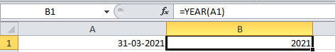
Example 2:

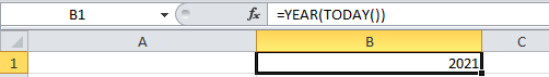
Example 3:

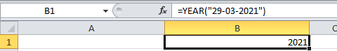
9. EOMONTH Function

This function returns the last day of the month after adding a specified number of months to a given date.

Syntax: 

EOMONTH(start_date,months)

Arguments:

1. start_date: In this argument, the date should be written in date format, not in the text.

2. months: In this argument, if a positive integer is given then corresponding months can be added to the start date & if a negative integer is given then the corresponding months can be subtracted from the start date.

Example 1:

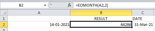
Example 2:

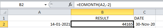
Example 3:

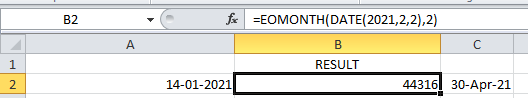
The EOMONTH(TODAY(),0) function returns the last day of the current month.

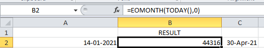
10. WEEKDAY Function

This function returns the day of the week as a number from 1 to 7 (Sunday to Saturday) according to the specified date.

Syntax: 

WEEKDAY(serial_number,return_type)

Arguments:

1. serial_number: It can be a date or the cell that contains the date.

2. return_type: It is optional, as it specifies which day should be considered as the first day of the week.

NOTE: 1st day of the week is by default Sunday.

Example 1:

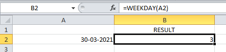
Example 2: 

In the below example, 2 is given as return_type i.e. Monday is referred to as the first day of the week.

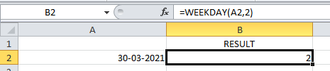
Example 3:

Here the day of today’s (01-04-2021) date is the result & the default value (Sunday) is considered here because no return_type is given.

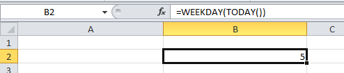
11. DATEDIF Function

This function calculates the difference between two dates in days, months, or years. For calculating the difference b/w dates which time interval should be used depends on the letter which we specify in our last argument i.e. at the unit.

Syntax: 

DATEDIF(start_date,end_date,unit)

Arguments:

1. start_date: The start date for evaluating the difference.

2. end_date: The end Date for evaluating the difference.

Example 1:

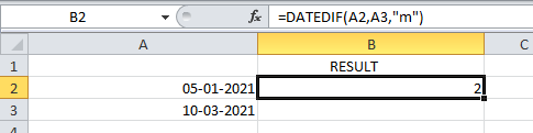
Example 2:

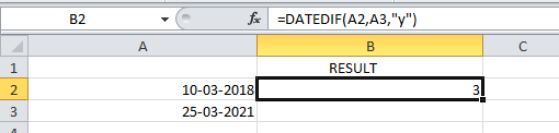
Example 3:

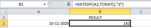
Here “m”,”y”,”d” means month, year & date. In the first example, the difference between dates is calculated by months, second by year & third by date.

12. WEEKNUM Function

It returns the week number based on the specified date, i.e. from 1 to 52 weeks of the year.

Syntax: 

WEEKNUM(serial_number,firstday_ofweek)

Arguments: 

1. serial_number: This is the date for which we want the week number.

2. firstday_ofweek: This is an optional argument that specifies which numbering system should be considered & which day of the week can be treated as the start of the week, Default(omitted) is 1. The table below is the parameters that can be given in firstday_ofweek argument.

First Day of the Week Start Table:

1	Sunday	1
2	Monday	1
11	Monday	1
12	Tuesday	1
13	Wednesday	1
14	Thursday	1
15	Friday	1
16	Saturday	1
17	Sunday	1
21	Monday	2

Example 1:

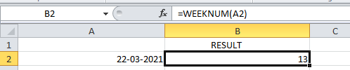
Example 2:

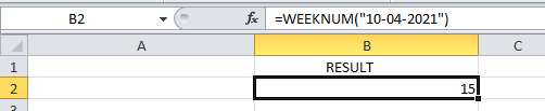
Example 3:

In the below example,21 is given as the second argument which means Monday is taken as the first day of the week & in the above example, the result shown is 15 but taking 21 as the first_dayofweek means Monday is the first day, the result is 14.

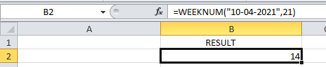
13. EDATE Function

This function adds or subtracts the specified month to a given date.

Syntax: 

EDATE(start_date,months)

Arguments:

1. start_date: This is an initial date on which the months are added or subtracted.

2. months: This is the number of months which is to be added or subtracted in the specified date.

Example 1:

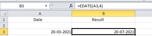
Example 2:

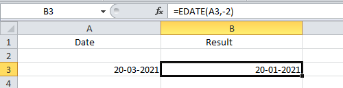
Example 3:

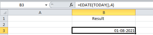
 14. YEARFRAC Function

This function returns the fraction of the year which represents the number of whole days between the start & end date.

Syntax: 

YEARFRAC(start_date,end_date,[basis])

Arguments:

1. start_date: This is the start date in the serial number.

2. end_date: This is the end date in the serial number.

3. basis: This is the optional argument that specifies the day count method.

Basis	Day count method
0(default)	US 30/360
1	actual/actual
2	actual/360
3	actual/365
4	European 30/360

Example 1: 

Using someday count methods.

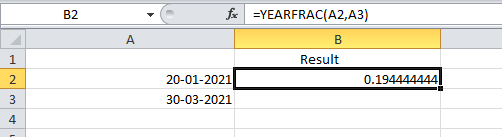
Example 2:

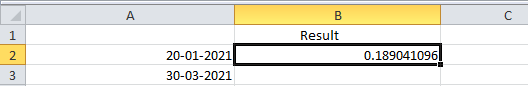
Example 3:

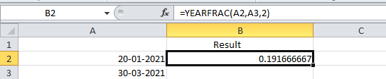
15. WORKDAY Function

This function helps if we exactly know how many working days we have & want to find out the date when the number of working will skip. This function always includes working days & excludes weekend days.

Syntax: 

WORKDAY(start_date,days,holidays)

Arguments:

1. start_date: This argument is the date from which the counting of weekdays begins. Excel doesn’t include start_date as a working day.

2. days: This is the number of working days.

3. holidays: This is an optional argument. If the days mentioned include any holidays, then we need to make a list of holidays separately for this, and mention it here.

Example 1: 

28 workdays from the start date, excluding holidays.

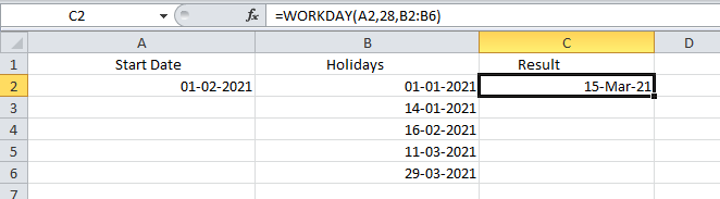
Example 2: 

28 workdays before the start date, excluding holidays

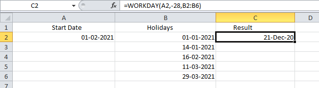
Example 3: 

28 workdays from the start date, no holidays.

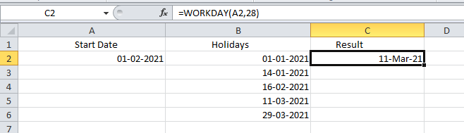
Example 4: 

28 workdays from today’s date, no holidays.

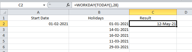
16. WORKDAY.INTL Function

This is a modification of the WORKDAY function as it provides a custom weekend parameter that distinguishes this from the WORKDAY function.

Syntax: 

WORKDAY.INTL(start_date,days,[weekends],holidays)

Arguments:

1. start_date: This argument is the date from which the counting of weekdays begins. Excel doesn’t include start_date as a working day.

2. days: This is the number of working days.

3. holidays: This is an optional argument. If the days mentioned include any holidays, then we need to make a list of holidays separately for this and mention it here.

4. weekends: Through this argument, we can specify which days of the week to be treated as non-working days, either by weekend number or specific character string.

Weekend Number:

Numbers	Days
1 (default)	Saturday, Sunday
2	Sunday, Monday
3	Monday, Tuesday
4	Tuesday, Wednesday
5	Wednesday, Thursday
6	Thursday, Friday
7	Friday, Saturday
11	Sunday
12	Monday
13	Tuesday
14	Wednesday
15	Thursday
16	Friday
17	Saturday

If this weekend argument is blank in this function, then it will automatically take the combination of Saturday & Sunday.

For instance:

• “0000011”-Saturday & Sunday are weekends(non-working days)
• “1000010”-Monday & Saturday are weekends(non-working days)

Example 1: 

30 days from the start date, excluding holidays & Sunday, and Monday as weekends (by giving weekend number 2 as arguments).

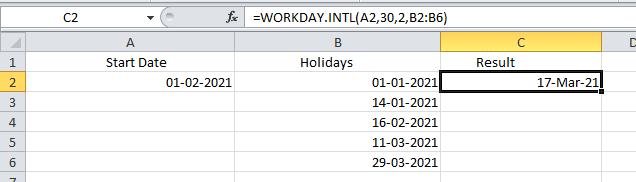
Example 2: 

30 days from the start date, excluding holidays & Sunday, Monday as weekends(by giving weekend string “1000001” as arguments).

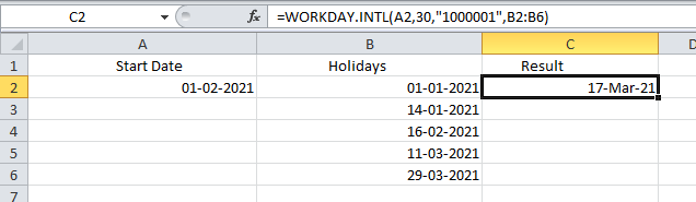
Example 3: 

20 days from the start date, no holidays & Monday, Saturday as weekends (by giving weekend string “1000010” as arguments).

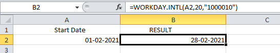
17. NETWORKDAYS Function

This function returns the number of working days between two dates, excluding weekends & holidays are as optional arguments.

Syntax: 

NETWORKDAYS(start_date,end_date,holidays)

Arguments:

1. start_date: The initial date to start evaluation.

2. end_date: The last date to end the evaluation.

4. holidays: Used to specify holidays.

Example 1:

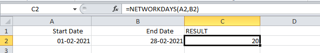
Example 2:

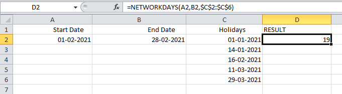
18. NETWORKDAYS.INTL Function

This function also returns the number of working days between two dates but provides the additional argument weekend to specify which days should be counted as weekend days.

The structure of the weekend argument is the same as for WORKDAY.INTL i.e. we can use either the weekend number or character string.

Syntax: 

NETWORKDAYS.INTL(start_date,end_date,[weekend],holidays)

Arguments:

1. start_date: The initial date to start the evaluation.

2. end_date: The last date to end the evaluation.

3. weekend: Use to specify the weekends.

4. holidays: Used to specify holidays.

Example 1: 

Here, the weekend argument is given in the form of a number.

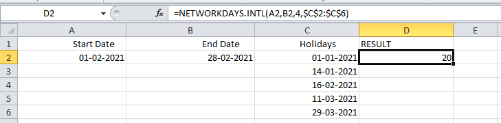
Example 2: 

Here, the weekend argument is given in the form of a character string of 0’s & 1’s.

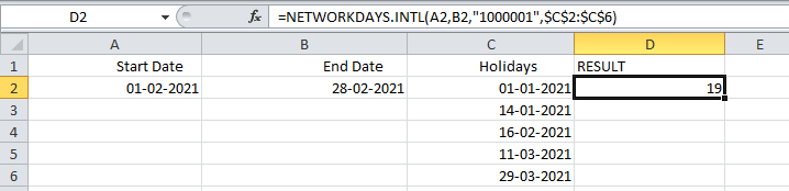
Hopefully, this extensive overview of Excel’s date functions has given you a general idea of how date formulas in Excel operate. I advise you to read more articles on Excel if you want to understand more. I appreciate your time and look forward to hearing from you soon!

FAQs on DATE Functions in Excel

Here are some of the most frequently asked questions on DATE Functions in Excel

1. What is a Date function?

The DATE function in Excel combines the three independent values of year, month, and day to create a date.

Syntax: DATE(year,month,day)

2. How do I get DD MMM YYYY in Excel?

• Pick the cell that contain the date>right-click and select Format Cells
• Select Custom in the Number Tab>type ‘dd-mmm-yyyy’ in the Type text box>click OK.