Date value to date in excel - Word и Excel - помощь в работе с программами

Excel for Microsoft 365 Excel for the web Excel 2021 Excel 2019 Excel 2016 Excel 2013 Excel 2010 Excel 2007 More…Less

Occasionally, dates may become formatted and stored in cells as text. For example, you may have entered a date in a cell that was formatted as text, or the data might have been imported or pasted from an external data source as text.

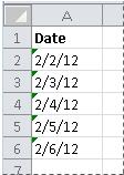
Dates that are formatted as text are left-aligned in a cell (instead of right-aligned). When Error Checking is enabled, text dates with two-digit years might also be marked with an error indicator: .

Because Error Checking in Excel can identify text-formatted dates with two-digit years, you can use the automatic correction options to convert them to date-formatted dates. You can use the DATEVALUE function to convert most other types of text dates to dates.

If you import data into Excel from another source, or if you enter dates with two-digit years into cells that were previously formatted as text, you may see a small green triangle in the upper-left corner of the cell. This error indicator tells you that the date is stored as text, as shown in this example.

You can use the Error Indicator to convert dates from text to date format.

Notes: First, ensure that Error Checking is enabled in Excel. To do that:

Click File > Options > Formulas.

In Excel 2007, click the Microsoft Office button , then click Excel Options > Formulas.
In Error Checking, check Enable background error checking. Any error that is found, will be marked with a triangle in the top-left corner of the cell.
Under Error checking rules, select Cells containing years represented as 2 digits.

Follow this procedure to convert the text-formatted date to a normal date:

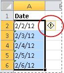
On the worksheet, select any single cell or range of adjacent cells that has an error indicator in the upper-left corner. For more information, see Select cells, ranges, rows, or columns on a worksheet.

Tip: To cancel a selection of cells, click any cell on the worksheet.
Click the error button that appears near the selected cell(s).
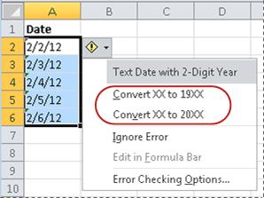
On the menu, click either Convert XX to 20XX or Convert XX to 19XX. If you want to dismiss the error indicator without converting the number, click Ignore Error.

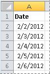
The text dates with two-digit years convert to standard dates with four-digit years.

Once you have converted the cells from text-formatted dates, you can change the way the dates appear in the cells by applying date formatting.

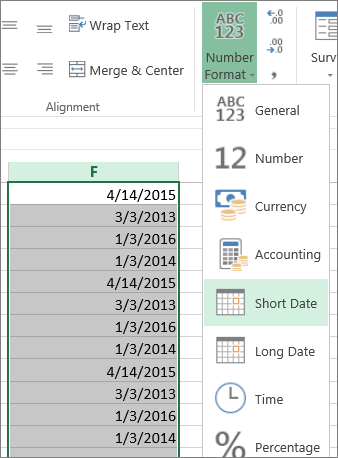
If your worksheet has dates that were perhaps imported or pasted that end up looking like a series of numbers like in the picture below, you probably would want to reformat them so they appear as either short or long dates. The date format will also be more useful if you want to filter, sort, or use it in date calculations.

Select the cell, cell range, or column that you want to reformat.
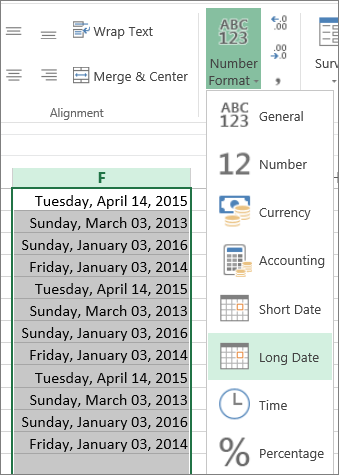
Click Number Format and pick the date format you want.

The Short Date format looks like this:

The Long Date includes more information like in this picture:

To convert a text date in a cell to a serial number, use the DATEVALUE function. Then copy the formula, select the cells that contain the text dates, and use Paste Special to apply a date format to them.

Follow these steps:

Select a blank cell and verify that its number format is General.
In the blank cell:
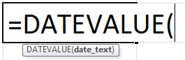
1. Enter =DATEVALUE(
2. Click the cell that contains the text-formatted date that you want to convert.
3. Enter )
4. Press ENTER, and the DATEVALUE function returns the serial number of the date that is represented by the text date.
  
  What is an Excel serial number?
  
  Excel stores dates as sequential serial numbers so that they can be used in calculations. By default, January 1, 1900, is serial number 1, and January 1, 2008, is serial number 39448 because it is 39,448 days after January 1, 1900.To copy the conversion formula into a range of contiguous cells, select the cell containing the formula that you entered, and then drag the fill handle across a range of empty cells that matches in size the range of cells that contain text dates.
After you drag the fill handle, you should have a range of cells with serial numbers that corresponds to the range of cells that contain text dates.
Select the cell or range of cells that contains the serial numbers, and then on the Home tab, in the Clipboard group, click Copy.

Keyboard shortcut: You can also press CTRL+C.
Select the cell or range of cells that contains the text dates, and then on the Home tab, in the Clipboard group, click the arrow below Paste, and then click Paste Special.
In the Paste Special dialog box, under Paste, select Values, and then click OK.
On the Home tab, click the popup window launcher next to Number.
In the Category box, click Date, and then click the date format that you want in the Type list.
To delete the serial numbers after all of the dates are converted successfully, select the cells that contain them, and then press DELETE.

Need more help?

You can always ask an expert in the Excel Tech Community or get support in the Answers community.

Need more help?

Want more options?

Explore subscription benefits, browse training courses, learn how to secure your device, and more.

Communities help you ask and answer questions, give feedback, and hear from experts with rich knowledge.

Источник

Purpose

Convert a date in text format to a valid date

Return value

A valid Excel time as a serial number

Usage notes

Sometimes, dates in Excel appear as text values that are not recognized as proper dates. The DATEVALUE function is meant to convert a date represented as a text string into a valid Excel date. Proper Excel dates are more useful than text dates since they can be formatted as a date, and directly manipulated with other formulas.

The DATEVALUE function takes just one argument, called date_text. If date_text is a cell address, the value of the cell must be text. If date_text is entered directly into the formula it must be enclosed in quotes.

Examples

To illustrate how the DATEVALUE function works, the formula below shows how the text «3/10/1975» is converted to the date serial number 27463 by DATEVALUE:

=DATEVALUE("3/10/1975")  // returns 27463

Note that DATEVALUE returns a serial number, 27463, which represents March 10, 1975 in Excel’s date system. A date number format must be applied to display this number as a date.

In the example shown, column B contains dates entered as text values, except for B15, which contains a valid date. The formula in C5, copied down, is:

=DATEVALUE(B5)

Column C shows the number returned by DATEVALUE, and column D shows the same number formatted as a date. Notice that Excel makes certain assumptions about missing day and year values. Missing days become the number 1, and the current year is used if there is no year value available.

Alternative formula

Notice that the DATEVALUE formula in C15 fails with a #VALUE! error, because cell B15 already contains a valid date. This is a limitation of the DATEVALUE function. If you have a mix of valid and invalid dates, you can try the simple formula below as an alternative:

=A1+0

The math operation of adding zero will cause Excel will try to coerce the value in A1 to a number. If Excel can parse the text into a proper date it will return a valid date serial number. If the date is already a valid Excel date (i.e. a serial number), adding zero will have no effect, and generate no error.

Notes

DATEVALUE will return a #VALUE error if date_text refers does not contain a date formatted as text.

Источник

Date yes Add (Subtract) Days to a Date Concatenate Dates Convert Date to Number Convert Date to Text Month Name to Number Create Date Range from Dates Day Number of Year Month Name from Date First Day of Month Add (Subtract) Weeks to a Date If Functions with Dates Max Date Number of Days Between Dates Number of Days in a Month Number of Weeks Between Dates Number of Years Between Dates Split Date & Time into Separate Cells Countdown Remaining Days Insert Dates Random Date Generator Using Dynamic Ranges — Year to Date Values Add (Subtract) Years to a Date Date Formula Examples Extract Day from Date Get Day Name from Date Count Days Left in Month / Year Count Workdays Left in Month / Year Get Last Day of Month Last Business Day of Month / Year Number of Work / Business Days in Month Weekday Abbreviations Auto Populate Dates Number of Months Between Dates Quarter from a Date Years of Service Change Date Format Compare Dates Time yes Add (Subtract) Hours to Time Add (Subtract) Minutes to Time Add (Subtract) Seconds to Time Add Up time (Total Time) Time Differences Change Time Format Convert Minutes to Hours Convert Time to Decimal Convert Time to Hours Convert Time to Minutes Convert Time to Seconds Military Time Round Time to Nearest 15 Minutes Overtime Calculator Number of Hours Between Times Convert Seconds to Minutes, Hours, or Time Count Hours Worked Time Differences Time Format — Show Minutes Seconds Text yes Add Commas to Cells Get First Word from Text Capitalize First Letter Clean & Format Phone #s Remove Extra Trailing / Leading Spaces Add Spaces to Cell Assign Number Value to Text Combine Cells with Comma Combine First and Last Names Convert Text String to Date Convert Text to Number Extract Text From Cell Get Last Word Remove Unwated Characters Extract Text Before or After Character How to Split Text String by Space, Comma, & More Remove Special Characters Remove First Characters from Left Substitute Multiple Values Switch First & Last Names w/ Commas Remove Specific Text from a Cell Extract Text Between Characters (Ex. Parenthesis) Add Leading Zeros to a Number Remove Line Breaks from Text Remove all Numbers from Text Reverse Text Remove Non-Numeric Characters Remove Last Character(s) From Right Separate First and Last Names Separate Text & Numbers Round yes Round Formulas Round Price to Nearest Dollar or Cent Round to Nearest 10, 100, or 1000 Round to Nearest 5 or .5 Round Percentages Round to Significant Figures Count yes Count Blank and Non-blank Cells Count Cells Between Two Numbers Count Cells not Equal to Count if Cells are in Range Count Times Word Appears in Cell Count Words in Cell Count Specific Characters in Column Count Total Number of Characters in Column Count Cells that Equal one of two Results Count Cells that do not Contain Count Cells that Contain Specific Text Count Unique Values in Range Countif — Multiple Criteria Count Total Number of Cells in Range Count Cells with Any Text Count Total Cells in a Table Lookup yes Two Dimensional VLOOKUP VLOOKUP Simple Example Vlookup — Multiple Matches Case Sensitive Lookup Case Sensitive VLOOKUP Sum if — VLOOKUP Case Sensitive Lookup Case Sensitive VLOOKUP Find Duplicates w/ VLOOKUP or MATCH INDEX MATCH MATCH Lookup — Return Cell Address (Not Value) Lookup Last Value in Column or Row Reverse VLOOKUP (Right to Left) Risk Score Bucket with VLOOKUP Sum with a VLOOKUP Function VLOOKUP & INDIRECT VLOOKUP Concatenate VLOOKUP Contains (Partial Match) 17 Reasons Why Your XLOOKUP is Not Working Double (Nested) XLOOKUP — Dynamic Columns IFERROR (& IFNA) XLOOKUP Lookup Min / Max Value Nested VLOOKUP Top 11 Alternatives to VLOOKUP (Updated 2022!) VLOOKUP – Dynamic Column Reference VLOOKUP – Fix #N/A Error VLOOKUP – Multiple Sheets at Once VLOOKUP & HLOOKUP Combined VLOOKUP & MATCH Combined VLOOKUP Between Worksheets or Spreadsheets VLOOKUP Duplicate Values VLOOKUP Letter Grades VLOOKUP Return Multiple Columns VLOOKUP Returns 0? Return Blank Instead VLOOKUP w/o #N/A Error XLOOKUP Multiple Sheets at Once XLOOKUP Between Worksheets or Spreadsheets XLOOKUP by Date XLOOKUP Duplicate Values XLOOKUP Multiple Criteria XLOOKUP Return Multiple Columns XLOOKUP Returns 0? Return Blank Instead XLOOKUP Text XLOOKUP with IF XLOOKUP With If Statement Misc. yes Sort Multiple Columns Use Cell Value in Formula Percentage Change Between Numbers Percentage Breakdown Rank Values Add Spaces to Cell CAGR Formula Average Time Decimal Part of Number Integer Part of a Number Compare Items in a List Dealing with NA() Errors Get Worksheet Name Wildcard Characters Hyperlink to Current Folder Compound Interest Formula Percentage Increase Create Random Groups Sort with the Small and Large Functions Non-volatile Function Alternatives Decrease a Number by a Percentage Calculate Percent Variance Profit Margin Calculator Convert Column Number to Letter Get Full Address of Named Range Insert File Name Insert Path Latitute / Longitude Functions Replace Negative Values Reverse List Range Convert State Name to Abbreviation Create Dynamic Hyperlinks Custom Sort List with Formula Data Validation — Custom Formulas Dynamic Sheet Reference (INDIRECT) Reference Cell in Another Sheet or Workbook Get Cell Value by Address Get Worksheet Name Increment Cell Reference List Sheet Names List Skipped Numbers in Sequence Return Address of Max Value in Range Search by Keywords Select Every Other (or Every nth) Row Basics yes Cell Reference Basics — A1, R1C1, 3d, etc. Add Up (Sum) Entire Column or Row Into to Dynamic Array Formulas Conversions yes Convert Time Zones Convert Celsius to Fahrenheit Convert Pounds to Kilograms Convert Time to Unix Time Convert Feet to Meters Convert Centimeters to Inches Convert Kilometers to Miles Convert Inches to Feet Convert Date to Julian Format Convert Column Letter to Number Tests yes Test if a Range Contains any Text Test if any Cell in Range is Number Test if a Cell Contains a Specific Value Test if Cell Contains Any Number Test if Cell Contains Specific Number Test if Cell is Number or Text If yes Percentile If Subtotal If Sumproduct If Large If and Small If Median If Concatentate If Max If Rank If TEXTJOIN If Sum yes Sum if — Begins With / Ends With Sum if — Month or Year to Date Sum if — By Year Sum if — Blank / Non-Blank Sum if — Horizontal Sum Count / Sum If — Cell Color INDIRECT Sum Sum If — Across Multiple Sheets Sum If — By Month Sum If — Cells Not Equal To Sum If — Not Blank Sum if — Between Values Sum If — Week Number Sum Text Sum if — By Category or Group Sum if — Cell Contains Specific Text (Wildcards) Sum if — Date Rnage Sum if — Dates Equal Sum if — Day of Week Sum if — Greater Than Sum if — Less Than Average yes Average Non-Zero Values Average If — Not Blank Average — Ignore 0 Average — Ignore Errors Math yes Multiplication Table Cube Roots nth Roots Square Numbers Square Roots Calculations yes Calculate a Ratio Calculate Age KILLLLLLL Calculate Loan Payments GPA Formula Calculate VAT Tax How to Grade Formulas Find yes Find a Number in a Column / Workbook Find Most Frequent Numbers Find Smallest n Values Find nth Occurance of Character in Text Find and Extract Number from String Find Earliest or Latest Date Based on Criteria Find First Cell with Any Value Find Last Row Find Last Row with Data Find Missing Values Find Largest n Values Most Frequent Number Conditional Formatting yes Conditional Format — Dates & Times Conditional Format — Highlight Blank Cells New Functions XLOOKUP Replaces VLOOKUP, HLOOKUP, and INDEX / MATCH Logical yes AND Checks whether all conditions are met. TRUE/FALSE IF If condition is met, do something, if not, do something else. IFERROR If result is an error then do something else. NOT Changes TRUE to FALSE and FALSE to TRUE. OR Checks whether any conditions are met. TRUE/FALSE XOR Checks whether one and only one condition is met. TRUE/FALSE Lookup & Reference yes FALSE The logical value: FALSE. TRUE The logical value: TRUE. ADDRESS Returns a cell address as text. AREAS Returns the number of areas in a reference. CHOOSE Chooses a value from a list based on it’s position number. COLUMN Returns the column number of a cell reference. COLUMNS Returns the number of columns in an array. HLOOKUP Lookup a value in the first row and return a value. HYPERLINK Creates a clickable link. INDEX Returns a value based on it’s column and row numbers. INDIRECT Creates a cell reference from text. LOOKUP Looks up values either horizontally or vertically. MATCH Searches for a value in a list and returns its position. OFFSET Creates a reference offset from a starting point. ROW Returns the row number of a cell reference. ROWS Returns the number of rows in an array. TRANSPOSE Flips the oriention of a range of cells. VLOOKUP Lookup a value in the first column and return a value. Date & Time yes DATE Returns a date from year, month, and day. DATEDIF Number of days, months or years between two dates. DATEVALUE Converts a date stored as text into a valid date DAY Returns the day as a number (1-31). DAYS Returns the number of days between two dates. DAYS360 Returns days between 2 dates in a 360 day year. EDATE Returns a date, n months away from a start date. EOMONTH Returns the last day of the month, n months away date. HOUR Returns the hour as a number (0-23). MINUTE Returns the minute as a number (0-59). MONTH Returns the month as a number (1-12). NETWORKDAYS Number of working days between 2 dates. NETWORKDAYS.INTL Working days between 2 dates, custom weekends. NOW Returns the current date and time. SECOND Returns the second as a number (0-59) TIME Returns the time from a hour, minute, and second. TIMEVALUE Converts a time stored as text into a valid time. TODAY Returns the current date. WEEKDAY Returns the day of the week as a number (1-7). WEEKNUM Returns the week number in a year (1-52). WORKDAY The date n working days from a date. WORKDAY.INTL The date n working days from a date, custom weekends. YEAR Returns the year. YEARFRAC Returns the fraction of a year between 2 dates. Engineering yes CONVERT Convert number from one unit to another. Financial yes FV Calculates the future value. PV Calculates the present value. NPER Calculates the total number of payment periods. PMT Calculates the payment amount. RATE Calculates the interest Rate. NPV Calculates the net present value. IRR The internal rate of return for a set of periodic CFs. XIRR The internal rate of return for a set of non-periodic CFs. PRICE Calculates the price of a bond. YIELD Calculates the bond yield. INTRATE The interest rate of a fully invested security. Information yes CELL Returns information about a cell. ERROR.TYPE Returns a value representing the cell error. ISBLANK Test if cell is blank. TRUE/FALSE ISERR Test if cell value is an error, ignores #N/A. TRUE/FALSE ISERROR Test if cell value is an error. TRUE/FALSE ISEVEN Test if cell value is even. TRUE/FALSE ISFORMULA Test if cell is a formula. TRUE/FALSE ISLOGICAL Test if cell is logical (TRUE or FALSE). TRUE/FALSE ISNA Test if cell value is #N/A. TRUE/FALSE ISNONTEXT Test if cell is not text (blank cells are not text). TRUE/FALSE ISNUMBER Test if cell is a number. TRUE/FALSE ISODD Test if cell value is odd. TRUE/FALSE ISREF Test if cell value is a reference. TRUE/FALSE ISTEXT Test if cell is text. TRUE/FALSE N Converts a value to a number. NA Returns the error: #N/A. TYPE Returns the type of value in a cell. Math yes ABS Calculates the absolute value of a number. AGGREGATE Define and perform calculations for a database or a list. CEILING Rounds a number up, to the nearest specified multiple. COS Returns the cosine of an angle. DEGREES Converts radians to degrees. DSUM Sums database records that meet certain criteria. EVEN Rounds to the nearest even integer. EXP Calculates the exponential value for a given number. FACT Returns the factorial. FLOOR Rounds a number down, to the nearest specified multiple. GCD Returns the greatest common divisor. INT Rounds a number down to the nearest integer. LCM Returns the least common multiple. LN Returns the natural logarithm of a number. LOG Returns the logarithm of a number to a specified base. LOG10 Returns the base-10 logarithm of a number. MOD Returns the remainder after dividing. MROUND Rounds a number to a specified multiple. ODD Rounds to the nearest odd integer. PI The value of PI. POWER Calculates a number raised to a power. PRODUCT Multiplies an array of numbers. QUOTIENT Returns the integer result of division. RADIANS Converts an angle into radians. RAND Calculates a random number between 0 and 1. RANDBETWEEN Calculates a random number between two numbers. ROUND Rounds a number to a specified number of digits. ROUNDDOWN Rounds a number down (towards zero). ROUNDUP Rounds a number up (away from zero). SIGN Returns the sign of a number. SIN Returns the sine of an angle. SQRT Calculates the square root of a number. SUBTOTAL Returns a summary statistic for a series of data. SUM Adds numbers together. SUMIF Sums numbers that meet a criteria. SUMIFS Sums numbers that meet multiple criteria. SUMPRODUCT Multiplies arrays of numbers and sums the resultant array. TAN Returns the tangent of an angle. TRUNC Truncates a number to a specific number of digits. Stats yes AVERAGE Averages numbers. AVERAGEA Averages numbers. Includes text & FALSE =0, TRUE =1. AVERAGEIF Averages numbers that meet a criteria. AVERAGEIFS Averages numbers that meet multiple criteria. CORREL Calculates the correlation of two series. COUNT Counts cells that contain a number. COUNTA Count cells that are non-blank. COUNTBLANK Counts cells that are blank. COUNTIF Counts cells that meet a criteria. COUNTIFS Counts cells that meet multiple criteria. FORECAST Predict future y-values from linear trend line. FREQUENCY Counts values that fall within specified ranges. GROWTH Calculates Y values based on exponential growth. INTERCEPT Calculates the Y intercept for a best-fit line. LARGE Returns the kth largest value. LINEST Returns statistics about a trendline. MAX Returns the largest number. MEDIAN Returns the median number. MIN Returns the smallest number. MODE Returns the most common number. PERCENTILE Returns the kth percentile. PERCENTILE.INC Returns the kth percentile. Where k is inclusive. PERCENTILE.EXC Returns the kth percentile. Where k is exclusive. QUARTILE Returns the specified quartile value. QUARTILE.INC Returns the specified quartile value. Inclusive. QUARTILE.EXC Returns the specified quartile value. Exclusive. RANK Rank of a number within a series. RANK.AVG Rank of a number within a series. Averages. RANK.EQ Rank of a number within a series. Top Rank. SLOPE Calculates the slope from linear regression. SMALL Returns the kth smallest value. STDEV Calculates the standard deviation. STDEV.P Calculates the SD of an entire population. STDEV.S Calculates the SD of a sample. STDEVP Calculates the SD of an entire population TREND Calculates Y values based on a trendline. Text yes CHAR Returns a character specified by a code. CLEAN Removes all non-printable characters. CODE Returns the numeric code for a character. CONCATENATE Combines text together. DOLLAR Converts a number to text in currency format. EXACT Test if cells are exactly equal. Case-sensitive. TRUE/FALSE FIND Locates position of text within a cell.Case-sensitive. LEFT Truncates text a number of characters from the left. LEN Counts number of characters in text. LOWER Converts text to lower case. MID Extracts text from the middle of a cell. PROPER Converts text to proper case. REPLACE Replaces text based on it’s location. REPT Repeats text a number of times. RIGHT Truncates text a number of characters from the right. SEARCH Locates position of text within a cell.Not Case-sensitive. SUBSTITUTE Finds and replaces text. Case-sensitive. TEXT Converts a value into text with a specific number format. TRIM Removes all extra spaces from text. UPPER Converts text to upper case. VALUE Converts a number stored as text into a number.

Источник

1) try using the DATEVALUE function and see if that works for you.

2) A more reliable way, since datevalue does not always work is to strip the text out manually and insert it into and excel date value. You are going to want to use a combination of the following functions:

DATE
TIME
IF
FIND
MID
LEFT
RIGHT
LEN

Now in my opinion the easiest way to do this is to work with multiple helper columns to build out all the steps. One column per step. When you get your final answer, you can substitute or copy paste your formulas from the helper columns into the final formula until you are left with one variable. The reason I say this is that the final formula referring to only 1 variable gets rather lengthy/ugly and very hard to trouble shoot if you make a typo, forget a bracket or something goes wrong. When I did this approach I used a totally of 14 columns (includes final formula). When I packed it all up into 1 formula it resulted in this:

DATE(RIGHT(LEFT(A3,FIND(" ",A3)-1),4),LEFT(LEFT(A3,FIND(" ",A3)-1),FIND("/",LEFT(A3,FIND(" ",A3)-1))-1),MID(LEFT(A3,FIND(" ",A3)-1),FIND("/",LEFT(A3,FIND(" ",A3)-1))+1,FIND("/",LEFT(A3,FIND(" ",A3)-1),FIND("/",LEFT(A3,FIND(" ",A3)-1))+1)-FIND("/",LEFT(A3,FIND(" ",A3)-1))-1))+TIME(LEFT(RIGHT(A3,LEN(A3)-FIND(" ",A3)),FIND(":",RIGHT(A3,LEN(A3)-FIND(" ",A3)))-1)+IF(AND(LEFT(RIGHT(A3,LEN(A3)-FIND(" ",A3)),FIND(":",RIGHT(A3,LEN(A3)-FIND(" ",A3)))-1)<12,RIGHT(RIGHT(A3,LEN(A3)-FIND(" ",A3)),2)="AM"),0,12),MID(RIGHT(A3,LEN(A3)-FIND(" ",A3)),FIND(":",RIGHT(A3,LEN(A3)-FIND(" ",A3)))+1,FIND(":",RIGHT(A3,LEN(A3)-FIND(" ",A3)),FIND(":",RIGHT(A3,LEN(A3)-FIND(" ",A3)))+1)-FIND(":",RIGHT(A3,LEN(A3)-FIND(" ",A3)))-1),MID(RIGHT(A3,LEN(A3)-FIND(" ",A3)),FIND(":",RIGHT(A3,LEN(A3)-FIND(" ",A3)),FIND(":",RIGHT(A3,LEN(A3)-FIND(" ",A3)))+1)+1,2))

Note it is set up using cell A3 as the one with the time as text that needs formatting.

3) You should also be able to use excel’s text to column function located on the DATA ribbon about half way across.

4) And of course there will be a way to code it through VBA as an option as well.

Источник

What does Excel DateValue Function do?

Excel DateValue function is used to convert a text to Date Serial, a numeric value that represents the Date.

Why do you need Excel DateValue Function?

Date is being treated specially in Excel. The format you see in Excel worksheet such as dd/mm/yyyy is only a displayed formatting, the underlying value of a Date is a numeric value. 1/1/1900 is considered as the first date in Excel, the numeric value of it is 1, and add one to each day onwards.

Everytime you do calculation on Date, Excel calculates using the numeric values. However if you actually type a Date in a condition or do a calculation, you need to enter the underlying numeric value instead of typing something like 1/1/2015.

For example, most people type a Date in A1 and A2 respectively to compare two Dates in Cell

=IF(A1>A2,”present”,”past”)

What really happening underneath is that Excel compares the two dates in numeric value, not comparing in “dd/mm/yyyy”. What if you need to actually type a Date in A2?

Should you type

=IF(A1>1/1/2015,"present","past")  OR

=IF(A1>"1/1/2015","present","past")  ??????

None of these will work, because you need the underlying numbers that represent the two dates, not a text, that is why DateValue Function is important, which transforms Date into numeric values.

Syntax of Excel DateValue Function

DATEVALUE( Date_text )

Date_text – a Date format with double quote, for example, “1/30/2008” or “30-Jan-2008”

After applying this formula, the function returns a date in Date Serial. You can change to display date format in Format Cells > Date.

Example of Excel DateValue Function

Formula	Result	Explanation
=DATEVALUE(“1/1/2015”)	42005	the 42005th days since 1/1/1900
=DATEVALUE(“1/1/2014”)	41640	the 41640th days since 1/1/1900
=DATEVALUE(“1/1/2015”)-DATEVALUE(“1/1/2014”)	365	42005-41640=365
=IF(A1>=DATEVALUE(“1/1/2015″),”future”,”past”)		Compare with Range A1
=IF(DATEVALUE(“1/1/2014”)>=DATEVALUE(“1/1/2015″),”future”,”past”)	past	41640 (1/1/2014) < 42005 (1/1/2015)

Outbound References

https://support.office.microsoft.com/en-in/article/DATEVALUE-function-4969e941-2edc-4292-89df-a82f02d14972?CorrelationId=f4debc2b-404c-4337-9579-dacb219aba9f&ui=en-US&rs=en-IN&ad=IN

Источник

Функция DATEVALUE (ДАТАЗНАЧ) в Excel используется для тех ситуаций, когда дата в ячейке указана в виде текста. С её помощью Excel конвертирует текстовое значение даты в число, которое система распознает как дату.

Содержание

Какие данные отображает
Синтаксис
Аргументы
Дополнительная информация
Примеры использования функции DATEVALUE (ДАТАЗНАЧ)
Пример №1. Преобразование даты в текстовом формате в число
Пример №2. Преобразование даты в текстовом формате с помощью формулы
Пример №3. Использование функции без указания года
Пример №4. Использование функции без указания дня

Какие данные отображает

Функция возвращает дату в виде числового значения, понятного по формату для Excel. Например, если мы используем функцию =DATEVALUE («1/1/2016») или =ДАТАЗНАЧ(«1/1/2016») , она будет возвращать число 42370, которое является числовым значением даты 01-01-2016.

Синтаксис

=DATEVALUE (“date_text”) — английская версия
=ДАТАЗНАЧ («дата_как_текст») — русская версия

Аргументы

date_text (дата_как_текст): это аргумент даты указанной в ячейке в формате текста или результат какой-либо формулы в виде текста;

для правильной работы функции, текст, который нам необходимо преобразовать в формулу важно указать в кавычках (прим. “01/01/2016”);
если date_text это результат какого-либо вычисления, важно чтобы ячейка была в текстовом формате, для корректной работы функции.

Дополнительная информация

DATEVALUE (ДАТАЗНАЧ) возвращает числовое значение даты:

Например: формула =DATEVALUE(“1/1/2014”) или =ДАТАЗНАЧ(“1/1/2014”) преобразует значение в число 41640, которое означает дату 1 января 2014 в формате даты.
Если вы указываете дату без дня (прим. =DATEVALUE(“1/2014”) или =ДАТАЗНАЧ(“1/1/2014”), а только месяц и год, система вернет числовое значение даты как первого дня указанного месяца — 41640, что для Excel будет означать как 01.01.2014.
Если вы не используете значение года (прим. =DATEVALUE(“01/04”) или =ДАТАЗНАЧ(“01/04”), Excel автоматически присвоит текущий год (указанный в настройках даты и времени вашей ОС).
Формат значения даты, которую выдает функция, зависит от настроек вашей ОС. Например в России (по умолчанию) при преобразовании даты 01/03/2016 это будет 1 Марта 2016, в США это 3 Января 2016.

Примеры использования функции DATEVALUE (ДАТАЗНАЧ)

Пример №1. Преобразование даты в текстовом формате в число

В приведенном выше примере, формула возвращает числовое значение даты введенной в кавычках. Введенная дата должна быть в текстовом формате, иначе Excel возвращает “#VALUE!” ошибку.

Обратите внимание, что значение, возвращаемое функцией зависит от настройки часов вашей системы. Если дата указана в формате ДД-ММ-ГГГГ значит «01-06-2016» будет отображать как 1 июня 2016 года, но для формата даты ММ-ДД-ГГГГ дата будет отображаться как 6 января 2016.

Больше лайфхаков в нашем Telegram Подписаться

Пример №2. Преобразование даты в текстовом формате с помощью формулы

Когда дата введена как текст в ячейку, вы можете использовать функцию DATAVALUE (ДАТАЗНАЧ), чтобы получить числовое значение даты. Обратите внимание, что дата должна быть в текстовом формате.

В приведенном выше примере, формула преобразует “1-6-16” и “1-июня-16” — это значение указанное в формате даты.

Эта функция полезна, когда у вас есть дата в текстовом формате, по которой вы хотите фильтровать, сортировать данные в таблице. В текстовом формате, вы не сможете сортировать даты и проводить вычисления в Excel, так как система будет рассматривать его как текст, а не число.

Пример №3. Использование функции без указания года

Если значение года не указано, то система использует текущий год при отображении значения даты (текущий год 2016 в указанном примере).

Пример №4. Использование функции без указания дня

Если в дате не указан день, то формула использует первый день месяца.

В приведенных выше примерах, когда мы вводим число «6-16», система возвращает число 42522, которое является значением даты на 1 июня 2016 года.

Источник

Let’s say you have an organization that makes hundreds of small transactions each day. You have several branches where the junior accountant punches in the numbers and dates into different software. It’s finally the end of the month, and you want to look at where you stand compared to the previous month.

This will require that you draw a gazillion charts, which is rather impossible to do unless you have a list of date-wise transactions. Since different branches may be using different programs, you will either need to import the data into an Excel file or type it in manually—you don’t have to be Einstein to make an instant choice here.

When you import data from databases, Excel may import those dates as text strings. The reason is, like Excel, not all programs store dates as serial numbers. When something is not a serial number, it’s not a date for Excel. This is why we are going to give you the rundown on some nifty formulas and methods that will help you create dates in your Excel worksheets.

How to Identify If Dates are Stored in Text?
3 Ways to Convert Dates Stored as Text
- Method 1 – Using DATEVALUE and VALUE Functions
- Method 2 – Using SUBSTITUTE + VALUE/DATEVALUE Function
- Method 3 – Using Text to Columns tool for Complex Text Strings
How and Why are Dates Stored as Numbers?
2 Ways to Convert Dates Stored as Numbers
- Method 1: Format Cells Dialog Box
- Method 2: Using the TEXT Function
How to Convert an 8-digit Date to an Excel-Recognizable Date
Fixing Text Dates with Two-Digit Years
- How to Enable/Disable Two-Digit Error Checking

How to Identify If Dates are Stored in Text?

When you try to use a certain list of dates with Excel tools like charts or PivotTables, they will fail to recognize data points as dates if they are stored as text. Although, there are several ways to just eyeball and determine if your list of dates are dates or text strings.

Alignment

Excel right-aligns dates by default. If your list of dates is leaning on the left wall of the cell, it may make a light bulb go off. Those are not dates, they are text strings.

Cell Format

The cell will be formatted as a “Date” in the Number Format box in Excel’s Home tab for data points that are recognized as dates by Excel.

Check the Status Bar

If you select the list of dates, you should see Average, Count, and SUM computed in the status bar, while you will see only Count if your dates are text strings.

3 Ways to Convert Dates Stored as Text

Let’s see some of the ways to convert dates stored as text to a date value that Excel can recognize.

Method 1 – Using DATEVALUE and VALUE Functions

DATEVALUE function is a catalyst that changes a date in text format into a serial number that Excel will identify as a date.

The formula has a single argument where you will input the text string:

=DATEVALUE(A2)

Instead of adding a cell reference, you could also add a text string manually.

If you get a random five-digit number after using the formula, don’t panic. This is not a random number, this is the serial number that Excel recognizes as a date. To view it as a date, navigate to the Number group in Excel’s Home tab and change the cell’s format to Date — this should fix your output.

While DATEVALUE works perfectly well, the VALUE function goes a step further to include time in its return. Excel stores dates as a serial number, and time as a decimal value after that serial number. For example, if the serial number for December 25, 2001, is 37250, then 37250.5 will represent December 25, 2015, 12:00 PM, since 0.5 would mean half a day.

VALUE function’s syntax is similar to that of the DATEVALUE function:

=VALUE(A2)

Notice how the output for the first two rows returns 12:00 AM even though no time has been inserted for those dates under the DATES column. This is because Excel reads this as an integer (naturally, since there is no decimal value), and therefore assumes the time as 12:00 AM, i.e. 0 hours into the returned date.

In the last row, we have entered 15:00 (i.e. 3 PM) as time. Notice how the VALUE function returns a serial number with a decimal value. If you want to manually compute time using this decimal value, just multiply it with 24 (0.625 * 24 = 15).

Method 2 – Using SUBSTITUTE + VALUE/DATEVALUE Function

VALUE function is a catalyst that changes a date in text format into a serial number that Excel will identify as a date.

In our example, we will use the VALUE function, but the formula will work the same way even if you choose to use the DATEVALUE function. The only difference being that the DATEVALUE function will not return the time component if any is present in your cells.

Let’s set up an example: we have a list of dates with a delimiter other than a forward slash (/) or a dash (-). Excel is currently reading the elements of this list as a text string. There are two ways to convert these text strings into a date. We have the following list of dates:

First, we could use the Replace tool in Excel to replace the delimiter.

Go to Home > Find & Select > Replace (Shortcut: Ctrl+H).

In the Find and Replace dialog box, enter a full stop (.) in the Find what text box, and a forward slash (/) in the Replace with text box. Down below, hit the Replace All (i.e. leftmost) button.

However, there is an easier way if you regularly populate your spreadsheet with new data — use a formula.

We know from our previous examples that the VALUE function is capable of converting text strings into a date. There is one caveat, though. Our text strings have a delimiter that keeps Excel from reading them as a date. So, we will need to supply a text string that has delimiters that Excel associates with a valid date.

Here’s the formula we will use:

=VALUE(SUBSTITUTE(A2, ".", "/"))

VALUE function does the same job here. It converts a text string into a date. We have nested a SUBSTITUTE function to deal with the delimiter issue. Had we directly referenced cell A2 inside the VALUE function, it would have returned a #VALUE! error since this text string cannot be recognized as a valid date in Excel.

All we need to do, then, is change the delimiter using the SUBSTITUTE function. Think of the SUBSTITUTE function as a formula for the Find & Replace tool we used in our previous example. It has 3 arguments: the first argument is a cell reference, the second argument is the character we want to replace, and the third argument is the character we want to replace with.

After executing the SUBSTITUTE function, our formula will look like this:

=VALUE("12/25/2001")

This should give us our final output, an Excel-recognizable date — 12/25/2001.

Method 3 – Using Text to Columns tool for Complex Text Strings

Last year, you made a terrible decision of hiring a sloppy manager who didn’t bother to create separate columns for the weekday and date. This has led you to pull your hair while trying to analyze your sales data.

Fret not, we will work together and see this problem through.

The sloppy employee has made entries like so:

Tuesday, December 25, 2001.

To convert these strings to dates, we will use a two-step process. Step 1 involves using an Excel tool called “Text to Columns,” and Step 2 involves using the DATE and MONTH function.

Step 1:

Select the list of text strings you wish to convert to dates.

Navigate to the Data Tools group under the Data tab and click on Text to Columns.

Choose Delimited in the dialog box that opens, and click Next.

On the next screen, you will choose the delimiters used in your text strings from the list. It is important to note that even space is considered a delimiter. Since our text strings have a space following the commas, we will check both delimiters on the list.
At the bottom of the dialog box, you will see a preview of how the text strings will be split after you click Next.

You have split the data, but there are still some miscellaneous things you need to run through. On the next screen, you will have the option to exclude any particular column from your output. For example, if the weekdays are irrelevant for you, exclude them by selecting the column (the column will turn black when selected), and choosing Do not import column (skip).

You may feel it is logical to choose Date under the Column data format list for the rest of the columns. However, remember that your text strings have been split into 3 components, and they cannot be recognized by Excel as a date. So, let them be formatted as General for now.

Finally, choose a destination where you want the return to be inserted, and click Finish.

Step 2:

We have our date split into three columns, and all we need to do now is bring them together and hand them over to Excel as a date. Although, there is still one loose end. Our month is a text string, while the DATE function needs a number.

To convert a month’s name to a number, we will nest the MONTH function inside the DATE function’s month argument. However, the MONTH function cannot work with just a text string, it needs a date so it can validly return the month number. We will circle back to this in a moment.

We will use this DATE formula:

=DATE(D2, MONTH(1&B2), C2)

If you are unfamiliar with the DATE function, take a quick tour of our DATE function tutorial.

The first and last arguments are just cell references to numbers that correspond to the year and date, respectively. So, what’s happening with the MONTH function?

Well, here’s what we are instructing the month function: Look at the value in D2 and give me the number from 1 to 12 for that month.

Had we only referenced the cell, the MONTH function could not have recognized the month. To remedy this, we concatenate a 1, which means it is now a date that the MONTH function can work with. 1 is just an arbitrary date, of course. You could have entered any number from 1 to 30/31 and it would still work.

So, we have now supplied the DATE function with all of its 3 arguments. This should give you a list of just the dates without the weekdays, and you can manipulate these dates in your worksheet as you see fit.

How and Why are Dates Stored as Numbers?

We know that Excel stores dates as serial numbers. Naturally, Excel does not just assign any random number to the dates; it follows a pattern. We will talk about this pattern in just a moment, but let’s first look at why Excel does this.

Why

There are several functions in Excel that manipulate the dates in the worksheet, including the DAYS, DATE, WORKDAY, DATEVALUE functions, among many others. These formulas need a standardized format that they can recognize as a date.

Consider that you are using the DAYS function, and have supplied two dates. You enter the end_date and the start_date and Excel computes the number of days to give you the output, i.e. the number of days between these dates.

In absence of serial numbers, Excel would have to use some alternate method to perform this computation. However, since Excel assigns a serial number, all it needs to do is subtract the two serial numbers and the resultant number will the number of days between these dates.

How

It is quite straightforward. Excel assigns ‘1’ to January 1, 1900. It adds 1 for each day from thereon. For example, January 2, 1900, will be assigned ‘2’.

January 1, 2021, is assigned 44197, which means 01/01/2021 occurs 44196 days after January 1, 1900.

This simplifies the computation and manipulation of dates to a great degree.

2 Ways to Convert Dates Stored as Numbers

We have some dates stored in our worksheet, but instead of being stored as dates, those cells have been formatted as General/Text/etc.

There are two ways we can convert these numbers to dates. Both instruct Excel to do the same thing, but in different ways.

Method 1: Format Cells Dialog Box

To convert the list of serial numbers to dates using this method:

Select the cells containing the values.
Navigate to the Number group under the Home tab in Excel.
Select Short Date or Long Date from the dropdown menu. This should convert the numbers to dates. However, if you want a custom format for your dates, continue to the next step.
Instead of opening the drop-down menu, click on the little arrow at the bottom-right of the Number group section. This should open up the Format Cells dialog box.
Select Date on the list that appears at the left of the dialog box.
You will see several date display formats listed in a box titled Type.

This will allow you to use a format of your choosing. However, if your desired format is not listed in the box, follow these steps:

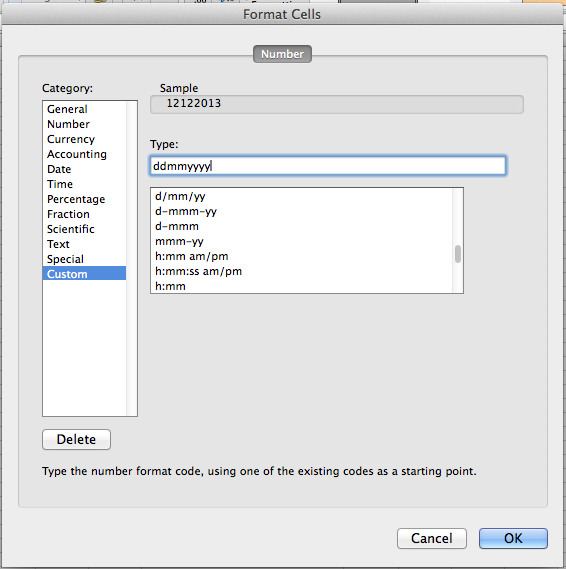
Instead of selecting Date from the list, select Custom. You will see several Custom formats listed in the box titled Type.
If you want to create a format on your own, use the following codes:

Code	Output
yyyy	Displays a 4-digit year: 1900-9999
yy	Displays a 2-digit year: 00-99
dddd	Displays weekdays: Sunday-Saturday
ddd	Displays 3-letter weekdays: Sun-Sat
dd	Displays the day component of the date, including 0: 01-31
d	Displays the day component of the date, excluding 0: 1-31
mmmmm	Displays the first letter of a month: J-D
mmmm	Displays the full month name: January-December
mmm	Displays the first three letters of a month: Jan-Dec
mm	Displays a number representing the month, including 0: 01-12
m	Displays a number representing the month, excluding 0: 1-12

These codes will also come in handy while applying Method 2. Speaking of which…

Method 2: Using the TEXT Function

This time around, we will use the TEXT function instead of manually formatting the cells.

The formula we will use is:

=TEXT(A2, "mm/dd/yyyy")

The formula does a very simple thing. It looks at cell A2 and applies the format “mm/dd/yyyy” to the text string in that cell.

It is essentially the same as what we did with the Format Cells dialog box, but with a formula. If you want a different format, refer to the table of codes above and adjust your formula accordingly.

How to Convert an 8-digit Date to an Excel-Recognizable Date

This is not a valid 5-digit serial number that Excel can recognize as a date. Therefore, we cannot directly change the cell’s format to convert it into a date. We will need an alternative method that involves parsing the text string and pulling its various components together using several functions to get our final output.

Here is the formula we will use:

=DATE(LEFT(A2, 4), MID(A2, 5, 2), RIGHT(A2, 2))

The DATE function will help us assemble the different components of a date via its year, month, and day arguments. These arguments all have different functions that will relay the information to them.

The LEFT, MID, and RIGHT function pick out the relevant component from the text string and relay that number to the DATE function. In our example, the LEFT function looks inside cell A2 and relays the first 4 characters of the text string contained in cell A2 as a year argument in the DATE function.

You can also use this formula if you have different delimiters in the text string separating the year, month, and day components of the date. All you need to do is adjust the character count in the LEFT, MID, and RIGHT functions.

Fixing Text Dates with Two-Digit Years

Unless you have entered a Custom format for any cell, a date that has a two-digit year will not sit well with Excel. Excel will add a green arrow at the top-left corner of each cell that has a date with a two-digit year.

To tackle this, hover your cursor over the cell. Doing this will bring up a drop-down button at the right of the cell with a yellow sign containing an exclamation mark. This sign tells you that there is an error, and you will see fixes (and other options) for the error in the dropdown menu.

The fixes will include two options, asking your preference regarding turning your dates into one that has a four-digit year. The first option will convert the year component into 19XX, the second will convert it to 20XX.

How to Enable/Disable Two-Digit Error Checking

If you do not see the error warning, you may have disabled error checking. You can enable/disable error checking by navigating to File > Options > Formulas and checking/unchecking the box besides the option that reads Enable background error checking.

You will also see specific Error checking rules down below. To get a warning for two-digit years, make sure you have checked the box besides the option that reads Cells containing years represented as 2 digits.

This takes care of almost all methods of converting text or numbers to date in Excel. Several other formulas could be used as alternative methods since Excel has a giant pool of powerful formulas, but the ones we discussed should help you sail through almost any date-conversion-related issues.

Drill these techniques by practicing them. By the time they become second nature to you, we will have some more formulas for you to explore.

Источник

The DATEVALUE function in Excel shows any given date in absolute format. This function takes an argument in the form of date text normally not represented by Excel as a date and converts it into a format that Excel can recognize as a date. This function helps make the given dates in a similar date format for calculations. The method to use this function is =DATEVALUE( date_text).

For example, if we insert “31Dec2021” as the text date, the DATEVALUE function in Excel would give us the result as “31/12/2021”

DATEVALUE Function in Excel
- Syntax
- How to use the DATEVALUE Function in Excel? (With Examples)
  - Example #1
  - Example #2
- Things to Remember
- Recommended Articles

Syntax

Arguments

date_text: A valid date in text format. The date_text argument can be entered directly or provided as a cell reference. If date_text is a cell reference, the cell value must be formatted as text. If date_text is entered directly, it should be enclosed in quotes. The date_text argument should only refer to the date between January 1, 1900, and December 31, 9999.
Return: It returns a serial number representing a particular date in Excel. It will produce a #VALUE! Error if date_text refers to a cell that does not contain a date formatted as text. If the input data is outside the range of Excel, the DATEVALUE in Excel will return #VALUE! Error.

How to use the DATEVALUE Function in Excel? (With Examples)

The Excel DATEVALUE function is very simple and easy to use. Let us understand the working of DATEVALUE in Excel by some examples.

You can download this DATEVALUE Function Excel Template here – DATEVALUE Function Excel Template

Example #1

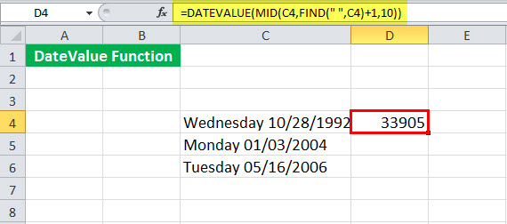
IIn this Excel DATEVALUE function example, suppose we have the day and date given in cell C4:C6. Now, we want to extract the date and get the serial number of the dates.

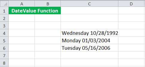
We can use the following Excel DATEVALUE function to extract the date for the first one and return the date value of the corresponding date:

= DATEVALUE ( MID (C4, FIND (” ” , C4) + 1, 10 ) )

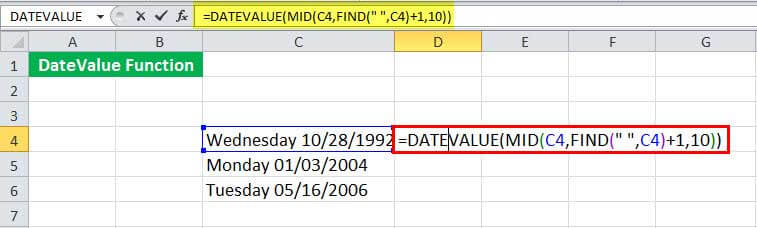
It will return the serial number for the date 28/10/1992.

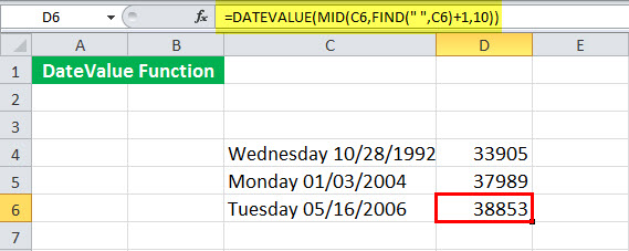
We need to drag it to the rest of the cells to get the date value for the remaining ones.

Now, let us see the DATEVALUE function in detail:

= DATEVALUE ( MID (C4, FIND (” “, C4) + 1, 10 ) )

FIND (” “, C4) will find the location of the 1st space occurring in cell C4.

It will return to 10.

FIND (” “, C4) + 1 will give the starting location of the date.
MID (C4, FIND (” “, C4) + 1, 10 ) will chop and return the cell text from the 10^th position to 10 places forward. For example, it will return on 28/10/1992.
DATEVALUE ( MID (C4, FIND (” ”, C4) + 1, 10 ) ) will finally convert the input date text to the serial number and return 33905.

Example #2

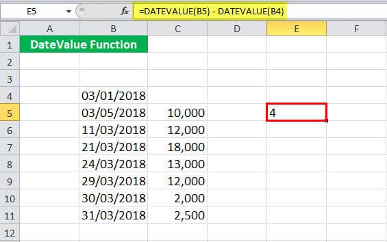
In this Excel DATEVALUE function example, suppose we have the data of sales collected at some time interval. The start date is 1 March 2018. Then, we collected the sales data on 5 March 2018. So, this represents the sales that have taken place between 1 and 5 March 2018. Next, we collected data on 11 March 2018, representing the sales between 5-11 March 2018.

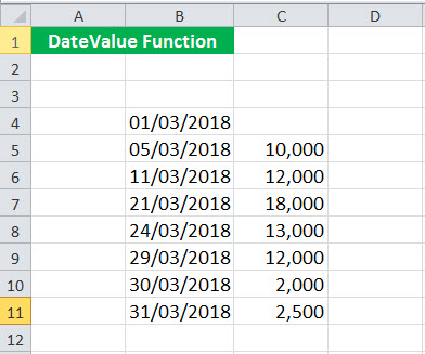
Now, we are not interested in the dates. Instead, we want to know how many days the sales were 10,000 (cell B5). To get the number of days, you could use the following DATEVALUE function:

= DATEVALUE (B5) – DATEVALUE (B4)

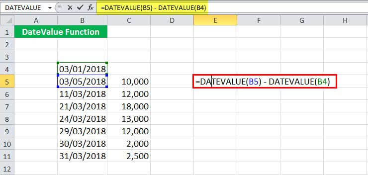
This DATEVALUE function in Excel will return 4.

We can now drag it to the rest of the cells.

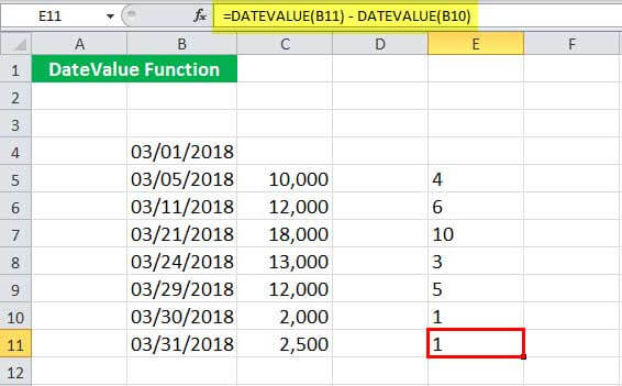
It is worth mentioning that with each day, the serial number of the date increases by 1. Since Excel recognizes the dates only after 1 Jan 1900, the serial number of this date is 1. For 2 Jan 1990, it is 2, and so on. Therefore, subtracting any two serial numbers will return the number of days between them.

Things to Remember

It converts any given date into a serial number, representing an Excel date.
If given a cell reference, the cell must be formatted as text.
This function will return a #VALUE! Error if date_text refers to a cell that does not contain a date or is not formatted as text.
It accepts a date only between January 1, 1900, and December 31, 9999.

Our Comment Policy.

We welcome your comments and questions about this lesson. We don’t welcome spam. Our readers get a lot of value out of the comments and answers on our lessons and spam hurts that experience. Our spam filter is pretty good at stopping bots from posting spam, and our admins are quick to delete spam that does get through. We know that bots don’t read messages like this, but there are people out there who manually post spam. I repeat — we delete all spam, and if we see repeated posts from a given IP address, we’ll block the IP address. So don’t waste your time, or ours. One other point to note — if you post a link in your comment, it will automatically be deleted.

Add a comment to this lesson

Comments on this lesson

amazing! solved my problem

amazing! solved my problem which i was battling for 2 days in office.

datevalue problem

hi there,

Very interesting solutions and it worked for one of my sheets. However, excel still returns the #VALUE! error message when I try to datevalue a date… Any other comments than the ones listed above?

Cheers,
Christian

datevalue problem

date looks somethink like «21-12-2011 10:45» I have the feeling that somthing goes wrong due to the hour and minute after the date. Any idea how to get rid of the time?

Date Format

Hi Chris

The DATEVALUE function is supposed to ignore time values. You’ll find that removing the time value from your example doesn’t solve the problem.

Question — can you confirm whether the quote marks are part of the value of the cell?

If they are, then they appear to be breaking the DATEVALUE function. I’m not sure why.

One solution you might consider is selecting just the date cells in your spreadsheet and doing a Find and Replace for the » character. By selecting only the cells you want, the Find/Replace will only operate on those cells. Removing the » character will convert the value into a date and you won’t need a formula to help you.

However, I also found that this formula would do the trick, assuming that you’ve got the quote symbol («) at the start and end of the date values you’re trying to convert:

=DATEVALUE(MID(A1,2,LEN(A1)-2))

This example assumes that the value I’m trying to convert to a date is in cell A1.

Essentially, the MID function takes the characters out from between the » characters, leaving you with just the raw date. The result is still considered by Excel to be a text value, though, so you need the DATEVALUE function as well.

David

Same problem

Chris,

I found that I used the text function mentioned above and did ok with this same formatting (database output) I used =—TEXT(LEFT(datecell, 5),»00000000″) Excel then took care of it after that for me.

Hope this helps and I’m not being redundant.

Dan

Hi,

Hi,
U can use the INT(Cell No)….as =INT(the cell u want to convert to date only)

EXCELL PROBLEM

HI I WANT TO KNOW HOW THIS FORMAT EX.13.10.2003 IS CONVERTED INTO 13TH OCT 2003
COULD U PLZ MAIL ME
THANK YOU
VIJAY

Converting text values into dates

Hi Vijay

If you have a value, 13.10.2003, in a cell, then Excel will see it as a text value rather than a numeric value. This is because there are two decimal points in the cell.

There are two ways to solve your problem of converting this text value into a date:

1. Use Excel’s Find and Replace feature.

This approach works well for a one-time conversion:

Select all the cells containing the dates you want to convert
Perform a Find and Replace where you search for «.» and replace it with «/».
This will instantly convert all of the values into valid dates.

2. Use DATEVALUE, LEFT, MID and RIGHT to convert a text string that looks like a date into an actual date

This option is more involved, and uses a version of Option Three in the lesson above to convert it to a date.

Let’s assume that you’ve typed this value, 13.10.2003, into A1, and then you want to convert it into a date using a formula in B1.

The formula you would enter in B1 is this:

=DATEVALUE(LEFT(A1,2)&»/»&MID(A1,4,2)&»/»&RIGHT(A1,4))

Here’s how this breaks down:

The LEFT function takes the first two characters in A1
The MID function takes two characters from the middle of A1, starting with the 4th character in A1
The RIGHT function takes the last two characters in A1
We use the & symbol to concatenate those values into a new text string.
The DATEVALUE function then converts that text string into a date.

The result is a value in B1 that contains a date. You can now use Excel’s date formatting tools to format it how you wish.

Note that this solution will only work on numbers in the specific format you supplied. It will not work if you want to convert a column of dates with values like this:

12.10.2003 — this will work with the formula supplied
13.10.2003 — this will work too
4.11.2004 — this won’t work. The LEFT function will retrieve «4.» instead of just 4, because it’s looking for two characters.
15.1.2004 — this won’t work either. The MID function will retrieve «1.» instead of just 1.

Note that it is possible to create a version of the formula I supplied that uses the FIND and LEN functions to figure out where the decimal points are, and how which characters to select in the LEFT, MID and RIGHT functions, although that function will end up being very long and complicated. Check out this comment below and my reply to see an example.

I hope that helps.

David

Thanks .. it really works

tnx.. perfect

hi there

i read the whole topic but that couldn’t solve my issue. i have a CSV with the date format like this «30.09.2013 09:36:14.213» I need to change it to «2013.09.30 09:36:14.213»
the custom format for it is gonna be «yyyy.mm.dd hh:mm:ss.ds»

do u have any idea ?

Combine functions and formatting to extract a date from text

Hi Arash

I love challenges like this. The answer is yes — it can be done. Here’s how:

Put the text date from your CSV into A1 in a new worksheet.
In A2, put this formula:
=DATEVALUE(LEFT(A1,2)&»/»&MID(A1,4,2)&»/»&MID(A1,FIND(» «,A1)-4,4))+RIGHT(A1,LEN(A1)-FIND(» «,A1))
The value in A1 is now a valid date in Excel.
Then, format the cell with a custom date format. Excel offers Date and Time functions as standard, but not a combined Date and Time function so we have to create our own:
- The Home tab in the toolbar has a Number section.
- Inside that is a drop-down option to choose from different number formats (the default is General).
- Choose Custom… to bring up the Number formatting dialog.
- Choose Custom from the Category list.
- In the Type box, replace what’s there with this: yyyy.mm.dd hh:mm:ss.000
The date value in A2 should now be formatted as a date plus time, like this: 2013.09.30 09:36:14.213.
Hopefully you can see how the value in cell A2 matches the custom format we applied in the previous step. In particular, note that the number of zeros at the end controls how many decimal places to show.

Here’s a quick explanation of the functions I used:

DATEVALUE takes a text value that looks like a date and turns it into a date.
LEFT takes the first x text characters from the start of a text value (the text in A1, in this case)
MID takes x characters from inside the string, once supplied with a starting point. The first time this formula uses it, it selects 2 characters starting at position 4 inside the string. The second time it’s used, FIND is used to determine the starting point.
The RIGHT function takes x characters starting from the end of the text string and working back. It needs to know how many characters to take, which is where the LEN and FIND functions.
The LEN function calculates the number of characters in the string of text.
FIND looks for the first instance of a character and returns its position inside the string. In this case, the formula uses FIND twice:
- inside a MID function to locate the first (and only) space and subtract 4 from that number. The MID function then selects 4 characters from that point, which gives us the year value.
- inside a RIGHT function, in combination with the LEN function, to determine how many characters to select. By finding the length of the text string with LEN, then subtracting the position of the space inside the text, we then know how many characters the RIGHT function should take.

I hope that helps!

David

hi david and tnx for the

hi david and tnx for the reply

i did what u told me but it give value error in A2. I copy the text date to A1 and copy paste the formula u provided into A2 when I press enter it gives value error.
is there any chance that I can send u the file itself so u can work on it directly ? it seems it is beyond my experience of excel

lemme know! tnx again

Problem with copy and paste

HI Arash

It’s possible the error was caused by some extra text being pasted into Excel. I found that when I posted it, I got this:

=DATEVALUE(LEFT(A1,2)&»/»&MID(A1,4,2)&»/»&MID(A1,FIND(» «,A1)-4,4))+RIGHT(A1,LEN(A1)-FIND(» «,A1)) — See more at: //fiveminutelessons.com/comment/415#comment-415

If you edit the cell and then remove everything after the last closing bracked, the formula should work OK. I’ve fixed this problem but it will take some time before the website reflects the fix. If that still doesn’t work, try manually typing the formula into the cell.

Regards

David

Try to replace the «,» (coma)

Try to replace the «,» (coma) with «;» in the formulas. This was the issue on my side.

@David,
I am glad I have found this place, as I am strugling with a report taken from CSV. As you rightly pointed out excel didn’t manage to recognize the date & tine in my case and actually no wonder as the dates given in the CSV are not perfectly formated.

These are the data I get form the CSV:
Column A: Received Column B: Resolved
A2: 5/22/2013 2:17:46 PM B2: 10/24/2013 11:52:57 AM

What I am trying to do is to convert the above text to date and time (preferably to 24h format if possible). I am stuch on this one now. I have trid to adopt your solutions but no luck so far — I will keep tryiong but meanwhile maybe you could help me out?

The next step will be to could the time tifference between the two cells, ie how many days/hours has passed since A2 to B2.

I would really appreciate your Help.
Thanks,
Robert

Is it a US date problem?

Hi Robert

I tried putting the two dates you supplied into a spreadsheet. The only issue I can see is that the dates are formatted for the US, i.e. month/day rather than day/month, which is the default format in my copy of Excel. Once I converted the dates to day/month format I was able to calculate the time between A2 and B2.

5/22/2013 2:17:46 PM becomes 22/5/2013 2:17:46 PM
10/24/2013 11:52:57 AM becomes 24/10/2013 11:52:57 AM

When subtracting A2 from B2 I get 154.89943287037, i.e. the number of days between them. Note that the value after the decimal point allows you to calculate the number of hours that have passed on the 155th day:

=MOD(B2-A2,1)*24

This formula returns a value of 21.5863888888853. It uses the MOD function to find only the value after the decimal point, and multiplies it to get the number of hours (it should be less than 24, since the value after the decimal point is a fraction of a day).

This brings me back to the original problem — what to do if you are importing a set of dates from a CSV or text file that are in a different format to the date formatting you are using.

The simplest way to do this is simply to change the date system in your version of Excel by changing the regional settings on your computer. You can then import the CSV file, after which you convert your computer back to your normal regional settings. Because Excel has imported the CSV and recognised the values as dates, it will now be storing the values as valid dates, and changing the regional settings back won’t affect them.

Let me know if this helps.

Regards

David

Hi David,

As usually the simplest ways usually work best! I did as you recomended, changed my regional settings to US, imported, converted from m-d-yyyy to d-m-yyyy and it works just great!!!

I did also notice that while importing data you ge to a point where you can define what a certain column will contain — one of the options gives date and it is possible to apply formatting. I havent checked that yet but I will soon.

Thank you very much for your help.

Rob

Excel’s import options didn’t work for me

Hi Rob

I considered that as a solution when answering your question but a quick test indicated that it wouldn’t work. I’d be interested to see if you have more luck than I did!

David

no difference

hi again

well… i noticed that sentence after bracket first time I copy paste the formula and removed it right away but still got value error. i manually typed it as well but no difference.
can u give me ur email address so I can send u the file ?

My date comes from an export

My date comes from an export that has «M/DD/YY» or «MM/DD/YY»

I am trying to get it into date so I can use the =weekday function.

Tried everything in this chain so far, to no avail. Any ideas?
dont know if this matters, but my computer I bought in Singapore and am now in the U.S. (i think my dates are in a diff format due to geographical difference)

Sorry, about the multiple

Sorry, about the multiple submits.

Can you help me? My dates are given in a mixture of numbers and characters. Could I use the DATAVALUE for this situation? Is there an alternative or even an easier way?

ex.
Fri Oct 25 23:59:59 CDT 2013
Thu Oct 24 23:59:59 CDT 2013
Wed Oct 23 23:59:59 CDT 2013
Tue Oct 22 23:59:59 CDT 2013
Mon Oct 21 23:59:59 CDT 2013

Trying to get 10/24/2013 11:52:57 AM into a Excel Date/Time

I am glad I have found this place, as I am strugling with a report taken from CSV. As you rightly pointed out excel didn’t manage to recognize the date & tine in my case and actually no wonder as the dates given in the CSV are not perfectly formated.

These are the data I get form the CSV:
Column A: Received Column B: Resolved
A2: 5/22/2013 2:17:46 PM B2: 10/24/2013 11:52:57 AM

The next step will be to could the time tifference between the two cells, ie how many days/hours has passed since A2 to B2.

I would really appreciate your Help.
Thanks,
Robert

Need help for data format conversion

I’ve a bunch of data that is format «280.605.890» which actually should have been a number «280605.890» . Do you have any idea how can I convert that data number in to the format I want? Please let me know, if you can help! Thanks!

Converting text to a number

Hi Shirish

If all numbers are in this format, i.e. xxx.yyy.zzz, then try this formula. Assume the number you want to convert is in cell A1:

=VALUE(LEFT(A1,3)&RIGHT(A1,6))

This will take the first three characters from the text string (the LEFT function does this), and the last 6 characters (the RIGHT function does this), and join them together in a new text string (this is called concatenation: the & symbol joins the result of the LEFT function to the result of the RIGHT function to create a new string). The VALUE function then converts the text value to a string (which it can do since the string is now a valid number).

If the number of digits in each group changes, you’d have to use the FIND function to work out where the first ‘.’ is, and use that result as the second argument in the LEFT function. The function would then look like this:

=VALUE(LEFT(A1,FIND(«.»,A1)-1)&RIGHT(A1,6))

In this case, the FIND function would determine that the ‘.’ is at position 4. We then have to subtract 1 to so the FIND function gets the characters up to but not including the ‘.’

From there, the only other complication I can see is the possibility that there are more than two decimal points inside the number. If that happens, you’d need to use the MID and LEN functions as well, to help identify the position of the additional decimal points. You can read more about the LEFT, RIGHT, FIND and MID functions here, and the LEN function here.

Date Format conversion

My database converted dates into Excel in this format: 12062013 and I need to convert that into a 12/06/2013 format. Suggestions?

Try Option Three in the lesson above

Hi Jodi

Assuming your dates are in month/day/year format, this formula will work (it assumes the date it’s converting is in A1):

=DATE(RIGHT(A1,4),LEFT(A1,2),MID(A1,3,2))

If your dates are in day/month/year format, try this instead:

=DATE(RIGHT(A1,4),MID(A1,3,2),LEFT(A1,2))

Both of these formulas assume the dates you’re working with are consistent, i.e. 2 characters + 2 characters +4 characters.

Regards

David

This is the formula I need

This is the formula I need with a slight difference. I have 110613 in cell H3 and when I used the formula, the year shows 2513. Please help!!

How to convert date to text

Hi, please show me how to convert date to text? I read your article about text to date, but my problem is the other way around. I need to convert 12/12/2013
to ‘20131212 thanks

Changing the format of an existing date

Hi Inga

If you are trying to change the way a valid date is presented, then you can simply change the format of the date. You need to select the cells and apply a custom date format that looks like this:

This examples shows the date example you gave with a custom format applied:

dd means show the day in 2 digits (so if the date was the 5th of December, it would appear as 05)
mm means show the month in 2 digits
yyyy means show the year in 4 digits.

Note that you could put this combination of dd, mm and yyyy in any order that you want, such as mmddyyyy. Excel will automatically use the underlying date value to show it correctly. You can also use any combination of other characters within the format, as shown in the two options directly below my custom format type in the example above.

Another thing worth noting is that you can use 1 letter, 2 letters, 3 letters or 4 letters. For example:

Using d will return 12, or 5 on the fifth
Using dd returns 12 or 05
Using ddd returns the first three letters of the day (Thu in your example)
Using dddd returns the full name of the day (Thursday)

This also works with the month value (m, mm, mmm, mmmm). It also works with the year value, but only yy (13) and yyyy (2013) are worth using.

This opens the potential for a date format such as this:

dddd, dd mmmm, yyyy
Thursday, 12 December, 2013

The great thing about this is it’s only a format, so the date stored in the cell doesn’t have to change in any way.

I hope this helps. Let me know if you still have any questions.

Regards

David

Microsoft Excel

I like the explaining method posted by expert. As I have been studying in Excel study but sometime it is very hard to get idea from the text book but you guys had made easier for us.

mixed column type

I need to convert a column to short date format. A few of the cells are already in date format, some cells are empty and if I put a 0 in them they convert to the date of 1/0/1900 showing that they are also in date format. But most cells have data looking like 11-15-2012. I’ve tried highlighting the column and highlighting individual cells and changing the number format, but nothing happens. I’ve tried the datevalue formula but get #VALUE instead. I’ve tried option 3 above on cell O9 with 11-15-2012 in it. [=DATE(LEFT(O9,2),MID(O9,4,2),RIGHT(O9,4))] gives me 9/2/1917. I can convert the text in cell O9 to a date if I double click in the cell, but I’ve got over 14,000 rows and I refuse to double click in all of them. Can you help me?

I thought maybe I had the

I thought maybe I had the equation wrong so I tried changing the equation to =DATE(RIGHT(O9,4),LEFT(O9,2),MID(O9, 3,2)) That gives me 10/30/2012. (How it got that out of 11-15-2012 I have no idea!)

Try the DATEVALUE function instead of DATE

Hi Beth

I can reproduce the scenarios you’ve described but I can’t explain them. The only thought that crossed my mind is that your example is in US date formats, whilst I’m using Excel with British date formats set on my computer, but that doesn’t seem to fit with the results we’re both getting.

However, I think I can solve the problem for you. Try this:

=DATEVALUE(LEFT(O9,2)&»/»&MID(O9,4,2)&»/»&RIGHT(O9,4))

The DATEVALUE function takes a text value and converts it to a date, provided the text string is presented as a valid date.

The formula I’ve supplied takes each date component from the value in O9 and concatenates them into a string where each date component is separated by a /

As I noted above, the date in O9 (11-15-2012), is in US date format (mm-dd-yyyy) whereas I’m using dd-mm-yy. So the formula given above doesn’t work for me — I have to swap the day and month components around. My version of that formula looks like this:

=DATEVALUE(MID(O9,4,2)»/»&LEFT(O9,2)&»/»&RIGHT(O9,4))

I hope that helps — let me know how you get on!

David

Convert text into number of months

I’m having trouble converting a series of cells that have time periods such as «1 year 8 months» or «3 months 2 weeks» into the number of months that contains. Can you help? Thanks

Convert Text to Date Issue

Hello! I hate to do this, but I read your document and comments section, which is very informative, but cannot seem to come up witha solution to my problem. I think my situation is unique, but not impossible. Who knows.

I have a fairly large doc full of data pulled from an export. The problem is there is a field for dates, and the system I guess put in the dates like this:

Mar 1 2011
Mar 10 2011

And I need to change these into an actual date format usable by Excel. I thought at first I could just use the Format Cells function, but I guess it cannot read this text as a date properly. I noticed, the data is a bit odd. Each entry has the abbreviated month, and then either one or two spaces after depending if the day of the month has one char or two. The other problem seems to be the abbreviated months.

Any thoughts on how I can quickly convert these dates?

Convert to Date Isue

Scott — did you get an answer for conversion question? I have the same issue with dates showing as SEP 2 2014 but I need to conver to 09/02/14.

Removing time from date

I’ve read through the article and comments but haven’t come across a solution. My CSV file has the dates written like this: April 1, 2010 3:04:12 PM EDT
I need to eliminate the timestamp completely. Trying to format the cells as just a date doesn’t work — it doesn’t change them to look like a date. It stubbornly refuses to change when I put the file in to XLS format.

I really need this timestamp to go away as it is interfering with my ability to import this data into another program.

Help please!

More data please…

Hi Rebecca

Can you give me some more examples to work with? I’ve got some ideas but need to make sure they’ll work on a range of different date values.

Regards

David

That’s the format all of the

That’s the format all of the dates are in. Interestingly enough when I delete the text in the cell and type in the date and time by hand it converts it to a number. When I select any cell the exact same format (in text form) shows in the formula bar. When I attempt to format the cell the display never changes. it’s like nothing every happened to the formatting.

I have over 2,000 records to import into my other program and it will NOT import the data if the timestamp remains in the cells. I’ll upload a sample XLS file so you can see what I mean.

Here’s a fix for your date problem

Hi Rebecca

Thanks for the additional data. For the readers who can’t see the file Rebecca sent me, it contained a column of dates that looked like this:

April 1, 2010 3:02:43 PM EDT
April 1, 2010 3:04:12 PM EDT
April 1, 2010 3:06:57 PM EDT
April 1, 2010 3:07:58 PM EDT
April 1, 2010 3:09:54 PM EDT
April 1, 2010 3:12:03 PM EDT
April 1, 2010 3:12:42 PM EDT
April 1, 2010 3:19:45 PM EDT
April 1, 2010 3:23:22 PM EDT
April 1, 2010 3:24:25 PM EDT
April 1, 2010 3:24:49 PM EDT

The challenge is to strip off the time and time zone values (e.g. 3:24:25 PM EDT) and convert what’s left into a valid date.

Here’s the formula to use, assuming the value to be converted into a date-only format is in A2:

=DATE(MID(A2,FIND(«, «,A2)+2,4),MONTH(DATEVALUE(LEFT(A2,FIND(» «,A2)-1)&» 1″)),MID(A2,FIND(» «,A2)+1,2))

This uses the DATE function as described in the main lesson body above, and then uses the FIND, MID and LEFT functions to pluck out the bits of the date we want.

If you’re trying to adapt this for your own use, you may need to tweak the FIND function. I’ve used the FIND function to identify where a specific pattern in the text appears so I can using that position to start the extraction of different pieces of the date.

The solution is complicated by the fact that Excel doesn’t know what to do with «April» inside the DATE function, so we use the MONTH function to convert April into 4, which Excel is then able to use in the DATE function.

I hope this helps — let me know if you have any further problems.

Regards

David

I am going crazy with numbers

Hi,

Please help with this 201312311834I1

I will separate it using «-» so we can better understand.. 2013-12-31-1834-I1

2013-12-31 — is the date and it should be 12/31/2013
1834 — This is the time and it should be 18:34
I1 — is null

I am really having a hard time to translate it to 12/31/2013 18:34

I have thousands of these in my report and it takes a lot of time to translate it to the correct format.

Please help me. Thanks

Combine the DATE and TIME functions to extract text

You could solve this using the following formula (assuming the time value to convert is in A1):

=DATE(LEFT(A1,4),MID(A1,5,2),MID(A1,7,2))+TIME(MID(A1,9,2),MID(A1,11,2),0)

This uses the DATE function as described in Option 3 in the lesson above and combines it with the TIME function which works in a very similar way to convert text into a time value. Since dates and times are just numbers in Excel, you are able to add them together to get a valid result.

Be warned that you’ll also need to apply a custom date format, otherwise the cell may only display the date and not the time. You can apply this custom date format to see both date and time in the cell at the same time:

d/mm/yy h:mm

Regards

David

Awesome

Column of dates

I have a column of dates that are in yyyymmdd format that need to be converted to mm/dd/yyyy format. How can I change the whole column?

Learner

Hi Cindy,

Follow below options to change the date format.

1. Select the cells that you want to change.

2. Click Data > Text to Columns, in the Convert Text to Columns Wizard, check Delimited, and click Next

3. In step2, directly click Next to continue.

4. In step 3, select Date from the Column data format, and choose YMD from the Date drop down list.

5. Then click Finish.

reply

Small Change…. in step3 select MDY

=NOW() formula

Hi All,

i have a problem in combining the 2 values in one cell…….

one cell contains name(example «Eranna») and other cell contains date(example «3/21/2014 5:09:26 PM»).

i need to combine both cells and my output should be «Eranna 3/21/2014 5:09:29 PM»

can anybody help me on this

You can combine these values using concatenation

Hi Eranna

You can combine two or more values into a single string of text using concatenation.

In your example, you could enter this formula:

=»Eranna «&»3/21/2014 5:09:26 PM»

Note how I put a space after Eranna before the closing quotation mark.

You could also write a formula like this:

=A1&» «&A2

This will take the value in A1 and combine with the value in A2. In my example I’ve also included a space between them (which I’ve put in quotation marks) but that part is optional.

I hope that helps.

Regards

David

combination

Hi David,

I had already tried to combine both values but it did not work.

below is the result.

Eranna 4/9/2014 13:50 PM = Eranna 41738.5765914352

output is not as I expected.

Regards,
Eranna.

You need to use the TEXT function when concatenating dates

Hi Eranna

It looks like it’s working, but Excel is removing the date formatting when concatenating the two values.

This formula will solve the problem for you:

=A1&» «&TEXT(A2,»mm/dd/yyyy hh:mm»)

Here’s a screenshot to help you visualise this:

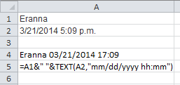
In this example, there is a text value in A1 and a date/time value in A1.

Using the TEXT function will convert the date value into a text string, which makes it appear correctly in the formula in A4.

Note how I have used &» «& within the formula to insert a space between the text value and the date.

I hope that solves the problem.

Regards

David

Absolutely ruddy brilliant,

Absolutely ruddy brilliant, thanks. Used the left right mid technique, spot on, cheers

Help!

I received data with the date formatted as: Tue, 7 Jan 2014 15:49:00

I need it to be formatted as 1/7/2014 in order to run a comparison in a database.

I need to reformat over 50,000 dates….

Any ideas??

Thank you for the post!

Hello,

Thank you for the detailed post, it was very informative as well as the comments and reply. I didn’t find a solution to my problem though. The date is in a APR-04-2014 and I would like it in a 4/4/2014 format. None of the formulas seem to be working.

Thanks for your help,
April

Convert date

I have this date formula like 06-APR-12 and I would like to have like this 06.04.2012.
Could you please help me?

If the cell is date format

If the cell is date format change it in what type of date format is convinient for you. If I presume that A1 cell is text format end contents «06-APR-12» then use in B1 cell formula =datevalue(A1) and the result will be 41005. Now format cell B1 date with the format that you wish. If you want to replace the content of A1 with B1 then from B1 copy to C1 paste value, delete B1 content and after that from C1 move to A1 and format A1 date with the format that you wish. Don’t forget to format B1 and C1 cell to general.

Thanks so much very helpful,

Convert a text value into a date in Excel

PLEASE HELP!!!

Hello,
I am trying to convert Tue Dec 10 12:37:13 PST 2013 to mm/dd/yy format and none of these techniques work. Am I doing something wrong?

Please help!

Thanks in advance,
Dimple.

Hi Dimple

Option 3 would have worked, but here’s a simpler solution, assuming your date is in A1:

=DATEVALUE(MID(A1,9,2)&» «&MID(A1,5,3)&» «&RIGHT(A1,4))

This formula takes the date (10), the month (Dec) and the year (2013) and combines them into a text string to look like this:

10 Dec 2013

It then applies the DATEVALUE to convert the resulting string into a date. This will yield a number rather than a date. Don’t worry — the number *is* the date:

41618

You can now use Excel’s date formatting options to format the date how you like (I provide more information on how to format dates in this comment: //fiveminutelessons.com/comment/658#comment-658)

Regards

David

I have a string of text

ES20140501-00722

I want to extract 20140501 and format it into a date (yyyy/mm/dd)

Please help..

Please help!

I have a string of text

ES20140501-00722

I want to extract 20140501 and format it into a date (yyyy/mm/dd)

Please help..

Hello Christabel,

Hello Christabel,
This is what I did:

Step 1: Extracted the month, date and year into individual cells using RIGHT, MID, LEFT formulas.
Step 2: Entered Month in text and their respective numerical values into a separate sheet (for instance, Jan 1, Feb 2, thru Dec 12 — «Jan» and «1» must be in individual cells, so on and so forth)
Step 3: Used VLOOKUP in to the first sheet (referencing the second sheet mentioned in step 2) to convert the months into their respective numerical value.
Step 4: Used CONCATENATE into a final column using the information from Step 1 and Step 3.

Hope this helps.

Dimple.

This earlier comment has another solution

Hi Christabel

Dimple’s solution will work (thanks Dimple!).

You could also check out this earlier comment which has another approach

Regards

David

Hi

I would like assistance in converting the following text «16-MAY-14 02.39.28.000000 AM» into the following format: DD:MM:YY 14:39

Converting Saturday, July 12, 2014 10:53 PM TO 12-Jul-14

Please help me convert Saturday, July 12, 2014 10:53 PM TO 12-Jul-14

Excel Date

I really appreciate your efforts…thanks.

Not working

This is great, however my problem is more complex. I have thousands of dates and not enough time to clean them! They are in the formats 1/02/2014 and 01/02/2014 and 1/2/2014 and just can’t be read in as dates (grrr!)

The RIGHT, MID and LEFT functions are not that helpful as I will then need to look at each one individually. I might as well just retype the date. How do i force it to read the day before the first / and so on?

Well I solved this one. If

Well I solved this one. If anyone needs it; I wrote nested ISERROR commands for each variation (2 digits behind the first slash, 1 digit, etc). If a slash goes into a date it returns an error so it checks the next option until it finds the right one.

Then for the random ones with odd variations I used conditional formatting to find them and fixed them manually (beats checking them all!)

ROW does not use dd-mm-yyyy, ISO is YYYY-MM-DD

Convert text date to functional date

Excellent. Thank you very much — it worked perfectly in no time at all.

convert general format to date format

Hi there, I have dates which looks like 08-10-12 (dd-mm-yy) which is written in general format. when i convert it to date format it changes day to month, which means instead of showing the month of october it shows august for the above given date, how can i solve this problem to convert thousands of such dates from general to date format???

I’m having difficulty

I’m having difficulty converting a text cell with 141217 into a date that reads 12/17/2014. Can anyone help?

Thanks!

Thanks =D

I just felt the need to say thanks because this really helped me out, it was very nicely written and with little to no effort I learned even more than what I came for, which is just great!! =D

i have this for my date 26 03

i have this for my date 26 03 where ddmm. how do i convert this to Mar 26?

Thanks a lot for those great

Thanks a lot for those great explanations! Problem solved! :o)

Date-Time formatting

Good Afternoon,

I am trying to separate the date and time in my excel worksheet. The data was imported from another database and so it is showing in text format.

the date and time shows as follows:
08/25/2014 — 05:23

I tried using the formula =—TEXT(LEFT(A3,5),»000000000″) but the value that is being returned is 08/25/2015. It doesn’t matter if I change the year in the original data, the returning data is always 2015. I don’t understand what step I am missing.

Please help,

Thank you,
Arzina

Combineing date and time while still having «date/time» format

Hello. I am trying to combine a «date column» with a «time column» so i have my data on the format: YYYY-MM-DD hh:mm:ss and it not being a text format. The reason for this is that in my next step i want to subtract 1h from the date/time column i have created, which wont work if it has a text format and unless they aren’t combined i cant subtract time to my knowledge.

i am having the date format

i am having the date format as

Mon May 5 16:48:55 2014
Wed Jul 2 20:09:40 2014
Mon Jun 15 18:38:50 2015
Mon Jun 15 18:38:50 2015
Fri Nov 29 01:14:53 2013
Fri Nov 29 01:18:24 2013
Fri Sep 19 00:33:25 2014
Mon Apr 13 00:24:22 2015

how can i convert this to normal date format which can be more effective for sorting out the latest date

Convert a text value into a date in Excel — Thanks, good tips

Just wanted to say thanks for a good, clear set of tips. Had to break out the big guns (parse the text and recombine to get a value) but it worked.

Convert 6 or 8 numbers to date format without helper cells

I want to convert a series of 6 or 8 numbers into date format automatically.
Example:

Column F2
Birthday
063055—————> I want that converted to 06/30/1955 in the same cell.
or
06301955————> converted to 06/30/1955 in the same cell.

Help.

Removing variable text from a data cell

I have an unknown combination of data that will be entered into a cell that I want to strip out if it is there. For example:

(DE) Smith, John
( DE) Smith, John
( DE )Smith, John
DE Smith, John

I will always want to remove the following values (, DE, and ) if they exist in the cell, but want to keep the Smith, John. I’ve used the following formula
=RIGHT(C21,LEN(C21)-FIND(«)»,C21))
This works great when there is a closing ), but in some cases the cell won’t have the closing ) — such as my last example above. Is there a way to accommodate for the removal of any combination of the examples above while still leaving the rest of the person’s name in this case?

What happens when DATEVALUE doesn’t work?

A common problem experienced in Excel and this article succinctly covered the possible issues and solutions.
Spot on! Thank you.

CONVERTING TEXT EXPORTED FROM OUR SYSTEMS

WHEN WE EXPORT THE TIME STAMP FROM OUR SYSTEMS, WE GET THE FOLLOWING NUMBER: EXAMPLE:20150903132429

THE FIRST PART IS THE DATE 20150903, WHICH I NEED CONVERTED TO 2015/09/03
THE SECOND PART IS THE TIME STAMP 132429. WHICH IN NEED CONVERTED TO 01:24:29

HOW WOULD I GO ABOUT DOING THIS TASK? AND, CAN I HAVE BOTH DATA AND TIME CONVERTED INTO THE SAME CELL?

re: CONVERTING TEXT EXPORTED FROM OUR SYSTEMS

Hi George,

assuming your example value is in cell A1, a way to get the value your system exported into a date and time format for excel is as follows:
=DATE(MID(A1,1,4),MID(A1,5,2),MID(A1,7,2))+TIME(MID(A1,9,2),MID(A1,11,2),MID(A1,13,2))
formatting said value into yyyy/mm/dd and hh:mm:ss can be done with the ribbon [number format]/[custom] and entering «yyyy/mm/dd hh:mm:ss» without quotes in the type field.
This of course will make your time format a 24 hour format (13:24:29) unless you add am/pm to the format, then it will display (01:24:29 PM) — like below…

Or you can display it as a text with:
=TEXT(DATE(MID(A1,1,4),MID(A1,5,2),MID(A1,7,2))+TIME(MID(A1,9,2),MID(A1,11,2),MID(A1,13,2)),»yyyy/mm/dd hh:mm:ss AM/PM»)

HTH

Excellent numbers to text, to dates guidance

Hi Team,

Thank you for posting a well written and helpful article, which assists me greatly in the current analytics work I’m doing. You can also see the completed works in LinkedIn. Thanks.

Chris Lira

Excel Question

I am exporting data from a database which formats a date in the following manner:
Sep 11 2015 1:50PM
but I need to convert it to the following format to import into another database:
09/11/15 or 091115

Is there a formula I can use to automate this converting? As I’m importing hundreds of line items with varying dates I am not versed well enough in Excel to figure out a better way to do this than manually replacing.

Any help would be greatly appreciated!

Thanks

Complicated data extraction

I am trying to convert a messy table to an excel spreadsheet for importing into a wordpress site.

I have attached a copy of the data as an example

I need to do a few things:
1) Extract the surname into its own cell
2) Extract the first name into its own cell
3) Extract address from second cell
4) Remove date
5) Remove registered
6) Remove ‘civil ceremonies’
7) Extract phone number
Extract suburb and state to own cell

I don’t know if this is remotely possible but would appreciate the help

converted dates

I need converted dates into Excel in this format: 811101-07-5429 and I need to convert that into a 01/11/1981 format. Suggestions?

Date in Text Format..

I Have dates which is in General Format and look like

Jun 19 2006
Jan 23 1995
Mar 11 2003
Jan 05 2007
Dec 15 1981
Jan 23 2009
Sep 11 1987

Can anyone suggest how to change these dates in «dd/mmm/yyyy» format..

Thanks..

Kundanlal

CREATING EXCEL FORMULAS

I WOULD BE GRATEFUL TO KNOW HOW TO CREAT EXCELL FORMULA TO FIND DATE OF DELIVERY FROM THE DATE OF PURCHASE ORDER IN BOTH MONTH AND WEEKS. E.G.

PO DATE : 05-01-2022
DELIVERY PERIOD IS : 3.5 MONTHS (3 MONTHS + 2 WEEKS),
WHAT IS THE FORMULA FOR THE ABOVE.

WARM REGARDS,
EDWARD

Источник

Need more help?

Need more help?

Want more options?

Purpose

Return value

Usage notes

Examples

Alternative formula

Notes

What does Excel DateValue Function do?

Why do you need Excel DateValue Function?

Syntax of Excel DateValue Function

Example of Excel DateValue Function

Outbound References

Какие данные отображает

Синтаксис

Аргументы

Дополнительная информация

Примеры использования функции DATEVALUE (ДАТАЗНАЧ)

Пример №1. Преобразование даты в текстовом формате в число

Пример №2. Преобразование даты в текстовом формате с помощью формулы

Пример №3. Использование функции без указания года

Пример №4. Использование функции без указания дня

How to Identify If Dates are Stored in Text?

3 Ways to Convert Dates Stored as Text

Method 1 – Using DATEVALUE and VALUE Functions

Method 2 – Using SUBSTITUTE + VALUE/DATEVALUE Function

Method 3 – Using Text to Columns tool for Complex Text Strings

How and Why are Dates Stored as Numbers?

2 Ways to Convert Dates Stored as Numbers

Method 1: Format Cells Dialog Box

Method 2: Using the TEXT Function

How to Convert an 8-digit Date to an Excel-Recognizable Date

Fixing Text Dates with Two-Digit Years

How to Enable/Disable Two-Digit Error Checking

Table of contents

Syntax

How to use the DATEVALUE Function in Excel? (With Examples)

Example #1

Example #2

Things to Remember

Recommended Articles

Our Comment Policy.

Comments on this lesson

1. Use Excel’s Find and Replace feature.

2. Use DATEVALUE, LEFT, MID and RIGHT to convert a text string that looks like a date into an actual date