
Excel for Microsoft 365 Excel for the web Excel 2021 Excel 2019 Excel 2016 Excel 2013 Excel 2010 Excel 2007 More…Less
Occasionally, dates may become formatted and stored in cells as text. For example, you may have entered a date in a cell that was formatted as text, or the data might have been imported or pasted from an external data source as text.
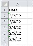
Dates that are formatted as text are left-aligned in a cell (instead of right-aligned). When Error Checking is enabled, text dates with two-digit years might also be marked with an error indicator:  .
.
Because Error Checking in Excel can identify text-formatted dates with two-digit years, you can use the automatic correction options to convert them to date-formatted dates. You can use the DATEVALUE function to convert most other types of text dates to dates.
If you import data into Excel from another source, or if you enter dates with two-digit years into cells that were previously formatted as text, you may see a small green triangle in the upper-left corner of the cell. This error indicator tells you that the date is stored as text, as shown in this example.
You can use the Error Indicator to convert dates from text to date format.
Notes: First, ensure that Error Checking is enabled in Excel. To do that:
-
Click File > Options > Formulas.
In Excel 2007, click the Microsoft Office button
 , then click Excel Options > Formulas.
 -
In Error Checking, check Enable background error checking. Any error that is found, will be marked with a triangle in the top-left corner of the cell.
-
Under Error checking rules, select Cells containing years represented as 2 digits.
 , then click Excel Options > Formulas.
Follow this procedure to convert the text-formatted date to a normal date:
-
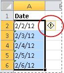
On the worksheet, select any single cell or range of adjacent cells that has an error indicator in the upper-left corner. For more information, see Select cells, ranges, rows, or columns on a worksheet.
Tip: To cancel a selection of cells, click any cell on the worksheet.
-
Click the error button that appears near the selected cell(s).
-
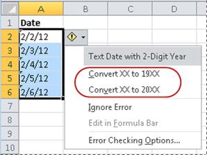
On the menu, click either Convert XX to 20XX or Convert XX to 19XX. If you want to dismiss the error indicator without converting the number, click Ignore Error.
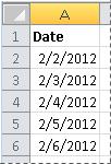
The text dates with two-digit years convert to standard dates with four-digit years.
Once you have converted the cells from text-formatted dates, you can change the way the dates appear in the cells by applying date formatting.
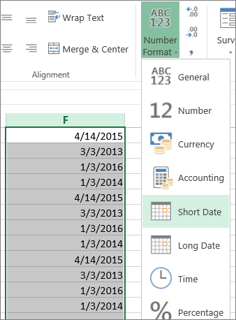
If your worksheet has dates that were perhaps imported or pasted that end up looking like a series of numbers like in the picture below, you probably would want to reformat them so they appear as either short or long dates. The date format will also be more useful if you want to filter, sort, or use it in date calculations.

-
Select the cell, cell range, or column that you want to reformat.
-
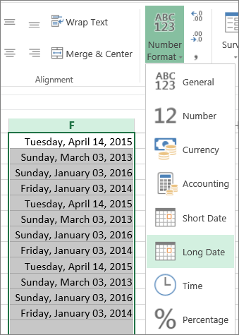
Click Number Format and pick the date format you want.
The Short Date format looks like this:
The Long Date includes more information like in this picture:
To convert a text date in a cell to a serial number, use the DATEVALUE function. Then copy the formula, select the cells that contain the text dates, and use Paste Special to apply a date format to them.
Follow these steps:
-
Select a blank cell and verify that its number format is General.
-
In the blank cell:
-
Enter =DATEVALUE(
-
Click the cell that contains the text-formatted date that you want to convert.
-
Enter )
-
Press ENTER, and the DATEVALUE function returns the serial number of the date that is represented by the text date.
What is an Excel serial number?
Excel stores dates as sequential serial numbers so that they can be used in calculations. By default, January 1, 1900, is serial number 1, and January 1, 2008, is serial number 39448 because it is 39,448 days after January 1, 1900.To copy the conversion formula into a range of contiguous cells, select the cell containing the formula that you entered, and then drag the fill handle
across a range of empty cells that matches in size the range of cells that contain text dates.
-
-
After you drag the fill handle, you should have a range of cells with serial numbers that corresponds to the range of cells that contain text dates.
-
Select the cell or range of cells that contains the serial numbers, and then on the Home tab, in the Clipboard group, click Copy.
Keyboard shortcut: You can also press CTRL+C.
-
Select the cell or range of cells that contains the text dates, and then on the Home tab, in the Clipboard group, click the arrow below Paste, and then click Paste Special.
-
In the Paste Special dialog box, under Paste, select Values, and then click OK.
-
On the Home tab, click the popup window launcher next to Number.
-
In the Category box, click Date, and then click the date format that you want in the Type list.
-
To delete the serial numbers after all of the dates are converted successfully, select the cells that contain them, and then press DELETE.
 across a range of empty cells that matches in size the range of cells that contain text dates.
Need more help?
You can always ask an expert in the Excel Tech Community or get support in the Answers community.
Need more help?
Want more options?
Explore subscription benefits, browse training courses, learn how to secure your device, and more.
Communities help you ask and answer questions, give feedback, and hear from experts with rich knowledge.
The date and time in Excel — there are numbers, formatted in a special way. The date is the integer part of the number, and the time (hours and minutes) is the fractional part.
By default, the number 1 corresponds to the date of 01. 01. 1900 — that is, each date — is the number of days passed from 01. 01. 1900. In this lesson, we will take a closer look at the dates, and in the next lessons – the time.
How in Excel to calculate the days between dates?
Since the date is a number, it means that you can conduct mathematical computing and settlement operations. To count the number of days between two Excel dates does not present any special problems. For a visual example, we first perform the addition, and then subtraction of dates. For this:
- On a blank sheet in the cell A1 you need to enter the current date by pressing CTRL +.
- In the cell A2 you need to enter an intermediate period in days, for example, 127.
- In the cell A3 you need to enter the formula: = A1 + A2.
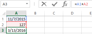
Note that the «Date» format was automatically assigned to the cell A3. It’s not difficult to guess, to calculate the difference in dates in Excel, you need to take away the highest date from the newest date. In the cell B1 you need to enter the formula: A3 — A1. Accordingly, we get the number of days between these two dates.
The calculating age by date of birth in Excel
Now we will learn how to calculate the age by date of birth:
- In the new sheet in the cells A1: A3, you need to enter the dates: 18. 04. 1985; 17. 08. 1977; 08. 12. 1992.
- In the cells B1 : B3, you need to put the current date.
- Now you need to use the function to convert the number of days to the number of years. To do this, you need to enter by manually the following value in the range C1:C3: = DATEDIF(A1; B1; «y»).
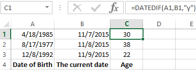
Thus, the application of the function allowed us to accurately calculate the age by date of birth in Excel.
Attention! To transform days into years, there is not enough of the formula: Moreover, even if we know that 1 day = 0.0027397260273973 of the year, the formula: =(B1-A1)*0.0027397260273973 will not give us the exact result either.
Days in the years the most accurately to convert the function: = DATEDIF(). You will not find it in the list of the function wizard (SHIFT+F3), but if you simply to enter it into the formula line, it will work.
The DATEDIF function supports to the several parameters:
| Option | Description |
| «d» | Count of full days; |
| «m» | Count of full months; |
| «y» | Count of full years; |
| «ym» | Count of full months without years; |
| «md» | Count of days without months and years; |
| «yd» | Count of days without years. |
Let’s illustrate the example of using several parameters:
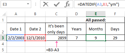
Attention! That the function: = DATEDIF() worked without errors, make sure that the start date was older than the end date.
The insertion of the date in the Excel cell
The purpose of this lesson is an example of mathematical operations with dates. Also, we’ll make sure that for Excel, the date data type is a number.
You need to fill in the table with dates, as shown in the picture:
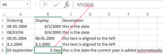
There are different ways of entering dates: in the column A there is input method, and in column B there is the display result.
Note that the default format cell is «General», the dates as well as the number are aligned on the right side, and the text on the left one. The value in the cell B4 is recognized by the program as text.
In the cell B7 Excel has assigned by itself to the current year (now is the 2015-th) by default. This is visible when displaying the contents of cells in the formula bar. Notice how the value was originally entered in A7.
The calculating of the Excel date
On the blank sheet in the cells A1 and C1 you need to enter 01. 01. 1900, and in the cells A2 and C2 is 01. 01. 1901. Now we change the format of the cells to «numeric» in the selected range C1:C2. To do this, you can press CTRL + SHIFT + 1.
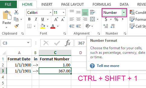
C1 contains now the number 1, and C2 — 367. That is, one leap year (366 days) now and one day passed.
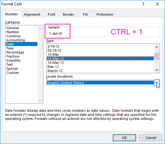
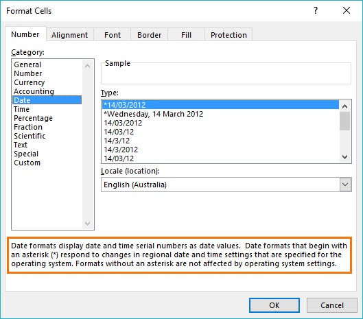
The way to display the date can be set using the «Format Cells» dialog box. To call it, press: CTRL + 1. On the «Number» tab, you need to select «Category:» — «Date». In the «Type:» section displays the most popular formats for displaying dates.
Download examples calculate date in Excel
Read also: The functions for working with dates in Excel
In the next lesson, we will work with the time and the periods of the day on ready-made examples.
The objective of this post is to teach you how Excel handles date and time and provide you with all the tools you will need.
It’s designed to be read in conjunction with the accompanying Excel file, which you can download below.
Download the Files
Enter your email address below to download the comprehensive Excel workbook and PDF.
By submitting your email address you agree that we can email you our Excel newsletter.
Regional Settings
When reading this post keep in mind that my regional settings format dates as dd/mm/yyyy and so the screenshots throughout this post are in this format. However, if you open the accompanying Excel file you may see some dates have switched to match your regional settings, which may be different to mine e.g. mm/dd/yyyy.
Dates and times with a format that begins with an asterisk (*) automatically update based on your PC’s regional settings. You can see an example in the Format Cells dialog box below:
Ok, let’s crack on.
Excel Date and Time 101
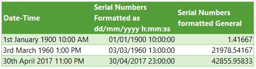
Excel stores dates and time as a number known as the date serial number, or date-time serial number.
When you look at a date in Excel it’s actually a regular number that has been formatted to look like a date. If you change the cell format to ‘General’ you’ll see the underlying date serial number.
The integer portion of the date serial number represents the day, and the decimal portion is the time. Dates start from 1st January 1900 i.e. 1/1/1900 has a date serial number of 1.
Caution! Excel dates after 28th February 1900 are actually one day out. Excel behaves as though the date 29th February 1900 existed, which it didn’t.
Microsoft intentionally included this bug in Excel so that it would remain compatible with the spreadsheet program that had the majority market share at the time; Lotus 1-2-3.
Lotus 1-2-3 was incorrectly programmed as though 1900 was a leap year. This isn’t a problem as long as all your dates are later than 1st March 1900.
Excel gives each date a numeric value starting at 1st January 1900. 1st January 1900 has a numeric value of 1, the 2nd January 1900 has a numeric value of 2 and so on. These are called ‘date serial numbers’, and they enable us to do math calculations and use dates in formulas.
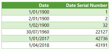
The Date Serial Number column displays the Date column values in their date serial number equivalent.
e.g. 1/1/2017 has a date serial number of 42736. i.e. 1st January 2017 is 42,736 days since 31st December 1899.
Tip: format the date serial number column as a Date and you’ll see they look the same as the Date column values.
Time
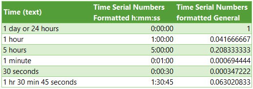
Times also use a serial number format and are represented as decimal fractions.
Hours: since 24 hours = 1 day, we can infer that 24 hours has a time serial number of 1, which can be formatted as time to display 24:00 or 12:00 AM or 0:00. Whereas 12 hours or the time 12:00 has a value of 0.50 because it is half of 24 hours or half of a day, and 1 hour is 0.41666′ because it’s 1/24 of a day.
Minutes: since 1 hour is 1/24 of a day, and 1 minute is 1/60 of an hour, we can also say that 1 minute is 1/1440 of a day, or its time serial number is 0.00069444′
Seconds: since a second is 1/60 of a minute, which is 1/60 of an hour, which is 1/24 of a day. We can also say one second is 1/86400 of a day or in time serial number form it’s 0.0000115740740740741…
Date & Time Together
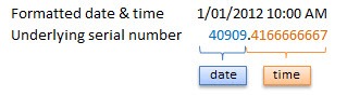
Now that we know how dates and times are stored we can put them together — ddddd.tttttt
For example, the date and time of 1st January 2012 10:00:00 AM has a date-time serial value of 40909.4166666667
40909 being the serial value representing the date 1st January 2012, and .4166666667 being the decimal value for the time 10:00 AM and 00 seconds.
More examples below.
Entering Dates & Times in Excel
Entering Dates
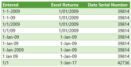
You can type in various configurations of a date and Excel will automatically recognise it as a date and upon pressing ENTER it will convert it to a date serial number and apply a date format on the cell.
For example, try typing (or even copy and paste) the following dates into an empty cell:
| 1-1-2009 |
| 1-1-09 |
| 1/1/2009 |
| 1/1/09 |
| 1-Jan-09 |
| 1-Jan 09 |
| 1-Jan-2009 |
| 1 Jan 09 |
| 1/1 |
You can see in the table above that entering numbers that look like dates and are separated by a forward slash or hyphen will be recognised as a date. Even typing in a date with the month name gets converted to a date.
However, dates separated with a period like this 1.1.2009, or with spaces between numbers like this 01 01 2009, will end up as text, not a date. Gotta have some limits!
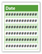
Tip: Dates that display ##### in a cell usually indicate that the column is simply not wide enough to display it.
However, if you make the cell really wide and it still displays ##### then this indicates that the date is a negative value and Excel can’t display negative dates.
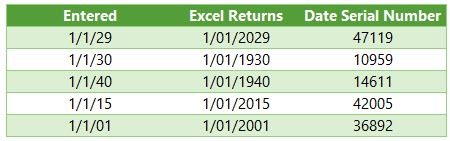
Entering Dates with Two Digit Years
When you enter a date with two digits for the year e.g. 1/1/09, Excel has to decide if you mean 2009 or 1909.
It goes by the rule that dates with years 29 or before, are treated as 20xx and dates with the year 30 or older are treated as 19xx. See examples below.
Tip: You can enter the day and month portions of a date and Excel will insert the year based on your computer’s clock. Nice to know for data entry.
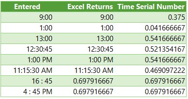
Entering Time
When you enter time you must follow a strict format of at least h:mm. i.e. the hour and minutes are separated by a colon with no spaces either side. Entering the h:mm components will result in a time formatted in military time e.g. 2:00 PM is 14:00 in military time.
If you enter a time that includes a seconds component e.g. 3:15:40, Excel will automatically format the cell in h:mm:ss.
If you want the time to be formatted with AM/PM you can simply enter a space after the time and then type AM or PM, or apply the number format to the cell later. Here are some examples:
Entering Dates & Time Together
Now that we know how to enter dates and time separately we can put them together to enter a date and time in the same cell.
You can even enter time then date and Excel will fix the order for you.
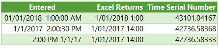
You’ll find that even if you enter AM/PM, that Excel will convert it to military time by default. You can override this with a custom number format. More on that later.
Simple Date & Time Math
Now that we understand that Excel stores dates and time as serial numbers, you’ll see how logical it is to perform math operations on these values. We’ll look at some simple examples here and tackle the more complex scenarios later when we look at Date and Time Functions.
Adding/Subtracting Days from Dates
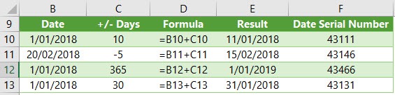
Tip: you can also add/subtract the days directly in the formula e.g. =B10+10 or =B11-5 Although, it’s better to place the values you’re adjusting by in their own cell or a named range.
Subtracting Dates from one another
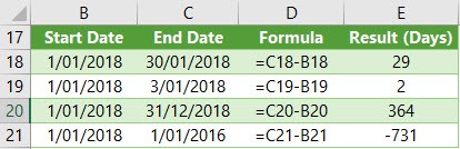
Tip: format the cell to General or Number to see the number of days between two dates.
Note: the ‘result’ is exclusive of the start day i.e. it assumes the start day is at the end of that day.
Adding Times to one another
The time being added is input as a time serial number. Notice there are no negative times in the table below. Remember we can’t display negative times. Instead we need to use the math operator to tell Excel to subtract time. See examples below.
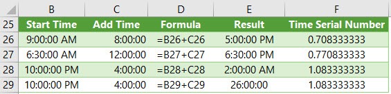
Note: Times that roll over to the next day result in a time-date serial number >= 1. Cell E28 actually contains a time-serial number of 1.08333′, but since the cell is formatted to display time formatted as h:mm:ss, only the time portion is visible.
If you want to show the cumulative time (like cell E29) then you need to surround the ‘h’ part of the time format in square brackets like so: [h]:mm:ss
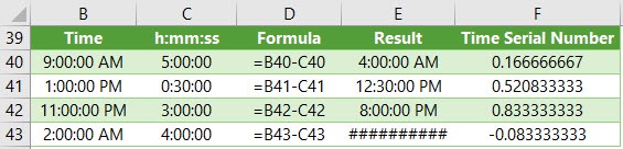
Subtracting Time from Times
Notice the last result in the table below shows ######, this is because it results in a negative time and Excel can’t display that, but notice it can return a negative time serial number. More on how to solve this later.
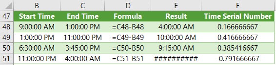
Subtracting Times from one another
Again, here the last result shows ###### because it results in a negative time.
Excel Date and Time Shortcuts
‘Good to Know’ Stuff about Excel Date and Time
— Dates prior to 1st January 1900 are not recognised in Excel.
— A negative date will display in the cell as #######
— Times stored without a date effectively inherit the date 0 Jan 1900 i.e. the month is Jan and the year 1900 and the day is zero. Remember, there are no dates prior to 1/1/1900 from Excel’s perspective. This means that times stored without a date e.g. 0.50 for 12:00 PM is the equivalent of 0 Jan 1900 12:00 PM.
This is important because if you try to take 14 hours from 12 hours (without a date) you’ll get the dreaded ###### display in the cell, because negative dates and times cannot be displayed. We’ll cover workarounds for this later, but for now keep in mind that math on dates and time that result in negative date-time serial numbers cannot be formatted as a date.
Date Modes
— Excel actually has two date modes. The other mode is called 1904 Date System and is used for compatibility with Excel 2008 for Mac and earlier Mac versions. You can change the date system in the Advanced Options.
In the 1904 date system dates are calculated using 1st January 1904 as the starting point. The difference between the two date systems is 1,462 days. This means that the serial number of a date in the 1900 date system is always 1,462 days greater than the serial number of the same date in the 1904 date system. 1,462 days is equal to four years and one day (including one leap day).
Caution; the date setting you choose applies to all dates within the workbook. You can’t mix and match modes and you shouldn’t reference workbooks that use a different date system in formulas.
Bottom line; don’t use the 1904 date system unless absolutely necessary! Click here for more on date systems in Excel.
— Excel applies date number formats based on your system region settings. For example, my system is set to display dates in dd/mm/yyyy format, but if you’re in the U.S. your system is likely to format them as mm/dd/yyyy. Excel will automatically convert the format of date serial numbers to suit your system settings as long as it’s one of the default date formats and not a custom number format.
More Excel Date and Time Tips
This post is just the beginning, the next steps in mastering Excel Date and Time are below:
- Every Excel Date and Time Function explained
- Formatting Date and Time in Excel
- Common Date and Time Calculations
Tip: Avoid waiting, download the workbook and get the above topics now.
Enter your email address below to download the comprehensive Excel workbook and PDF.
By submitting your email address you agree that we can email you our Excel newsletter.
Explanation
When date information from other systems is pasted or imported to Excel, it may not be recognized as a proper date or time. Instead, Excel may interpret this information as a text or string value only. In this example, the goal is to extract valid date and time information from a text string and convert that information into a datetime. It is important to understand that Excel dates and Excel times are numbers so at a high level, the main task is to convert a text value to the appropriate numeric value.
Date
To get the date, we extract the first 10 characters of the value with the LEFT function:
LEFT(B5,10) // returns "2015-03-01"
The result is text, so to get Excel to interpret as a date, we wrap LEFT in DATEVALUE, which converts the text into a proper Excel date.
Time
To get the time, we extract 8 characters from the middle of the text with the MID function:
MID(B5,12,8) // returns "12:28:45"
Again, the result is text. To get Excel to interpret this value as time, we wrap MID in TIMEVALUE, which converts the text into a proper Excel time.
Datetime
To get a final datetime, we just add the date value to the time value. The formula in E5 is:
=C5+D5
Once you have a valid datetime, use custom number formatting to display the value as desired.
All in one formula
Although this example extracts the date and time separately for clarity, you can combine formulas if you like. The following formula extracts the date and time, and adds them together in one step:
=LEFT(date,10)+MID(date,12,8)
Note that DATEVALUE and TIMEVALUE aren’t necessary in this case because the math operation (+) causes Excel to automatically coerce the text values to numbers.
Return to Excel Formulas List
Download Example Workbook
Download the example workbook
This tutorial will demonstrate how to convert a date to a serial number corresponding to that date (or vis-a-versa) in Excel and Google Sheets
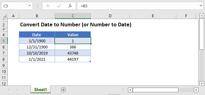
Date to Number
To convert a date to a serial number, all you need to do is change the formatting to General:
However, this won’t work if the date is stored as text.
Date Stored as Text to Number
If the date is stored as text, you can use DATEVALUE convert it to an Excel date:
=DATEVALUE(B3)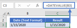
Then you can change the formatting to general to see the serial number.
Number to Date
To convert a serial number to a date, all you need to do is the change the formatting from General (or Number) to a date format (ex. Short Date):
Convert Date to Number in Google Sheets
All of the above examples work exactly the same in Google Sheets as in Excel.
All Excel’s Date and
Time Functions Explained!
Written by co-founder Kasper Langmann, Microsoft Office Specialist.
This is the complete guide to date and time in Excel.
It’s a whopping +5500 words (!), so be sure to bookmark it.
The first part of the guide shows you exactly how to deal with dates in Excel.
I will show you how to perform calculations involving dates. We’re also going to look at some of Excel’s (awesome) built-in functions. These allow you to extract just what you need from data that includes dates.
In the second part of the guide, I’ll show you how to work with time data in a spreadsheet.
This is going to be a lot of fun. Grab a cup of coffee, and let’s start rolling!
 Kasper Langmann, Co-founder of Spreadsheeto
-
7: Date formatting
- What is date formatting?
- How to use other date formats (from the ‘Format Cells’ dialog box)
- How to use custom date format
- Turn text into dates with the DATEVALUE function
- How to auto populate date in Excel when a cell is updated
- How to insert a date picker in Excel
Get your FREE exercise file
Before you start:
Throughout this guide, you need a data set to practice.
I’ve included one for you (for free).
Download it right below!
Introduction to
calculations with dates
When analyzing and manipulating date information in Excel, you have several formatting options.
In other words, you can display your data in many ways.
Most of the time, Excel will know that you are entering a date when you key in the data like the following:
- 1/1/2017
- January 1, 2017
- 1-Jan
The clearest sign that Excel has stored your data in a cell as a date is that it should be right-aligned in the cell.
Kasper Langmann, Co-founder of SpreadsheetoBelow are a few examples of the various formats that Excel displays dates in.
But the key is that they are all aligned to the right of the cell.

Contrast column A with column B (where the cells are formatted as text). They show the same information.
But, the alignment to the left side of the cell indicates that they are not formatted as a date. As you will soon see, this presents problems when performing calculations with dates.
Kasper Langmann, Co-founder of SpreadsheetoOne important note about how Excel stores dates:
To use dates in calculations, Microsoft Excel stores dates as serial numbers.
These are the sequential number of the day in relation to the starting date of January 1, 1900.

So, think of January 1, 1900, as serial number 1.
January 1, 2016, would be serial number 42370 as it’s 42,370 days after January 1, 1900.
For this reason, dates need to be in a date format rather than text format. If stored in text format, their serial number will not be stored in Excel. This is a no-go as you need these serial numbers when you want to perform calculations involving dates.
Kasper Langmann, Co-founder of SpreadsheetoHow to add time to dates in Excel
Now you know the fundamentals of date formatting versus date data formatted as text. Let’s look at some calculations you can do with dates.
First, why don’t we look at how to add days to a date?
Kasper Langmann, Co-founder of SpreadsheetoHow to add days to a date
Adding days to a date is very simple, straightforward, and intuitive.
All you need to do is add the number of days as a single number to the date or cell reference containing the date.
The following figure illustrates just how simple it is to add 1 day or 90 days to a date.

How to add months to a date
If you need to add a month or several months to your date, the process is a bit more complicated.
For this calculation, you will need to call upon the built-in Excel function, EDATE. The syntax for EDATE is so simple, that you will pick it up in no time at all.
Kasper Langmann, Co-founder of SpreadsheetoHere’s its syntax:
=EDATE(start_date, months)
The function requires 2 arguments: ‘start_date’ and ‘months’.
The first, ‘start_date’, is simply the date we are adding months to.
The second, ‘months’, is the number of months we would like to add to the date.
Look at the figure below to see just how easy it is to calculate a new date by adding 6 months and 9 months to the start date.

How to add years to a date
So, what about calculating the addition of years to your original date?
For this, you need to use a few more functions. But, as noted before, this is super intuitive so don’t let the length of these formulas fool you.
Kasper Langmann, Co-founder of SpreadsheetoThe first function we need to focus on is DATE.
The syntax for DATE is also incredibly simple and intuitive:
=DATE(year, month, day)
But, for our purposes, we can use the YEAR, MONTH, and DAY functions along with DATE.
These functions extract the correct data from our original date. This ensures appropriate use of our final DATE formula.
For example, applying MONTH to a cell reference of our original date will extract the month data. The same is true for YEAR and DAY.
So, we will place these functions in the appropriate argument within the DATE function. And if we want to add 1 year to the date, we simply place a ‘+1’ after the YEAR function in the ‘year’ argument of the DATE function.
Kasper Langmann, Co-founder of SpreadsheetoThat was a lot, so let’s look at the following figure to see it in action.

Notice row 18 and column C of the worksheet.
The ‘year’ argument of the ‘DATE’ function is substituted by the function ‘YEAR(A18)+1’.
This tells the DATE function that we want the year only from the date data in A18 (or 2017) – and that we want to add ‘1’ to it (or 2018).
How to subtract dates
Adding time to a date is super useful.
But what if you had a report where you needed to calculate the difference between dates?
This is where we turn our attention to subtracting dates…
Kasper Langmann, Co-founder of SpreadsheetoFind the difference between two dates
To find the difference between two dates, we want to turn our attention to the DATEDIF function.
The most important thing you need to know about DATEDIF is that it is a hidden function. What that means is that it will not be found in the visible list of Excel functions on the formula tab.
Kasper Langmann, Co-founder of SpreadsheetoThis requires you to type the formula in its entirety.
There will be no tooltip hint as you begin to type the function.
Let’s look at the syntax:
=DATEDIF(start_date, end_date, unit)
There are three arguments for the DATEDIF function:
- start_date: This is the initial date of the period among the two you are calculating the difference between.
- end_date: This is the latest date of the two.
- unit: This is the unit in which you want the function to return the difference by. More on units right below…
The ‘unit’ argument gives you a choice of several formats to return your results from DATEDIF.
- y – The number of complete years between dates.
- m – The number of complete months between dates.
- d – The number of days between dates.
- md – The number of days ignoring months and years.
- yd – The number of days ignoring years.
- ym – The number of months ignoring days and years.
So, let’s look at a few examples using DATEDIF in various forms.
Kasper Langmann, Co-founder of Spreadsheeto
In our example, you can use literal dates if they are enclosed in double quotes.
You can also use the serial number format as shown in rows 4 and 5.
Now note the difference in the returned value between row 2 and 3. The ‘start_date’ and the ‘end_date’ are unchanged. But, our results are different. The first formula returns the total number of days between the dates.
Kasper Langmann, Co-founder of SpreadsheetoBut in the second example, we use ‘md’ for the unit argument. ‘md’ is the difference between the dates in days – ignoring the months and years. That is 15 minus 1, or 14 days.
You can also calculate the difference between two dates in cells.
To do this, place the cell reference of your dates in the ‘start_date’ and ‘end_date’ arguments.

One (last) important thing to note about using DATEDIF:
The ‘end_date’ argument must always be later than the ‘start_date’ or you will get the ‘#NUM!’ error.
Use today’s date in Excel
Now let’s turn our attention to some tricks and shortcuts involving the current date.
Often, you need to work with the current (today’s) date.
There are some nifty tricks that allow you to do this without typing in the entire date manually.
Let’s look at them!
Use date that updates itself with the TODAY function
One of the simplest ways to input today’s date into a cell is to use the TODAY function.
Do this by typing ‘=TODAY()’ into a cell.
This places the current date into the cell dynamically. So, that cell would have tomorrow’s date in it if you reopen the file tomorrow.
You can also nest the TODAY function within the DAY or MONTH function. This return only the current day or current month in a cell. Refer to the following figure to see the TODAY function in action.
Kasper Langmann, Co-founder of Spreadsheeto
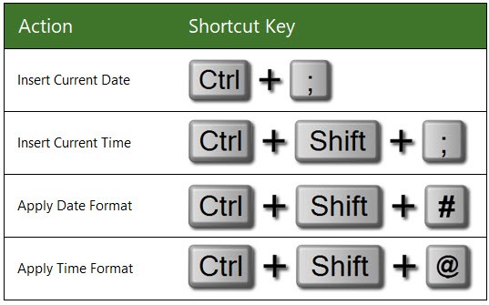
Insert static current date in Excel using shortcuts
You can also insert the current date using keyboard shortcuts.
For the current date, press the following key combination:
Ctrl + ;
To insert both the date and the time, press the previous keyboard shortcut. Then press the following combination:
Ctrl + Shift + ;
These shortcuts enter static dates and times. This opposed to the dynamic date that the TODAY function returns.
Subtract a date from the current date
You can use the current date in a calculation like subtracting.
You replace the ‘start_date’ argument in the DATEDIF formula.

Above image shows how to substitute the TODAY function for a literal date value or cell reference for the ‘start_date’ OR the ‘end_date’.
Remember the rule that the ‘end_date’ must be later than the ‘start_date’ still applies.
Using the TODAY function in a calculation is useful when you need to track a time period dynamically. Say you need to calculate some sort of countdown to a deadline. Using the TODAY function in your calculation is the perfect way to do this.
Kasper Langmann, Co-founder of SpreadsheetoYou can also use the keyboard shortcut to insert the current date if you need to insert the static date. This is a quicker and more efficient way to insert today’s date.
Retrieving numbers from dates
with Date functions
There are often situations where you need to retrieve numbers from dates.
But, you might not have the need for an entire date.
Let’s say you have a report. Here you want to separate the different elements of the date for filtering by a single element of the date – like the month or year.
Here’s how to go about doing that 🙂
Use the DAY function to find the day of a date
To isolate only the day of the full date, we use the DAY function.
There is a single argument for the DAY function:
=DAY(serial_number)
You probably know by now that ‘serial_number’ is the date.
This argument can be the actual serial number form of the date or the literal date in double quotes. It can also be a cell reference like in the following example.

Look at above picture again. Notice that regardless of the format of your original date, the DAY function returns the value ‘14’.
Use the MONTH function to find the month of a date
If you need to isolate the number value for the month of your original date, you can use the MONTH function.
It works the same way the DAY function works:
=MONTH(serial_num)

Use the YEAR function to find the year of a date
Now we move onto the function that retrieves the number value for the year part of the date.
The syntax for the ‘YEAR’ function is like the DAY and MONTH functions syntactically.
=YEAR(serial_num)
You already know how to retrieve the day and month number values. It’s the exact same concept when using the ‘YEAR’ function.

Use the WEEKDAY function to find the day of the week
You can also retrieve the number value for the day of the week from a date.
The WEEKDAY function returns the number that corresponds to the day of the week. For instance, 1 for Sunday, 2 for Monday, 3 for Tuesday, and so on.
Kasper Langmann, Co-founder of SpreadsheetoHere’s its syntax:
=WEEKDAY(serial_num, [return_type])
The syntax for WEEKDAY requires the ‘serial_number’ argument.
It also allows for an optional argument: ‘return_type’.
This allows you to choose a different start and end date for your week.
That means that the returned value will align with that chosen sequence.
Below you can see the list of different ‘return_type’ values that Excel allows.

In the following examples, note the value differences returned by the formula based on the ‘return_type’ argument.

The different selections for the ‘return_type’ in the formulas return very different weekday values.
These depend on the first day of the week that corresponds to those ‘return_type’ values.
Use the WEEKNUM function
to find out the week number
Another interesting built-in function is the WEEKNUM function.
WEEKNUM retrieves the number value for the week of the year that the original date falls within (1 – 52).
So, if the original date is between January 1 and January 7, the WEEKNUM value would be ‘1’.
If the date is between December 25 and December 31, WEEKNUM would return the value ‘52’.
=WEEKNUM(serial_number, [return_type])
The ‘return_type’ argument corresponds to different days you can choose as the start day. This changes the week number based on what day of the week that the ‘return_type’ sets as the first day of the year.
Kasper Langmann, Co-founder of Spreadsheeto
Our date falls on a Monday.
The result of the WEEKNUM formula will be different if the ‘return_type’ argument is ‘1’ (Sunday) versus ‘12’ (Tuesday).
This can be useful since the calendar year begins on different days of the week. This comes in handy if want to calculate the week number based on the first full week of the year.
Kasper Langmann, Co-founder of Spreadsheeto
This can be a very useful function.
Consider a situation in which you needed a weekly countdown. Simply calculate the difference between dates using the WEEKNUM function.
Use the WORKDAY function to calculate the number of working days between two dates
Another useful function is the WORKDAY function.
This function returns a day that is some number of workdays into the future or before some date. A “workday” is days excluding weekends and any holidays that are specified.
The function requires two arguments and has an optional third.
=WORKDAY(start_date, days, [holidays])
- start_date – this required argument is the date from when you want to count the number of workdays
- days – this required argument is the number of days from the start date you want a count of. Using a negative number will give you the date that many workdays before your start date.
- holidays – this argument is optional. This allows you to add holiday dates in the formula for the WORKDAY function to skip along with weekends.
This is a bit more complex than the functions we have been discussing. Let’s look at a few examples to help the concept of the WORKDAY function sink in.
Kasper Langmann, Co-founder of Spreadsheeto
First, note that we have listed 3 holiday dates in cells A8, A9, and A10. We will be using these in our examples for the ‘holiday’ argument to exclude along with weekends.
On row 2, we want to know the date that is 90 workdays from Monday, November 14, 2016.
Excluding the weekends and holidays (A8:A10), this will be Tuesday, March 21, 2017 according to the WORKDAY function.
On row 3, we can instantly see the effect of weekends and holidays on the outcome of our formula. We want the date that is 2 workdays from Wednesday, November 23, 2017.
Because of the holiday on Thursday, November 24 – and the weekend days Saturday and Sunday – the result is Monday, November 28, 2016.
This example illustrates how powerful the WORKDAY function can be. It calculates something very simple. Yet, if done manually, this is a very cumbersome process.
Kasper Langmann, Co-founder of SpreadsheetoThe third example in the figure illustrates how to use WORKDAY to find a date before the start date.
We want to know the date that is 20 workdays before Monday, January 17, 2017.
So, our DAY argument needs to be a negative value (-20).
Again, note the result considers weekend days as well as a couple of holidays.
How to auto fill dates
In this section, we are going to cover how to work with sequences of dates. This time by using the autofill capability of Microsoft Excel.
You can use Autofill in 2 ways.
The first is to double-click the fill handle. The fill handle is a small square that appears in the lower right corner of a highlighted cell.
The second option is to simply drag the handle to the desired cell. Note the fill handle for the highlighted cell in the following figure.

The fill handle also offers some more options.
Try to right-click and drag outside the selection a bit.

We will focus on the selections that fill elements of the date like days, weekdays, months, and years.
Insert dates that increase by one day
To insert dates that increase by one day in a column, you can simply grab the fill handle.
Then drag it down as many rows as you need dates for.
One thing to take note of is that as you do this, Excel shows the incremented date as you drag the range.
So, you can see just what date you are at as you expand the range.

Once you release the fill handle, your range is now filled with dates.
These dates increment in one-day intervals.

Insert dates that increase by weekdays
But what if you wanted to increment a wide range of dates by weekdays only?
This is easily done by selecting ‘Fill Weekdays’ from the ‘Autofill Options’ that appears once you fill the dates down.

Once you select ‘Fill Weekdays’, Excel automatically excludes any weekend dates from the range.

Insert dates that increase by months and years
You can also use the ‘Autofill Options’ to increase months and years.
Select the fill option you need once you fill the dates down to the last cell of your range.
Insert dates that increase by several days
I’m sure you can think of other custom intervals (dates) you might like to fill down your column (or row, for that matter).
Microsoft Excel allows for a little of that also.
So, what if you wanted to increment every other day? Or what about every 3 months?
These other intervals are available using auto fill. Drag down the dates by using the fill handle. Then right click and hold on the fill handle while moving the cursor slightly outside the range. Now release until you see the options menu.
Kasper Langmann, Co-founder of Spreadsheeto
Click on ‘Series…’. The Series dialog box will now open.
This gives you several options for customizing the intervals of your dates.

For our example of every other day, you can select a Step value of ‘2’.
Leave everything else as it is.

Date formatting:
Make a date easy to interpret
In the beginning of this tutorial, I told you about the differences between text format and date format.
Now, we’re going to take a deeper dive into formatting of dates. We can represent date data in different date formats. These are easily adjusted according to our preferences and needs.
Kasper Langmann, Co-founder of SpreadsheetoAlso, remember our point earlier, that Excel stores date data as serial number.
So, no matter what date format you choose, Excel still recognizes it as a serial number.
What is date formatting?
Date formatting offers you choices on how you want to represent the date data in your worksheets.
Let’s look at our original example at the beginning of this tutorial.
We can see in the Number group of the Home tab that our data cells are all formatted as Date.

If you take the same data and place it into another column, something interesting happens.
In the cells that are formatted as ‘General’, you’d see the dates serial numbers.

If you run into this in your own spreadsheets, you must know how to fix this…
It’s quite simple, you just need to know how to reformat those cells into the Date format that you need.
For this example, let’s reformat to ‘Short date’.
Highlight the cell containing the serial number. Click on the drop-down arrow to see all the available formats in the Number group of the Home tab.

Select ‘Short Date’ from the dropdown and now the serial number will be converted from ‘General’ format to a date format that you recognize.

How to use other date formats
from the ‘Format Cells’ dialog box
You’ve now seen how to change date data formatted as ‘General’ to the ‘Short Date’ format.
Now we look at some other date formats that Excel also offers…
You already know how to change to a date format from the ribbon but you can also use the ‘Format Cells’ dialog box.
The first step is to find the cell that contains the serial number you want to reformat.
Then, right-click on the cell.
Select ‘Format Cells’ from the menu that appears.

From the Format Cells dialog box, select ‘Date’ in the Category box.
This reveals the different standard date format types available in Excel.
You find these formats in the Type box on the right side of the Format Cells dialog box. As you change Type selections, you can view a sample of the actual value in the cell you have selected in the Sample box.
Kasper Langmann, Co-founder of Spreadsheeto
Decide on the ‘Type’ you want.
Then click ‘OK’ and the serial number now changes to the date format type you selected.

How to use custom date format
Even with all the date types Excel offers, you can still format your date data with your own custom format.
It is pretty simple to do…
Follow the same steps as we did with the previous example.
But, instead of choosing ‘Date’ in the Category box in the Format Cells dialog box, select ‘Custom’.

Take a second look at the picture above.
Here the Format Cells dialog box shows the current format of the cell in the Type and Sample boxes.
Now you can select from the various default types available. You can also edit those types in the Type box or type in one that is completely custom.
Kasper Langmann, Co-founder of SpreadsheetoLet’s clear out the Type box…

And then type “mm-dd-yyyy” into that box:

Again, note that as we do this, the Sample box shows us our exact data as it will look under our new custom format. Click ‘OK’ and you are done creating your own custom date format.
Kasper Langmann, Co-founder of SpreadsheetoTurn text into dates with the DATEVALUE function
Another method for converting dates in text format is to use a function called DATEVALUE.
This function converts text string dates to their appropriate serial numbers.
These serial numbers are, as you know by now, the way Excel recognizes dates. You can format this output according to the methods I’ve shown you in the prior sections.
Kasper Langmann, Co-founder of SpreadsheetoThe DATEVALUE syntax is simple:
=DATEVALUE(date_text)
So, let’s look at a few examples of cells containing dates that are in text string form.
Let’s use the DATEVALUE function in the column next to these cells.
Here it’s easy to see if the cells return the serial numbers we expect.

If your text date is before the year 1900, the DATEVALUE function will return the ‘#VALUE!’ error.
That’s because Excel recognizes dates as serial numbers beginning at January 1, 1900.
If your text date doesn’t contain a year, the DATEVALUE function defaults to the current year from your system clock.
How to auto populate date when a cell is updated
What if you wanted to make sure each time a cell’s data got updated, you knew when it was updated?
You could input the date and time manually in the cell next to it.
But what if you wanted to automate that process?
That way you’ll never forget to do it. Also, you would mitigate the chances for a data entry error.
There are several ways to approach this. One of the best ways is to use VBA to create a worksheet change event. It is a macro that automatically runs when a cell’s value changes.
Kasper Langmann, Co-founder of SpreadsheetoA quick recommendation:
Excelribbon.tips.net has written an awesome guide that demonstrates a worksheet change event. Make sure to check it out!
How to insert a date picker in Excel
Another cool thing you can do in Excel with dates is to create a date picker. This allows users to choose a date from a preset dropdown calendar. That way they don’t have to input the date by hand.
This is actually a pretty complex proposition in Excel. But if you want to see a date picker and a bit about how one can be created using VBA. Contextures has an amazing guide to do it right here.
Calculations with Time
Maybe you need to quantify elapsed time for tasks or projects?
Or perhaps you need to insert a time rather than a date in your data?
There are many parallels between the techniques of working with dates and time.
How to add time in Excel
Let’s look at a scenario where you have documented the total time it took for two different tasks in Excel.
Now you want to add those together to get your total time worked.
This is as simple as clicking on the cell below the task times and pressing Alt + = to autosum the times.

Now let’s look at a scenario where you have the times worked for a full workweek that you need to add together for a total.
If we autosum once again, we immediately notice a problem.

We know by simple inspection that these workday time values add up to more than 12 hours and 52 minutes.
Excel can display times in a variety of ways. For instance, hours and minutes, 12-hour format, and 24-hour format, and several others.
Kasper Langmann, Co-founder of SpreadsheetoWhat we need to do in our current situation is to right click on the cell where our auto sum formula is.
Then select Format Cells like we did with dates.

Then select ‘Custom’ from the Category box and clear the Type box.
Then in the Type box, type ”[h]:mm”.
Click ‘OK’ and you should have the correct total of hours for the week now.

How to find the difference between two times
Finding the difference between times is not quite as simple as adding times together.
Let’s look at a situation where we have a start time and an end time and we want to calculate the total elapsed time.

In cell B4, type the formula ‘=(B3-B2)*24’.
This subtracts the end time from the start time and then multiplies both by 24.
The multiplication by 24 is required since Excel recognizes times as a fraction of a full 24-hour day.

Our result is a numerical value and we choose to set it to two decimal places to show fractions of a full hour.

If you want to see the elapsed time in the actual hours and minutes, here’s what to do.
Remove the ‘*24’ and format using the custom format we created in the previous example adding times ([h]:mm).
Find current time in Excel
The NOW function allows you to insert the current time based on your computer’s system clock.
NOW returns the current date and time whereas TODAY returns the current date only.
But we can use NOW and format our cell so that it only shows the time but not the date.

Insert static current time with shortcuts
You’ve already seen the keyboard shortcut for entering in the static current date as well as entering the static current time.
Since we are discussing time data, I’ll show you how to use a keyboard shortcut to enter the static current time.
All you must do is press the following keyboard combination:
Ctrl + Shift + ;
Again, this contrasts with using the NOW function because it is static rather than dynamic.
This keyboard shortcut inserts the exact time you pressed the keyboard shortcut. It will remain that time unless you manually change it.
Retrieve seconds, minutes and hours
Let’s look at retrieving parts of time data.
This is very much the same as when you retrieved the month, day, and year, from dates. We are going to retrieve the seconds, minutes, and hours with some built-in functions available in Excel.
If you want to retrieve the seconds from a time value in Excel, you use the built-in SECOND function.
There is a single required argument for this function: ‘serial_number’.
=SECOND(serial_number)
Let’s look at a few simple examples to see this function in action:

For times that don’t display the seconds, the SECOND function still retrieves the seconds from the serial number of the date.
If you need to retrieve the minutes from your time data, you want to use the MINUTE function. Like with SECOND function (and others), there is only the required ‘serial_number’ argument.
=MINUTE(serial_num)
Now we will take the same time data we used for the SECOND function and use the MINUTE function.

The last thing we will look at is the HOUR function. Nothing new on the syntax.
=HOUR(serial_number)
One thing to note about the HOUR function is that it returns a value for the hour based on 24 hours.
So, if you want your HOUR function to return the hour in an AM/PM fashion, subtract 12 from your function if it is a time later than 12 PM.

Formatting time: What is it?
Just like with dates, there are several different format types for time data.
In fact, our examples so far have demonstrated a few of these different formats.
You may want to display times in 12-hour format or 24 hours. You might want your 12-hour format times to show AM and PM, or you may not.
Kasper Langmann, Co-founder of Spreadsheeto
You find the default time format types by right-clicking a cell.
Then select Format Cells.
Note in the figure above how many variations you can choose from. You can always create your own custom format by selecting ‘Custom’ from the Category list.
How to use and change time formatting
Now we have reviewed how you select different time formats.
Let’s look at a few examples of the different types.
We will look at 3 different selections from those available in the types for time formats.
The first thing we need to do to change format is to right click on the range of dates we want to reformat. Then select Format Cells.

Once the Format Cells dialog opens, select ‘Time’ from the Category box. Then in the Type box select ‘*1:30:55 PM’.

The asterisk in ‘*1:30:55 PM’ indicates that this format changes to the Region settings on your computer.
Any changes to the Windows time format settings will reflect in Excel. But only for the times formatted with a format preceded by an asterisk.
So, we format column B times as ‘*1:30:55 PM’ and then two other formats in columns C and D for the sake of contrast. Look at the different format variations in the following figure.
Kasper Langmann, Co-founder of Spreadsheeto
Turn text into time with the TIMEVALUE function
The DATEVALUE function converts dates in text string form to date formatting.
Like DATEVALUE, the TIMEVALUE function converts text string time data to actual time format.
See the syntax here:
=TIMEVALUE(text_time)
The ‘text_time’ argument is required. It is simply the text string date that you need to convert to time format.
One thing to recall is that Excel recognizes time as a fraction of 24 hours. For instance, 12 pm would be interpreted by Excel as .5 since it is the halfway point of the 24-hour day.
Kasper Langmann, Co-founder of SpreadsheetoSo, when you use the TIMEVALUE function, you won’t get a time.
Rather, it returns a decimal number value that is a fraction of the entire day.

If you multiply the TIMEVALUE result by 24, you get a more accurate interpretation of the time (albeit still in decimal format).

But if you reformat the TIMEVALUE result to a time format, you are good to go.
You will have changed a text string time to a true time format that Excel will now recognize as time instead of text.
Wrapping up
There it is, the most comprehensive guide to date and time in Excel.
It’s taken us tons of hours and resources to publish. Feel free to share it along with anyone who needs to brush up their dates and times 😊
If you enjoyed this tutorial, I’m sure you’ll love this…
Kasper Langmann2020-05-11T13:30:38+00:00
Page load link
The DATEDIF function is categorized as a DATE/TIME function in Excel. The function name almost gives away its purpose. It calculates the difference (DIF) between two given dates (DATE). This function is particularly useful for financial analysts. For instance, when they need to calculate the holding period in terms of days, months, or years.
DATEDIF is an undocumented function, this means you would not find this function in the formula tab. In addition to this, Excel will also not help you with IntelliSense (the suggestions Excel provides while you type function syntax) while writing the DATEDIF function, but it works well when configured correctly.

Note: Please note that DATEDIF Function in Excel is totally different from the DATEDIFF (notice the extra ‘F’) function in VBA.
Syntax
Learning the syntax of the DATEDIF function is crucial since Excel won’t help you with IntelliSense. The syntax is as follows:
=DATEDIF(start_date, end_date, unit)
Arguments:
‘start_date‘ – This is a required argument where you will need to insert the starting date.
‘end_date‘ – This is a required argument where you will need to insert the ending date.
‘unit‘ – This argument is supplied as a text string and represents the units in which we want the formula to compute the difference. You may use the table given below for appropriate codes required for the desired results.
Codes for Unit Argument
| UNIT | DESCRIPTION |
|---|---|
| «Y» | Returns difference as complete years. |
| «M» | Returns the difference as complete months. |
| «D» | Returns the difference in days. |
| «MD» | Returns the difference in days, ignoring months and years. |
| «YM» | Returns the difference in months, ignoring years. |
| «YD» | Returns the difference in days, ignoring years. |
Important Characteristics of the DATEDIF function
- The DATEDIF function is an undocumented compatibility function inherited from Lotus 1-2-3. When you start typing the DATEDIF function, Excel won’t show any suggestions as it does for other functions.
- The DATEDIF function accepts inputs in the form of a text string, serial numbers, or relayed output from other Excel functions.
- If the date entered as start_date occurs after the end_date, the function will return a #NUM error. If either of the arguments is supplied with a date that Excel doesn’t recognize, the function will return a #VALUE error.
Examples
Let’s try to see some examples of the DATEDIF function.
Example 1 – Plain Vanilla Formula for the DATEDIF Function
Let’s just test the waters first to see how the DATEDIF function works in its simplest form. We have two dates in cells A2 and B2, and we’ll compute the difference between them using the following formula:
=DATEDIF(A2, B2, "d")

The formula sets the unit to «d» which means the final output will be in terms of complete days. The function will return the difference in days between the two dates supplied in the first two arguments. In our example, the difference comes to 1985 days.
Note that this computation could have been made without using the DATEDIF function. Excel stores dates as serial numbers, and subtracting one serial number from the other would effectively return the difference in the number of days.
Example 2 – Count Difference in Days (All Variations)
Alright Excel ninjas, we already discussed that there are multiple ways to obtain output from the DATEDIF function. We’ll now talk about the options available for obtaining the difference in terms of days.
We saw the output that «d» gives us. Let’s also take a quick look at what «yd» and «md» return when used in the DATEDIF function.
=DATEDIF(A2, B2, "d") //difference in days
=DATEDIF(A3, B3, "yd") //difference in days, year component is ignored
=DATEDIF(A4, B4, "md") //difference in days, ignores both month and year components

When we use «yd» in the unit argument, the difference is calculated in terms of days, but the year component is ignored. In effect, the difference will be calculated as if the start and end date occurred in the same year. Therefore, the difference, in this case, reduces to 158 from 1985.
When we use «md» in the unit argument, the difference is calculated in days, but this time around, the function will ignore both month and year components. In this case, the difference is calculated as though both dates occur in the same month and same year. Therefore, the difference further reduces to 5 from 158.
Example 2 – Count Difference in Months (All Variations)
Crack your knuckles because we have a few more ways to calculate the difference between two dates. This time around, we’ll calculate the difference in terms of months.
=DATEDIF(A2, B2, "m") //difference in months
=DATEDIF(A3, B3, "ym") //difference in months, year component is ignored

When we use «m» in the unit argument, Excel computes the difference in months as any person would. Every 30/31 days add one month to the tally. In our example, the formula returns 65 months.
However, when we use «ym» in the unit argument, the output changes to 5. This is because now, Excel ignores the year component and only computes the difference in number of months. It’s the same as saying that Excel assumes that both the start and end dates occur in the same year. Therefore, the output reduces to 5.
Cool, right?
We’re not done, though…
Example 3 – Count Difference in Years
The inception that the unit argument has created ends here. There is only one way to calculate the difference in the number of years, like so:
=DATEDIF(A2, B2, "y") //difference in years

It’s rather simple. Excel just gives us the complete difference between the two years. In our example, the difference is 5.
However, note that the difference isn’t exactly 5. Since the day and month for both dates are different, there has to be some fractional year that the DATEDIF function ignored. If you want a precise difference, you could use the YEARFRAC function like so:
=YEARFRAC(A2, B2) //exact difference in terms of years

The YEARFRAC function will give you an exact difference, which in this case, is 5.43 years.
Example 4 – Get Years, Months, and Days Between Two Dates
It’s time to raise our ambitions and accomplish a little more with this nifty Excel function. This time around, we’re going to calculate the difference in terms of years, months, and days together using the DATEDIF function.
We can do this with the following formula:
=DATEDIF(A2, B2, "y")&" year(s), "& DATEDIF(A2, B2, "ym")& " month(s), " & DATEDIF(A2, B2, "md")&" day(s)"

Don’t be overwhelmed by the size of the formula, we’ll punch it flat in just a moment.
There are three formulas in here, joined together as one using the concatenation operator. We’ve already discussed those individual formulas in the previous examples, so let’s get to the logic of how this formula comes together.
The first DATEDIF calculates the difference in years. Plain and simple.
The second DATEDIF calculates the difference in months but ignores the years. This works out because we’ve already calculated the difference in years using the first DATEDIF.
The third DATEDIF calculates the difference in days but ignores both months and years. Again, this works since both the difference in months and years has already been calculated using the previous two DATEDIFs.
There’s one more component in the formula—the text strings. They are just concatenated with the DATEDIF function’s output for better presentation and don’t contribute to any computations in the formula.
This is how Excel calculated the final output of 5 years, 5 months, 5 days.
Easy-peasy, isn’t it?
Example 5 – Calculating Age from Date of Birth
Let’s draw some inspiration from the previous formula and use it for a noble purpose—calculating the spouse’s age. I got into a friendly argument with my spouse and she begs to differ on her exact age. We decided to get creative and pulled up a spreadsheet.
Calculating age in Excel is pretty simple, we just modified the previous formula slightly to get this done:
=DATEDIF(A2, TODAY(), "y")&" year(s), "& DATEDIF(A2, TODAY(),"ym")& " month(s), " & DATEDIF(A2, TODAY(), "md")&" day(s)"

A light bulb probably already went off as you skimmed through this formula, but I’ll still point it out—the only difference here is the use of TODAY function.
The TODAY function works as our end_date argument since we want to compute the difference from a certain date (the DOB) right up to today.
Cell A2, of course, contains the Date of Birth that will work as our starting point. Other than that, the formula uses the same logic as it did in the previous example.
The output, therefore, is 26 years, 3 months, 10 days. I obviously didn’t use her actual DOB since I don’t like sleeping on the couch.
Alright, with this, we’ve covered the DATEDIF function inside out. Consider yourself an expert on the DATEDIF function once you’ve practiced these formulas thoroughly. However, I strongly recommend against using your spouse’s DOB when you practice. While you keep yourself busy with the DATEDIF function, we’ll have another Excel function loaded up, ready to fire away!