
Format a date the way you want
Excel for Microsoft 365 Excel for Microsoft 365 for Mac Excel for the web Excel 2021 Excel 2021 for Mac Excel 2019 Excel 2019 for Mac Excel 2016 Excel 2016 for Mac Excel 2013 Excel 2010 Excel 2007 Excel for Mac 2011 More…Less
When you enter some text into a cell such as «2/2″, Excel assumes that this is a date and formats it according to the default date setting in Control Panel. Excel might format it as «2-Feb». If you change your date setting in Control Panel, the default date format in Excel will change accordingly. If you don’t like the default date format, you can choose another date format in Excel, such as «February 2, 2012″ or «2/2/12″. You can also create your own custom format in Excel desktop.
Follow these steps:
-
Select the cells you want to format.
-
Press CTRL+1.
-
In the Format Cells box, click the Number tab.
-
In the Category list, click Date.

-
Under Type, pick a date format. Your format will preview in the Sample box with the first date in your data.
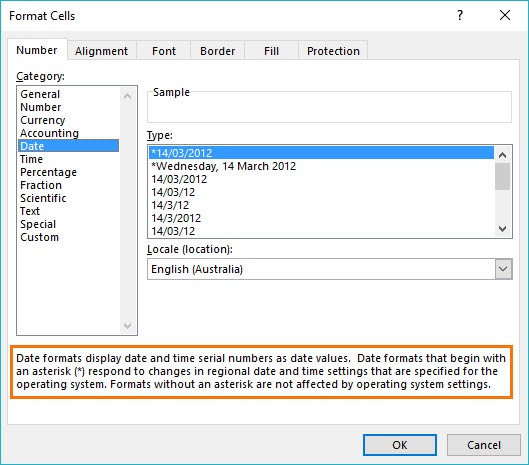
Note: Date formats that begin with an asterisk (*) will change if you change the regional date and time settings in Control Panel. Formats without an asterisk won’t change.
-
If you want to use a date format according to how another language displays dates, choose the language in Locale (location).

Tip: Do you have numbers showing up in your cells as #####? It’s likely that your cell isn’t wide enough to show the whole number. Try double-clicking the right border of the column that contains the cells with #####. This will resize the column to fit the number. You can also drag the right border of the column to make it any size you want.
If you want to use a format that isn’t in the Type box, you can create your own. The easiest way to do this is to start from a format this is close to what you want.
-
Select the cells you want to format.
-
Press CTRL+1.
-
In the Format Cells box, click the Number tab.
-
In the Category list, click Date, and then choose a date format you want in Type. You can adjust this format in the last step below.
-
Go back to the Category list, and choose Custom. Under Type, you’ll see the format code for the date format you chose in the previous step. The built-in date format can’t be changed, so don’t worry about messing it up. The changes you make will only apply to the custom format you’re creating.
-
In the Type box, make the changes you want using code from the table below.
|
To display |
Use this code |
|---|---|
|
Months as 1–12 |
m |
|
Months as 01–12 |
mm |
|
Months as Jan–Dec |
mmm |
|
Months as January–December |
mmmm |
|
Months as the first letter of the month |
mmmmm |
|
Days as 1–31 |
d |
|
Days as 01–31 |
dd |
|
Days as Sun–Sat |
ddd |
|
Days as Sunday–Saturday |
dddd |
|
Years as 00–99 |
yy |
|
Years as 1900–9999 |
yyyy |
If you’re modifying a format that includes time values, and you use «m» immediately after the «h» or «hh» code or immediately before the «ss» code, Excel displays minutes instead of the month.
-
To quickly use the default date format, click the cell with the date, and then press CTRL+SHIFT+#.
-
If a cell displays ##### after you apply date formatting to it, the cell probably isn’t wide enough to show the whole number. Try double-clicking the right border of the column that contains the cells with #####. This will resize the column to fit the number. You can also drag the right border of the column to make it any size you want.
-
To quickly enter the current date in your worksheet, select any empty cell, press CTRL+; (semicolon), and then press ENTER, if necessary.
-
To enter a date that will update to the current date each time you reopen a worksheet or recalculate a formula, type =TODAY() in an empty cell, and then press ENTER.
When you enter some text into a cell such as «2/2″, Excel assumes that this is a date and formats it according to the default date setting in Control Panel. Excel might format it as «2-Feb». If you change your date setting in Control Panel, the default date format in Excel will change accordingly. If you don’t like the default date format, you can choose another date format in Excel, such as «February 2, 2012″ or «2/2/12″. You can also create your own custom format in Excel desktop.
Follow these steps:
-
Select the cells you want to format.
-
Press Control+1 or Command+1.
-
In the Format Cells box, click the Number tab.
-
In the Category list, click Date.
-
Under Type, pick a date format. Your format will preview in the Sample box with the first date in your data.
Note: Date formats that begin with an asterisk (*) will change if you change the regional date and time settings in Control Panel. Formats without an asterisk won’t change.
-
If you want to use a date format according to how another language displays dates, choose the language in Locale (location).
Tip: Do you have numbers showing up in your cells as #####? It’s likely that your cell isn’t wide enough to show the whole number. Try double-clicking the right border of the column that contains the cells with #####. This will resize the column to fit the number. You can also drag the right border of the column to make it any size you want.
If you want to use a format that isn’t in the Type box, you can create your own. The easiest way to do this is to start from a format this is close to what you want.
-
Select the cells you want to format.
-
Press Control+1 or Command+1.
-
In the Format Cells box, click the Number tab.
-
In the Category list, click Date, and then choose a date format you want in Type. You can adjust this format in the last step below.
-
Go back to the Category list, and choose Custom. Under Type, you’ll see the format code for the date format you chose in the previous step. The built-in date format can’t be changed, so don’t worry about messing it up. The changes you make will only apply to the custom format you’re creating.
-
In the Type box, make the changes you want using code from the table below.
|
To display |
Use this code |
|---|---|
|
Months as 1–12 |
m |
|
Months as 01–12 |
mm |
|
Months as Jan–Dec |
mmm |
|
Months as January–December |
mmmm |
|
Months as the first letter of the month |
mmmmm |
|
Days as 1–31 |
d |
|
Days as 01–31 |
dd |
|
Days as Sun–Sat |
ddd |
|
Days as Sunday–Saturday |
dddd |
|
Years as 00–99 |
yy |
|
Years as 1900–9999 |
yyyy |
If you’re modifying a format that includes time values, and you use «m» immediately after the «h» or «hh» code or immediately before the «ss» code, Excel displays minutes instead of the month.
-
To quickly use the default date format, click the cell with the date, and then press CTRL+SHIFT+#.
-
If a cell displays ##### after you apply date formatting to it, the cell probably isn’t wide enough to show the whole number. Try double-clicking the right border of the column that contains the cells with #####. This will resize the column to fit the number. You can also drag the right border of the column to make it any size you want.
-
To quickly enter the current date in your worksheet, select any empty cell, press CTRL+; (semicolon), and then press ENTER, if necessary.
-
To enter a date that will update to the current date each time you reopen a worksheet or recalculate a formula, type =TODAY() in an empty cell, and then press ENTER.
When you type something like 2/2 in a cell, Excel for the web thinks you’re typing a date and shows it as 2-Feb. But you can change the date to be shorter or longer.
To see a short date like 2/2/2013, select the cell, and then click Home > Number Format > Short Date. For a longer date like Saturday, February 02, 2013, pick Long Date instead.
-
If a cell displays ##### after you apply date formatting to it, the cell probably isn’t wide enough to show the whole number. Try dragging the column that contains the cells with #####. This will resize the column to fit the number.
-
To enter a date that will update to the current date each time you reopen a worksheet or recalculate a formula, type =TODAY() in an empty cell, and then press ENTER.
Need more help?
You can always ask an expert in the Excel Tech Community or get support in the Answers community.
Need more help?
-
1
Type the desired date into a cell. Double-click the cell in which you want to type the date, and then enter the date using any recognizable date format. You can enter the date in a variety of different formats.[1]
- Using January 3 as an example, some recognizable formats are «Jan 03,» «January 3», «1/3,» and «01-3.»
-
2
Press the ↵ Enter key. As long as Excel recognizes the date format, it will re-format the cell as a date, which is usually mm/dd/yyyy or dd/mm/yyyy, depending on your locale.
- If the text automatically aligned to the right, then Excel recognized it as a date and re-formatted it.
- If the text stayed aligned to the left, Excel is treating the input as text rather than a date. This could be because it cannot recognize your input as a date, or because that cell’s format is set to something besides a date.
Advertisement
-
3
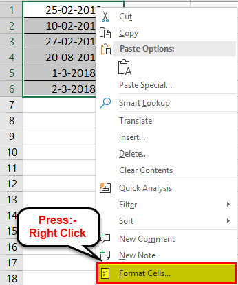
Right-click the date cell and select Format Cells. A new window will pop up.
-
4
Click the Number tab. It’s the first tab.
-
5
Select Date in the «Category» panel. A variety of date formats will appear on the right side of the window.
-
6
Select your desired date format under «Type.» This reformats the selected cell to display in this format.
- You can also change your locale to access date formats used in your location.
-
7
Click OK. The selected cell(s) will now display dates in the selected format.


Advertisement

-
1
Click the cell in which you want today’s date to appear. This can be in an existing formula, or in a new cell.
-
2
Type an equal sign = followed by the formula TODAY(). If you wish to retrieve the current time as well, use NOW() instead of TODAY().[2]
-
3
Hit ↵ Enter. Excel will return today’s date as the cell value. This is a dynamic date, meaning it will change depending on when you are viewing the sheet.
- Use the shortcuts Ctrl + ; and Ctrl + Shift + ; instead to set a cell’s value to today’s date and time respectively as a static value. These values will not update, and act as a timestamp.


Advertisement
-
1
Click the cell in which you want to type the date.
-
2
Type an equal sign = followed by the date formula DATE(year, month, day). Year, month, and day should be numerical inputs.
-
3
Hit ↵ Enter. Excel will return the default date format, which is usually mm/dd/yyyy or dd/mm/yyyy depending on your locale.
-
4
Expand on the formula if required. You can set formulas for the year, month, and day values. Or, you can use the DATE function within other formulas.
- For instance, DATE(2010,MONTH(TODAY()),DAY(TODAY())) sets the cell’s value as today’s month and day in 2010. The formula DATE(2020,1,1)-10 sets the value to 10 days before 1/1/2020.


Advertisement
-
1
Type the desired date into a cell. Double-click the cell in which you want to type the date, and then enter the date using any recognizable date format. You can enter the date in a variety of different formats.
- Using January 3 as an example, some recognizable formats are «Jan 03,» «January 3», «1/3,» and «01-3.»
-
2
Hit ↵ Enter. Excel will re-format the cell and align the text to the right if it has recognized it as a date.
-
3
Select all the cells you wish to fill with dates. Include the cell in which you just entered the date. To select, drag your mouse over all the cells, select an entire column or row, or hold Ctrl (PC) or ⌘ Cmd (Mac) while clicking each cell.
-
4
Click Fill on the Home tab. It’s at the top of Excel in the «Editing» section and looks like a white box with a blue down arrow.
-
5
Click Series…. It is near the bottom.
-
6
Select a «Date unit.» Excel will use this to fill the blank cells based on this setting.
- For instance, if you select «Weekday,» all the blank cells will populate with the weekdays following the initial input date.
-
7
Click OK. Make sure the are dates filled in correctly.


Advertisement
Ask a Question
200 characters left
Include your email address to get a message when this question is answered.
Submit
Advertisement
-
Set a custom date format in Excel by right-clicking a cell, clicking Format Cells, and selecting «Custom» as the category in the Number tab. Review the available date options. Create your own by typing the format code using an existing code.
Advertisement
References
About This Article
Article SummaryX
1. Click on a cell.
2. Type in a date.
3. Hit Enter.
4. Review the date format. Change by right-clicking and selecting Format Cells.
Did this summary help you?
Thanks to all authors for creating a page that has been read 12,928 times.
Is this article up to date?
This article will explain to you how to change the default Date format by your custom display.
How is displayed a date in Excel?
By default, when you insert a date in a cell, the default delimiter between the day, the month and the year it’s the slash. And this, even if you write your date with dashes.
Excel automatically replaces the dashes with slashes 🤔

Change the default Date format
If you want to customize the default display, you must change a Windows setting.
Step 1: Open the Regional setting
To open the Regional setting quickly, you write the command line intl.cpl in the Windows Search box

And there, you have the following dialog box with the default date format.

Step 2: Select another date format
When you press on the drop-down button, you display other date formats but the number of choices is limited 😕

Step 3: Change the default date format
To change the default date format, you must click on the button Additional Settings

Step 4: Create your custom date format
- Select the Date tab
- Change the custom date format (here dd-MM-yyyy)

The code of your custom date follow the standard rules of date format in Excel
And without restarting Excel, neither your computer, all the dates format in your worksheets has the dash for date delimiter 😉

Caution
When you change the setting of the date format of Windows, ALL THE DATES of your computer are impacted.
As you can see, after changing the default date format, the format of the date in the taskbar has changed too.

The objective of this post is to teach you how Excel handles date and time and provide you with all the tools you will need.
It’s designed to be read in conjunction with the accompanying Excel file, which you can download below.
Download the Files
Enter your email address below to download the comprehensive Excel workbook and PDF.
By submitting your email address you agree that we can email you our Excel newsletter.
Regional Settings
When reading this post keep in mind that my regional settings format dates as dd/mm/yyyy and so the screenshots throughout this post are in this format. However, if you open the accompanying Excel file you may see some dates have switched to match your regional settings, which may be different to mine e.g. mm/dd/yyyy.
Dates and times with a format that begins with an asterisk (*) automatically update based on your PC’s regional settings. You can see an example in the Format Cells dialog box below:
Ok, let’s crack on.
Excel Date and Time 101
Excel stores dates and time as a number known as the date serial number, or date-time serial number.
When you look at a date in Excel it’s actually a regular number that has been formatted to look like a date. If you change the cell format to ‘General’ you’ll see the underlying date serial number.
The integer portion of the date serial number represents the day, and the decimal portion is the time. Dates start from 1st January 1900 i.e. 1/1/1900 has a date serial number of 1.
Caution! Excel dates after 28th February 1900 are actually one day out. Excel behaves as though the date 29th February 1900 existed, which it didn’t.
Microsoft intentionally included this bug in Excel so that it would remain compatible with the spreadsheet program that had the majority market share at the time; Lotus 1-2-3.
Lotus 1-2-3 was incorrectly programmed as though 1900 was a leap year. This isn’t a problem as long as all your dates are later than 1st March 1900.
Excel gives each date a numeric value starting at 1st January 1900. 1st January 1900 has a numeric value of 1, the 2nd January 1900 has a numeric value of 2 and so on. These are called ‘date serial numbers’, and they enable us to do math calculations and use dates in formulas.
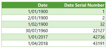
The Date Serial Number column displays the Date column values in their date serial number equivalent.
e.g. 1/1/2017 has a date serial number of 42736. i.e. 1st January 2017 is 42,736 days since 31st December 1899.
Tip: format the date serial number column as a Date and you’ll see they look the same as the Date column values.
Time
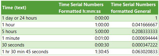
Times also use a serial number format and are represented as decimal fractions.
Hours: since 24 hours = 1 day, we can infer that 24 hours has a time serial number of 1, which can be formatted as time to display 24:00 or 12:00 AM or 0:00. Whereas 12 hours or the time 12:00 has a value of 0.50 because it is half of 24 hours or half of a day, and 1 hour is 0.41666′ because it’s 1/24 of a day.
Minutes: since 1 hour is 1/24 of a day, and 1 minute is 1/60 of an hour, we can also say that 1 minute is 1/1440 of a day, or its time serial number is 0.00069444′
Seconds: since a second is 1/60 of a minute, which is 1/60 of an hour, which is 1/24 of a day. We can also say one second is 1/86400 of a day or in time serial number form it’s 0.0000115740740740741…
Date & Time Together
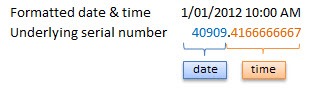
Now that we know how dates and times are stored we can put them together — ddddd.tttttt
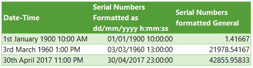
For example, the date and time of 1st January 2012 10:00:00 AM has a date-time serial value of 40909.4166666667
40909 being the serial value representing the date 1st January 2012, and .4166666667 being the decimal value for the time 10:00 AM and 00 seconds.
More examples below.
Entering Dates & Times in Excel
Entering Dates
You can type in various configurations of a date and Excel will automatically recognise it as a date and upon pressing ENTER it will convert it to a date serial number and apply a date format on the cell.
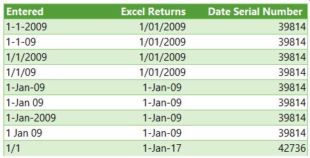
For example, try typing (or even copy and paste) the following dates into an empty cell:
| 1-1-2009 |
| 1-1-09 |
| 1/1/2009 |
| 1/1/09 |
| 1-Jan-09 |
| 1-Jan 09 |
| 1-Jan-2009 |
| 1 Jan 09 |
| 1/1 |
You can see in the table above that entering numbers that look like dates and are separated by a forward slash or hyphen will be recognised as a date. Even typing in a date with the month name gets converted to a date.
However, dates separated with a period like this 1.1.2009, or with spaces between numbers like this 01 01 2009, will end up as text, not a date. Gotta have some limits!
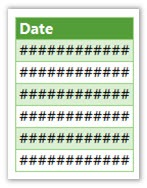
Tip: Dates that display ##### in a cell usually indicate that the column is simply not wide enough to display it.
However, if you make the cell really wide and it still displays ##### then this indicates that the date is a negative value and Excel can’t display negative dates.
Entering Dates with Two Digit Years
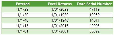
When you enter a date with two digits for the year e.g. 1/1/09, Excel has to decide if you mean 2009 or 1909.
It goes by the rule that dates with years 29 or before, are treated as 20xx and dates with the year 30 or older are treated as 19xx. See examples below.
Tip: You can enter the day and month portions of a date and Excel will insert the year based on your computer’s clock. Nice to know for data entry.
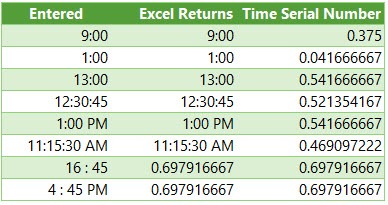
Entering Time
When you enter time you must follow a strict format of at least h:mm. i.e. the hour and minutes are separated by a colon with no spaces either side. Entering the h:mm components will result in a time formatted in military time e.g. 2:00 PM is 14:00 in military time.
If you enter a time that includes a seconds component e.g. 3:15:40, Excel will automatically format the cell in h:mm:ss.
If you want the time to be formatted with AM/PM you can simply enter a space after the time and then type AM or PM, or apply the number format to the cell later. Here are some examples:
Entering Dates & Time Together
Now that we know how to enter dates and time separately we can put them together to enter a date and time in the same cell.
You can even enter time then date and Excel will fix the order for you.
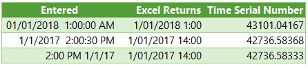
You’ll find that even if you enter AM/PM, that Excel will convert it to military time by default. You can override this with a custom number format. More on that later.
Simple Date & Time Math
Now that we understand that Excel stores dates and time as serial numbers, you’ll see how logical it is to perform math operations on these values. We’ll look at some simple examples here and tackle the more complex scenarios later when we look at Date and Time Functions.
Adding/Subtracting Days from Dates
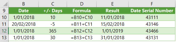
Tip: you can also add/subtract the days directly in the formula e.g. =B10+10 or =B11-5 Although, it’s better to place the values you’re adjusting by in their own cell or a named range.
Subtracting Dates from one another
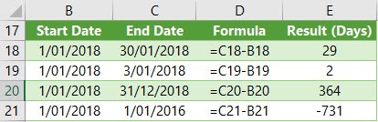
Tip: format the cell to General or Number to see the number of days between two dates.
Note: the ‘result’ is exclusive of the start day i.e. it assumes the start day is at the end of that day.
Adding Times to one another
The time being added is input as a time serial number. Notice there are no negative times in the table below. Remember we can’t display negative times. Instead we need to use the math operator to tell Excel to subtract time. See examples below.
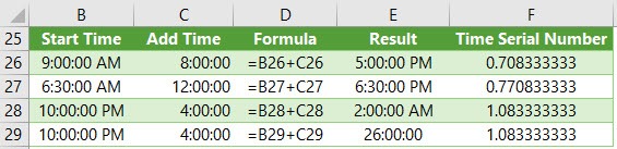
Note: Times that roll over to the next day result in a time-date serial number >= 1. Cell E28 actually contains a time-serial number of 1.08333′, but since the cell is formatted to display time formatted as h:mm:ss, only the time portion is visible.
If you want to show the cumulative time (like cell E29) then you need to surround the ‘h’ part of the time format in square brackets like so: [h]:mm:ss
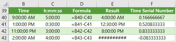
Subtracting Time from Times
Notice the last result in the table below shows ######, this is because it results in a negative time and Excel can’t display that, but notice it can return a negative time serial number. More on how to solve this later.
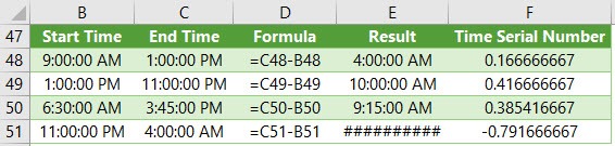
Subtracting Times from one another
Again, here the last result shows ###### because it results in a negative time.
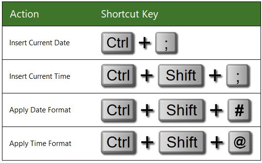
Excel Date and Time Shortcuts
‘Good to Know’ Stuff about Excel Date and Time
— Dates prior to 1st January 1900 are not recognised in Excel.
— A negative date will display in the cell as #######
— Times stored without a date effectively inherit the date 0 Jan 1900 i.e. the month is Jan and the year 1900 and the day is zero. Remember, there are no dates prior to 1/1/1900 from Excel’s perspective. This means that times stored without a date e.g. 0.50 for 12:00 PM is the equivalent of 0 Jan 1900 12:00 PM.
This is important because if you try to take 14 hours from 12 hours (without a date) you’ll get the dreaded ###### display in the cell, because negative dates and times cannot be displayed. We’ll cover workarounds for this later, but for now keep in mind that math on dates and time that result in negative date-time serial numbers cannot be formatted as a date.
Date Modes
— Excel actually has two date modes. The other mode is called 1904 Date System and is used for compatibility with Excel 2008 for Mac and earlier Mac versions. You can change the date system in the Advanced Options.
In the 1904 date system dates are calculated using 1st January 1904 as the starting point. The difference between the two date systems is 1,462 days. This means that the serial number of a date in the 1900 date system is always 1,462 days greater than the serial number of the same date in the 1904 date system. 1,462 days is equal to four years and one day (including one leap day).
Caution; the date setting you choose applies to all dates within the workbook. You can’t mix and match modes and you shouldn’t reference workbooks that use a different date system in formulas.
Bottom line; don’t use the 1904 date system unless absolutely necessary! Click here for more on date systems in Excel.
— Excel applies date number formats based on your system region settings. For example, my system is set to display dates in dd/mm/yyyy format, but if you’re in the U.S. your system is likely to format them as mm/dd/yyyy. Excel will automatically convert the format of date serial numbers to suit your system settings as long as it’s one of the default date formats and not a custom number format.
More Excel Date and Time Tips
This post is just the beginning, the next steps in mastering Excel Date and Time are below:
- Every Excel Date and Time Function explained
- Formatting Date and Time in Excel
- Common Date and Time Calculations
Tip: Avoid waiting, download the workbook and get the above topics now.
Enter your email address below to download the comprehensive Excel workbook and PDF.
By submitting your email address you agree that we can email you our Excel newsletter.
When you enter a date into Microsoft Excel, the program will format it according to the default date settings. For example, if you want to enter the date February 6, 2020, the date could appear as 6-Feb, February 6, 2020, 6 February, or 02/06/2020, all depending on your settings. You may find that if you change a cell’s formatting to “Standard,” your date becomes stored as integers. For example, February 6, 2020 would become 43865, because Excel bases date formatting off of January 1, 1900. Each of these options are ways to format dates in Excel. To help with organizing data in Excel, learn about how to change the date format in Excel.
Choosing from the Date Format List
Formatting dates in Excel is easiest with the date formats list. Most date formats you may want to use can be found in this menu.
How to Change The Excel Date Format
- Select the cells you want to format
- Click Ctrl+1 or Command+1
- Select the “Numbers” tab
- From the categories, choose “Date”
- From the “Type” menu, select the date format you want

Creating a Custom Excel Date Format Option
To customize the date format, follow the steps for choosing an option from the date format list. Once you’ve selected the closest date format to what you want, you can customize it and change it.
- In the “Category” menu, select “Custom”
- The type you chose earlier will appear. The changes you make will only apply to your customized setting, not to the default
- In the “Type” box, enter the correct code to alter the date
- If you are trying to change the date display to DD/MM/YYYY, simply go to Format Cells > Custom
- Next, Enter DD/MM/YYYY in the available space given.

Converting Date Formats to Other Locales
If you are using dates for several different locations, you might need to convert to a different locale:
- Select the right cell or cells
- Hit Ctrl+1 or Command+1
- From the “Numbers” menu, select “Date”
- Underneath the “Type” menu, there’s a drop-down menu for “Locale”
- Select the right “Locale”

You can also customize the locale settings:
- Follow the steps for customizing a date
- Once you’ve created the right date format, you need to add the locale code to the front of the customized date format
- Choose the right locale codes. All locale codes are formatted as [$-###]. Some examples include:
- [$-409]—English, United States
- [$-804]—Chinese, China
- [$-807]—German, Switzerland
- Find more locale codes

Tips for Displaying Dates in Excel
Once you have the right date format, there are additional tips to help you figure out how to organize data in Excel for your datasets.
- Make sure the cell is wide enough to fit the entire date. If the cell isn’t wide enough, it will display #####. Double click on the right border of the column to make your column expand enough to display the date correctly.
- Change the date system if negative numbers appear as dates. Sometimes Excel will format any negative numbers as a date because of the hyphens. To fix this, select the cells, open the options menu, and select “Advanced.” On that menu, select “Use 1904 date system.”
- Use functions to work with today’s date. If you want a cell to always display the current date, use the formula =TODAY() and press ENTER.
- Convert imported text to dates. If you import from an external database, Excel will automatically register the dates as text. The display may look the same as if they were formatted as dates, but Excel will treat the two differently. You can use the DATEVALUE function to convert.
Why Your Date Format May Not Be Having Issues Changing
There are many reasons why you might be experiencing issues changing the date format in Excel. Listed are a few common difficulties.
- There could be text in the column, not dates (which are actually numbers).
- Dates are left-aligned
- An apostrophe could be included in the date
- A cell may be too wide.
- Negative numbers are formatted as dates
- Excel TEXT function is not being utilized.
Even with correctly formatted dates and displays, organizing data in Excel can only work as well as the data does. Messy data won’t lead to insights during analysis, however, it’s formatted.
Data Preparation with Excel
Formatting data, by doing things like formatting dates, is part of a larger process known as “data preparation,” or all of the steps required to clean, standardize, and prepare data for analytic use.
While data preparation is certainly possible in Excel, it becomes exponentially more difficult as analysts work with larger and more complex datasets. Instead, many of today’s analysts are investing in modern data preparation platforms like Designer Cloud to accelerate the overall data preparation process for data big or small.
Schedule a demo of Designer Cloud to see how it can improve your data preparation process, or try the platform for yourself by getting started with Designer Cloud today.
What is the Date Format in Excel?
In Excel, a date is displayed according to the format selected by the user. One can choose from the different formats available or create a customized format according to the requirement. The default date format is specified in the “Control Panel” of the system. However, it is possible to change these default settings.
For example, the date 01/01/2021 corresponds to the format dd/mm/yyyy. If the format is changed to d-mmm-yyyy, the date becomes 1-Jan-2021.
We can change the date format in Excel either from the “Number Format” of the “Home” tab or the “Format Cells” option of the context menu.
In Excel for Windows, 1900 is the default date system. Whereas, in Excel for Mac, 1904 is the default date system. Both these systems store the dates as consecutive numbers having a difference of 1. These numbers are known as serial values or serial numbers. The reason dates are stored as serial numbers is to facilitate calculations.
In the 1900 date system, the first date that Excel recognizes is January 1, 1900. This date is stored as the number 1 in Excel. Consequently, the number 2 represents January 2, 1900. The last date recognized by Excel is December 31, 9999. It is represented by the serial number 2958465. Date before 1900 or after 9999 is identified as a text value by Excel.
Dates are stored only as positive integers in the 1900 date system. However, to display negative numbers as negative dates, one needs to switch to the 1904 date system.
In the 1904 date system, 0 represents January 1, 1904, and -1 means January -2, 1904. The number 1 represents January 2, 1904. The last date recognized by Excel (in the 1904 date system) is December 31, 9999, represented by the serial number 2957003.
In this article, we follow the 1900 date system.
Table of contents
- What is theDate Format in Excel?
- Code of Date Format in Excel
- How to Change Date Format in Excel?
- Example #1–Apply Default Format of Long Date in Excel
- Example #2–Change the Date Excel Format Using “Custom” Option
- Example #3–Apply Different Types of Customized Date Formats in Excel
- Example #4–Convert Text Values Representing Dates to Actual Dates
- Example #5–Change the Date Format Using “Find and Replace” Box
- Frequently Asked Questions
- Recommended Articles
Code of Date Format in Excel
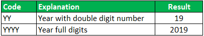
A code (like dd-mm-yyyy) is a representation of a day (d), month (m), and year (y). We can change the appearance of the date by changing the specified code.
The different codes, their explanation, and output (for days, months, and years) have been presented in the following images.
Notations for a Day

Notations for a Month

Notations for a Year
How to Change Date Format in Excel?
Here we look at some of the date format examples in Excel and how to change them.
Example #1–Apply Default Format of Long Date in Excel
The following image shows a number in cell A1. We want to know the date represented by this number. The output should be in the long date format of Excel.
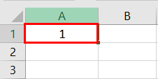
The steps to know the date represented by the number in cell A1 are listed as follows:
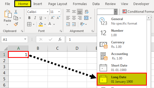
- We must first select cell A1. Then, from the “Home” tab, click the “Number Format” drop-down appearing in the “Number” section. Next, select “Long Date,” shown in the following image.

- The output is shown in the following image. The long date format displayed is dd mmmm yyyy. Hence, the number 1 represents the date 01 January 1900 in the long date format.
Note: The short and long dates appear as set in the “Control Panel.” Click “Clock, Language, and Region” in the “Control Panel” to change these default date formats. After that, click “Change date, time, or number formats.” Make the desired changes and click “OK.”
Likewise, had there been 2 in cell A1, the long date format would have been 02 January 1900. The number 3 would have been displayed as 03 January 1900 in the long date format.
Note: To switch to the 1904 date system, we must select “Advanced” from the “Options” of the “File” tab. Under “When calculating this workbook,” select “use 1904 date system” and click “OK.”

You can download this Change Date Format Excel Template here – Change Date Format Excel Template
Example #2–Change the Date Excel Format Using “Custom” Option
The following image shows some dates in the range A1:A6. These dates are in the format dd-mm-yyyy. We want to change their format to dd-mmmm-yyyy.
For instance, the date in cell A1 should appear as 25-February-2018. We may use the “Custom” option of the “Format Cells” dialog box.

The steps to change the date format in Excel are listed as follows:
Step 1: We need to select all the dates of the range A1:A6. The same is shown in the following image.
Step 2: We must right-click the selection and choose “Format Cells” from the context menu. Alternatively, we may also press the keys “Ctrl+1” together.
Step 3: The “Format Cells” window opens, as shown in the following image.
Note: The default short date and long date formats are marked with an asterisk (*) in the box under “type.” The short date is 3/14/2012 (m/dd/yyyy), and the long date is Wednesday, March 14, 2012 (dddd, mmmm dd, yyyy).
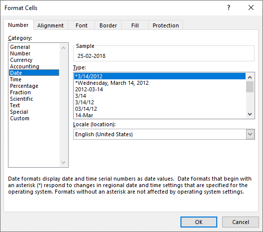
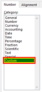
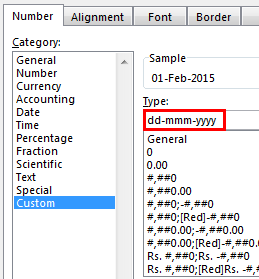
Step 4: From the “Number” tab, we need to select “Custom” under “Category.” The categories are shown on the left side of the “Format Cells” window.
Step 5: Under “Type,” we must insert the required date format. Either type the format (dd-mmmm-yyyy) or select it from the various options displayed in the box below “Type.”
Once the format has been entered, check the preview of the first date (of the range A1:A6) under “Sample.” The same is shown in the following image. Click “OK” in the “Format Cells” window if the date preview looks good.
Note 1: The date under “Sample” is displayed according to the format specified under “Type.”
Note 2: While creating custom date formats, we can use a forward slash (/), hyphen (-), comma (,), space ( ), etc.

Step 6: The output is shown in the following image. All dates of the range A1:A6 have been converted to the format dd-mmmm-yyyy. However, the Excel formula bar can still see the default date format. This default format corresponds with the short date set in the “Control Panel.”

Example #3–Apply Different Types of Customized Date Formats in Excel
The next image shows certain dates in the range A1:A6. At present, the date format is dd-mm-yyyy.
We want to apply four different formats to these dates. For using each format, the common steps to be performed are given as follows:
- First, we must select the range A1:A6.
- Then, right-click the selection and choose “Format Cells.”
- After that, from the “Number” tab, select “Custom” under “Category.”
Further, under each format, the additional steps to be performed followed by two images are given.

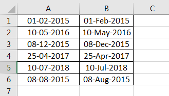
Format 1: dd-mmm-yyyy
- In the “Custom” option of the “Number” tab, select the format “dd-mmm-yyyy” under “Type.”
- Click “Ok.”

The output is given in the following image. All dates are displayed according to the format dd-mmm-yyyy. The hyphen is the separator between the day, month, and year in this format.

Format 2: dd mmm yyyy
- We must select the format “dd mmm yyyy” under “Type” of the “custom” option.
- Click “Ok.”

The output is given in the following image. All dates are converted to the format dd mmm yyyy. The space is the only separator between the day, month, and year in this format.

Format 3: ddd mmm yyyy
- In the “Custom” option, select the format “ddd mmm yyyy” under “Type.”
- Click “Ok.”

The output is given in the following image. The dates are shown in the format ddd mmm yyyy. The day and the month are displayed in their short notations in this format.

Format 4: dddd mmmm yyyy
- From the “Custom” option of the “Number” tab, select “dddd mmmm yyyy” under “Type.”
- Click “Ok.”

The output is given in the following image. All dates have been converted to the format dddd mmmm yyyy. The date, month, and year are displayed in their respective full forms in this format.

It must be observed that the date format changes as per the style set by the user. Therefore, the user can select a date format according to their convenience.
Example #4–Convert Text Values Representing Dates to Actual Dates
The following image shows a list of dates in the range A1:A6. At present, these dates are appearing as text values. We want to convert these text values to dates having the format dd-mmm-yyyy.

The steps to convert text values to dates having the given format are listed as follows:
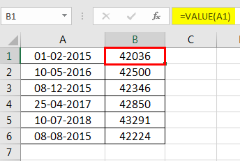
Step 1: First, enter the following formula in cell B1.
“=VALUE(A1)”
Then, press the “Enter” key.
Note 1: The VALUE functionIn Excel, the value function returns the value of a text representing a number. So, if we have a text with the value $5, we can use the value formula to get 5 as a result, so this function gives us the numerical value represented by a text.read more returns the numeric form of a text string that represents a number. In other words, it converts a number looking like the text into an actual number.
Note 2: Instead of the VALUE function, one can also use the DATEVALUE functionThe DATEVALUE function in Excel shows any given date in absolute format. This function takes an argument in the form of date text normally not represented by Excel as a date and converts it into a format that Excel can recognize as a date.read more of Excel. The latter converts a date stored as text to a serial number. This serial number is recognized as a date by Excel.
Step 2: We must select cell B1 and drag the fill handle until cell B6. The output is shown in the following image. All text values (A1:A6) have been converted to numbers (in the range B1:B6).
Ideally, the text string in Excel is left-aligned while the number string is right-aligned. However, we have centrally aligned both the ranges (A1:A6 and B1:B6).
Note: When text strings representing dates have been converted to serial values (or dates), we can use them for performing different calculations like addition, subtraction, and so on.
Step 3: To view the obtained serial numbers (in column B) as dates, apply the required format. We must select the range B1:B6, right-click and choose “Format Cells.”
In the “Number” tab, select the option “Custom.” Then, under “Type,” enter or choose the format “dd-mmm-yyyy.” The same is shown in the following image.
If the sample date looks alright, click “OK.”
Step 4: The output is shown in the following image. Hence, all text values (of column A) have been converted to valid dates (in column B) having the format dd-mmm-yyyy.
Note: To ensure that a value is recognized as a date by Excel, check for the following signs:
- The dates are right-aligned as they are numerical values.
- If two or more dates are selected, the status bar (at the bottom of the worksheet) shows the count, average, numerical count, and sum. In addition, it may display one or more options according to the Excel version.
If a value is a text string, it would be left-aligned, and the status bar will show only the count.
Often, the Excel date format needs to be changed (from text to dates) when data is downloaded (or copied and pasted) from the web. That is because, in such instances, the dates may not be displayed as numbers.
Example #5–Change the Date Format Using “Find and Replace” Box
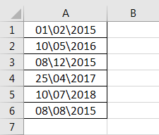
The following image shows some text values representing dates in the range A1:A6. The days, months, and numbers have been separated with a backslash. That is because we want to perform the following tasks:
- Replace all the backslashes () with forwarding slashes (/) by using the “Find and Replace” dialog box.
- Convert text values representing dates to actual dates.
The steps to perform the given tasks are listed as follows:
Step 1: We must press the keys “Ctrl+H” together. Then, the “find and replace” dialog box opens, as shown in the following image.
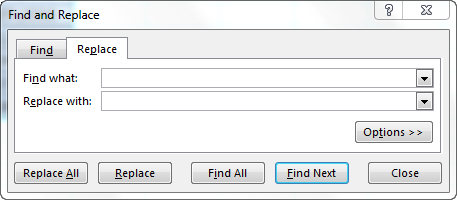
Step 2: Type a backslash in the “Find what” box (). In the “Replace with” box, type a forward slash (/).
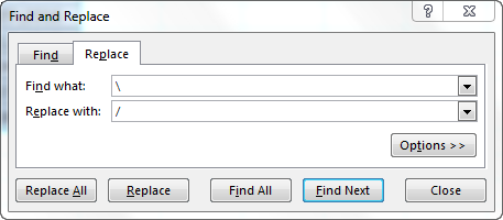
Step 3: Next, we must click “Replace All.” Excel shows a message stating the number of replacements it has made. Click “OK” to proceed. The final output is shown in the following image.
Hence, all backslashes have been replaced with forwarding slashes. With this replacement, the text values representing dates have automatically been converted to actual dates by Excel.
Since column A was aligned centrally from the beginning, this alignment is retained even after the values are converted to dates.

Frequently Asked Questions
1. How can the date format in Excel be changed?
The steps to change the date format in Excel are listed as follows:
The steps to change the date format in Excel are listed as follows:
a. Select the cell containing the date. If the date format of a range needs to be changed, select the entire range.
b. Right-click the selection and choose “Format Cells” from the context menu. Alternatively, press the keys “Ctrl+1” together.
c. IIn the “Number” tab, select the option “Date.” Next, select the required date format under “Type.”
d. Check the preview (of the first date of the selected range) under “Sample.” If the preview is good, click “OK.”
The date format of the selected cell or cells (selected in step a) is changed.
Note 1: The required date format may not be available under the “Date” option’s “Type.” If it is not available, select “Custom” as the “category” from the “Number” tab. Then, type the required date format under “Type” and click “OK.”
Note 2: If the selected cell (selected in step a) contains a text string representing a date, convert this string to date first. Then change the format to the desired date format.
2. How to change the date format permanently in Excel?
To change a date format permanently, one needs to make changes to the date formats of the “Control Panel.” That is because the short and long date formats of Excel reflect the date settings of the “Control Panel.”
The steps to change the date settings of the “Control Panel” are listed as follows:
We must open the “Control Panel” first from the “Start” menu.
b. In the “Clock, Language, and Region” category, click “Change date, time, or number format.” It is available under the “Region and Language” option.
c. The “Region and Language” or “Region” dialog box opens. Under “Format,” we must select the region.
d. Enter the required short and long date formats under “Date and Time Formats.” To enter customized short and long date formats, click “Additional Settings.” The “Customize Format” dialog box opens. Make the changes in the “Date” tab and click “OK.”
e. Check the preview under “Examples” at the bottom of the “Region and Language” box. If the preview is alright, click “OK.”
The default date settings have been changed. Now, we should enter a date in any format in Excel. Then select the short or the long date format from the “Number Format” (in the “Number” section) of the “Home” tab.
The dates will appear in the format set in the “Control Panel.” So, the user need not change the format of each date manually.
3. How to change a date to a text string in Excel?
Let us change the date 22/1/2019 in cell A1 to a text string in Excel. The text string should be in the format yyyy-mm-dd.
The steps to change a date to a text string are listed as follows:
a. First, we must enter the formula =TEXT(A1, “yyyy-mm-dd”) in cell B1.
b. Then, press the “Enter” key.
The date in cell A1 (22/1/2019) is converted to 2019-01-22 in cell B1. We must note that the date in cell A1 is right-aligned, being a number. In contrast, the text in cell B1 is left-aligned.
Note: The TEXT function helps convert numbers to text strings. It is used to display values in a specific format. The syntax is TEXT(value,format_text). “Value” is the number to be converted to text. “Format_text” is the format in which the number should be displayed.
Recommended Articles
This article has been a guide to the Date Format in Excel. We discuss changing and customizing date formats in Excel, practical examples, and a downloadable Excel template. You may also look at these useful functions in Excel: –
- Concatenate Columns in Excel
- Convert Date to Text in Excel
- Insert Date in Excel
- Concatenate Date in Excel
 Dates and times are two of the most common data types people work with in Excel, but they are also possibly the most frustrating to work with, especially if you are new to Excel and still learning. This is because Excel uses a serial number to represent the date instead of a proper month, day, or year, nevermind hours, minutes, or seconds. It’s made more complicated by the fact that dates are also days of the week, like Monday or Friday, even though Excel doesn’t explicitly store that information in the cells. Here is the definitive guide to working with dates and times in Excel…
How Excel Stores Dates
The source of most of the confusion around dates and times in Excel comes from the way that the program stores the information. You’d expect it to remember the month, the day, and the year for dates, but that’s not how it works…
Excel stores dates as a serial number that represents the number of days that have taken place since the beginning of the year 1900. This means that January 1, 1900 is really just a 1. January 2, 1900 is 2. By the time we get all the way to the present decade, the numbers have gotten pretty big… September 10, 2013 is stored as 41527.
Importantly, any date before January 1, 1900 is not recognized as a date in Excel. There are no “negative” date serial numbers on the number line.
It seems confusing, but it makes it a lot easier to add, subtract, and count days. A week from September 10, 2013 (September 17, 2013), is just 41527 + 7 days, or 41534.
How Excel Stores Times
Excel stores times using the exact same serial numbering format as with dates. Days start at midnight (12:00am or 0:00 hours). Since each hour is 1/24 of a day, it is represented as that decimal value: 0.041666…
That means that 9:00am (09:00 hours) on September 10, 2013 will be stored as 41527.375.
When a time is specified without a date, Excel stores it as if it occurred on January 0, 1900. In other words, 3:00pm (15:00 hours) is stored as 0.625. This can make doing math for time-only values (that have no date) challenging, since subtracting 6 hours (6:00) from 3:00am (03:00 hours) will become negative and count as an error: 0.125 – 0.25 = -0.125, which is displayed as #########.
Minutes and seconds in Excel work the same way as hours…
A minute is 1/60 of an hour, which is 1/24 of a day, or 1/1440 of a day in total, which calculates to 0.00069444…
A second is 1/60 of an minute, which is 1/60 of an hour, which is 1/24 of a day, or 1/86400 of a day in total, which calculates to 0.00001157407…
Working with Dates and Times
DATE() and TIME()
Serial numbers aren’t all that intuitive to use. Fortunately, Excel has a set of functions to make it easier to find and use dates and times, starting with DATE and TIME. The syntax is as follows:
=DATE(year, month, day)
=TIME(hours, minutes, seconds)
For both functions, specify the year, month, and day, or hours, minutes, and seconds as numbers. For example, September 10, 2013 can be entered as:
=DATE(2013,9,10)
It will be stored as 41527, which means that it is technically storing 12:00am on September 10, 2013.
For times, 6:00pm (18:00 hours) can be entered as:
=TIME(18,0,0)
It will be stored as 0.75, which means that it is technically storing 6:00pm on January 0, 1900.
If we want to represent a specific time and date, we can add the two functions together. For example, 6:00pm (18:00 hours) on September 10, 2013 can be entered as:
=DATE(2013,9,10)+TIME(18,0,0)
It will be calculate as 41527.75, which means Excel is storing exactly the date we want…
Additional Date and Time Setting Functions
Excel has a few additional functions to make declaring dates easier.
TODAY()
The TODAY function always returns the current date’s serial number. The TODAY function is just entered as:
=TODAY()
This article was written at 6:30pm (18:30 hours) on September 24, 2013, and the TODAY function calculated to 41541. That means that it is technically storing 12:00am on September 24, 2013.
NOW()
A similar function called NOW always returns the current date and time’s serial number. The NOW function is just entered as:
=NOW()
Again, at 6:30pm (18:30 hours) on September 24, 2013, the function calculated to 41541.77081333… NOW stores the exact time and date, down to the second.
EDATE() and EOMONTH()
The EDATE function gives the date the specified number of months away from the input date. The EOMONTH function gives the date of the last day of the month. It can do so for the current month or a number of months in the future or the past. The syntax for each is as follows:
=EDATE(start_date, months)
=EOMONTH(start_date, months)
The start_date can be any date-formatted cell reference or date serial number.
The months field can be any number, though only the integer value will be used (e.g. it treats 2.8 as 2).
The EDATE and EOMONTH functions strip the time value from the date. For example, For example, if cell A1 stores September 10, 2013, we can get the value 2 months ahead as follows:
=EDATE(A1,2)
Returns 12:00am (0:00 hours) on November 10, 2013, or 41588. This function works even though the months have different numbers of days (September and November have 30, October has 31).
=EOMONTH(A1,2)
Returns 12:00am (0:00 hours) on November 30, 2013, or 41588. Again, this function works even though the months have different numbers of days.
WORKDAY()
Occasionally, it may be useful to count ahead based on work-days (Monday-Friday) instead of all 7 days of the week… For that, Excel has provided WORKDAY. The syntax for WORKDAY is as follows:
=WORKDAY(start_date, days, [holidays])
The start_date is as above.
The days input is the number of workdays ahead (or behind) of the present day you would like to move.
The [holidays] input is optional, but lets you disqualify specific days (like Thanksgiving or Christmas, for example), which might otherwise fall during the work week. These are date serial numbers provided in an array bounded by brackets: { }. To specify multiple holidays, the dates must be held in cells – it is not possible to put multiple DATE functions in an array.
For example, let’s find the date 6 work days before 6:00pm (18:00 hours) on September 10, 2013 (stored in cell A1). Monday, September 2nd is Labor Day, so let’s include that as a holiday:
=WORKDAY(A1,-6,DATE(2013,9,2))
Returns 12:00am (0:00 hours) on August 30, 2013, or 41516. (Note that the function strips the time portion of the date.)
WORKDAY.INTL() (Excel 2010 and newer)
For newer versions of Excel (2010 and later), there is another version of WORKDAY called WORKDAY.INTL. WORKDAY.INTL works just like WORKDAY, but it adds the ability to customize the definition of the “weekend”. The syntax for WORKDAY.INTL is as follows:
=WORKDAY.INTL(start_date, days, [weekend], [holidays])
The start_date, days, and [holidays] inputs work just like the normal WORKDAY function.
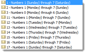
The [weekend] input has the following options:
Retrieving Dates in Excel
DAY(), MONTH(), and YEAR()
Now we know how define dates, but we still need to be able to work with them. Serial numbers don’t make it easy to extract months, years, and days, nevermind hours, minutes, and seconds. That’s why Excel has specific functions for pulling out each of these values. For working with the calendar, there is DAY, MONTH, and YEAR. The syntax is simple:
=DAY(serial_number)
=MONTH(serial_number)
=YEAR(serial_number)
The serial_number in each can be any date-formatted cell reference. For example, if cell A1 stores September 10, 2013, we can use each of the formulas in turn:
=DAY(A1)
Returns 10 as a numeric value.
=MONTH(A1)
Returns 9 as a numeric value.
=YEAR(A1)
Returns 2013 as a numeric value.
We could have also given the direct serial number for September 10, 2013:
=DAY(41527)
Returns 10 as a numeric value.
Retrieving Times in Excel
HOUR(), MINUTE(), and SECOND()
For times, the process is very similar. Excel has function to retrieve the hours, minutes, and seconds from a time stamp, conveniently named HOUR, MINUTE, and SECOND. The syntax is identical:
=HOUR(serial_number)
=MINUTE(serial_number)
=SECOND(serial_number)
The serial_number in each can be any time/date-formatted cell reference. For example, if A1 stores 6:15:30pm (18:15 hours, 30 seconds) on September 10, 2013, we can use each of the formulas in turn:
=HOUR(A1)
Returns 18 as a numeric value.
=MINUTE(A1)
Returns 15 as a numeric value.
=SECOND(A1)
Returns 30 as a numeric value.
We could have also given the direct serial number for 6:15:30pm (18:15 hours, 30 seconds) on September 10, 2013:
=SECOND(41527.7607638889)
Returns 30 as a numeric value.
Additional Date Retrieving Functions
WEEKDAY() and WEEKNUM()
Dates don’t just have month and year information. They also encode indirect information… September 10, 2013 happens to also be a Tuesday. Excel has a few of functions to work with the week aspect of dates: WEEKDAY and WEEKNUM. The syntax is as follows:
=WEEKDAY(serial_number, [return_type])
=WEEKNUM(serial_number, [return_type])
The serial_number in each can be any date-formatted cell reference. Since [return_type] is optional, each function assumes that each week starts on Sunday. If cell A1 stores September 10, 2013 (a Tuesday), we can use each of the formulas in turn:
=WEEKDAY(A1)
Returns 3, since Tuesday is the 3rd day of a week that starts on Sunday.
=WEEKNUM(A1)
Returns 37, since September 10, 2013 is in the 37th week of 2013, when you start counting weeks from Sunday.
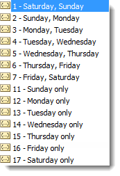
The [return_type] allows you to specify a different default week arrangement. You could let the week start on Monday and run until Sunday, or Saturday until Friday, for example. Excel is annoying, however, and makes the entry different for WEEKDAY and WEEKNUM. The full list of options for WEEKDAY is as follows:
Options 2 and 11 are functionally the same – the first is just there for backwards compatibility with earlier versions of Excel.
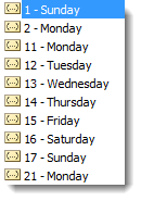
The full list of options for WEEKNUM is as follows:
Counting and Tracking Dates
Dates can be added and subtracted like normal numbers because they’re stored as serial numbers. That lets you count the days between two different dates. Sometimes, though, you need to count by a different metric.
NETWORKDAYS()
Above, we learned about WORKDAY, which lets you move back and forth a set number of workdays, ignoring weekends and holidays. But what if you need to measure the number of workdays between two dates? For that, Excel provides NETWORKDAYS. The formula syntax is as follows:
=NETWORKDAYS(start_date, end_date, [holidays])
The start_date and end_date can be any date-formatted cell reference.
The [holidays] input is optional, but lets you disqualify specific days (like Thanksgiving or Christmas, for example), which might otherwise fall during the work week. These are date serial numbers provided in an array bounded by brackets: { }. To specify multiple holidays, the dates must be held in cells – it is not possible to put multiple DATE functions in an array.
For example, if A1 contains 6:00pm (18:00 hours) on September 10, 2013 and B1 contains 9:00am (9:00 hours) on December 2, 2013, we can use NETWORKDAYS to find the number of workdays between the two dates.
Let’s exclude Columbus Day (October 14, 2013), Veterans Day (November 11, 2013), and Thanksgiving Day (November 28, 2013) as holidays. To do so, we have to store those dates in other cells. Let’s put them in C1, C2, and C3:
=DATE(2013,10,14)
=DATE(2013,11,11)
=DATE(2013,11,28)
Now, we can combine them in the function:
=NETWORKDAYS(A1,B1,C1:C3)
The function returns 57 as a numeric value.
NETWORKDAYS.INTL() (Excel 2010 and newer)
For newer versions of Excel (2010 and later), there is another version of NETWORKDAYS called NETWORKDAYS.INTL. NETWORKDAYS.INTL works just like NETWORKDAYS, but it adds the ability to customize the definition of the “weekend”. The syntax for NETWORKDAYS.INTL is as follows:
=NETWORKDAYS.INTL(start_date, end_date, [weekend], [holidays])
The start_date, end_date, and [holidays] inputs work just like the normal WORKDAY function.
The [weekend] input has the following options:
YEARFRAC()
Sometimes it’s useful to measure how much time has passed in years, but subtracting the YEAR function will only round down to the nearest full year. YEARFRAC takes two dates and provides the portion of the year between them. The syntax is as follows:
=YEARFRAC(start_date, end_date, [basis])
The start_date and end_date can be any date-formatted cell reference.
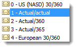
The [basis] input is optional, but lets you specify the “rules” for measuring the difference. Most of the time, you’ll want to use option 1, but here is the full list:
 For example, if A1 contains September 10, 2013 and B1 contains December 2, 2013, we can use YEARFRAC to find the decimal portion of a year between the two dates:
=YEARFRAC(A1,B1,1)
Returns 0.227397260273973.
DATEDIF() (Undocumented Function)
The YEARFRAC function gives you the difference between dates as a fraction of a year, but sometimes you need more control. There is a powerful hidden function in Excel called DATEDIF that can do much more. It can tell you the number of years, months, or days between two dates. It can also track based on only partial inputs, ignoring years or months when calculating days. The syntax for DATEDIF is as follows:
=DATEDIF(start_date, end_date, unit)
The start_date and end_date can be any date-formatted cell reference.
The unit input asks you to specify a string that represents the type of output you want. This is slightly cumbersome, since you must wrap the input in quotes (” “).
For example, if A1 contains September 10, 2012 and B1 contains December 2, 2013, we can use DATEDIF to find the number of full years between the two dates:
=DATEDIF(A1,B1,"Y")
Returns 1 as a numeric value.
Using the same start_date and end_date inputs, here are the output possibilities for DATEDIF using different unit parameters:
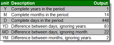
Every time, the unit must be put in quotes (e.g. “Y” or “MD”).
Converting Dates and Times from Text
DATEVALUE() and TIMEVALUE()
All of the above functions work perfectly with date-formatted serial numbers in Excel. Unfortunately, dates and times are often imported into worksheets as text. Most of the assorted functions like MONTH and HOUR are reasonably intelligent about converting on the fly. Occasionally it’s useful to build a date value through concatenation. The two functions Excel provides for this purpose are DATEVALUE and TIMEVALUE. The syntax for each is as follows:
=DATEVALUE(date_text)
=TIMEVALUE(time_text)
The date_text and time_text accept any text string that looks like a date or time.
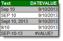
This is how DATEVALUE responds to various date_text inputs:
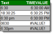
This is how TIMEVALUE responds to various time_text inputs:
Converting Dates and Times to Text
TEXT()
Getting data converted to dates and times is great, but you may also need to get it back out. Sometimes, you need a special format. Other times, you need to look for a date in a text string, and have to match using string tools like FIND and SEARCH. There is one master function for converting dates and times to text strings in Excel, called TEXT. The syntax for TEXT is as follows:
=TEXT(value, format_text)
The value can be any date or time-formatted cell reference.
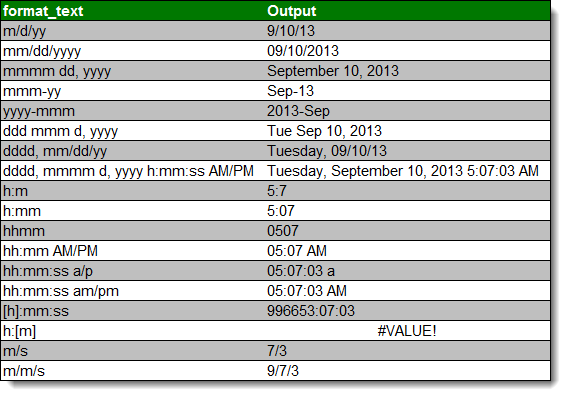
The format_text input has a large number of options, summarized here:
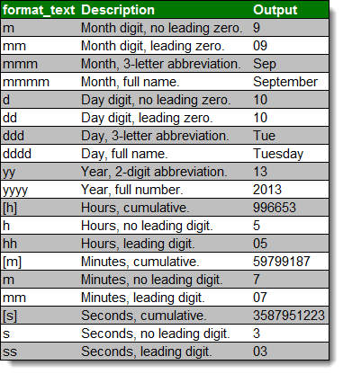
The outputs can be combined with simple formatting characters to produce standard date formats. Using the date 5:07:03am (05:07 hours, 3 seconds) on September 10, 2013, here are examples of possible outputs:
A Common Problem
One issue people frequently run into is that Excel occasionally misinterprets text fields as dates. An example is here:
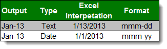
Be careful when entering dates, especially if you are importing from other data sources, to make sure that your “Jan-13” is being stored as January 1, 2013 and not January 13, 2013!
Get the latest Excel tips and tricks by joining the newsletter!
 Andrew Roberts has been solving business problems with Microsoft Excel for over a decade. Excel Tactics is dedicated to helping you master it.
Join the newsletter to stay on top of the latest articles. Sign up and you’ll get a free guide with 10 time-saving keyboard shortcuts!
Other posts in this series…
The easiest and fastest way to enter into the cell current date or time — is to click the hotkey combination CTRL + «;» (today’s date) and CTRL + SHIFT + «;» (the current time).
To use the TODAY () function is much better. It not only states but also automatically updates the information of the cell every day without user intervention.
How to put the current date in Excel
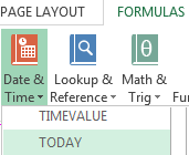
To insert the current date in Excel a person should use the function TODAY (). To do this, select the tool «FORMULAS»-«Date & Time»-«TODAY». This function has no arguments, so you can just type in a cell «=TODAY()» and press ENTER.
The current date in a cell:
If it is necessary to update automatically not only the current date, but the time in the cell, you’d better use the function «=NOW()».
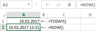
The current date and time in a cell.
The way to set the current date into the running title in Excel
Inserting the current date in Excel is implemented in several ways:
- By setting the parameters of the running title. The advantage of this method is that the current date and time are put on all the pages at once simultaneously.
- Using the function TODAY ().
- Using the hotkey combination CTRL +; — To set the current date and CTRL + SHIFT +; — To set the current time. The disadvantage in this process is that it will not be automatically updated to the current value of the cell parameters, the document is opened. But in some cases, lack of data is an advantage.
- With the help of VBA macros using the function code of the program: Date();Time();Now();.
The running title allows you to set the current date and time in the top or bottom of pages in the document to be output to the printer. In addition, the header allows us to enumerate all the pages of the document.
To make the current date in Excel and enumerate the pages with the help of the running page you should:
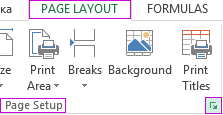
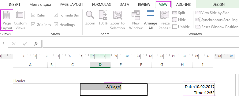
- Open the «PAGE LAYOUT»-«Page Setup» tab and select «Header/Footer».
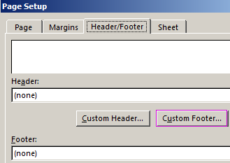
- Click on the button to create «Custom Footer».
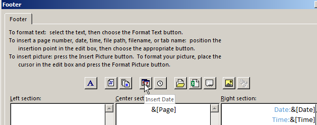
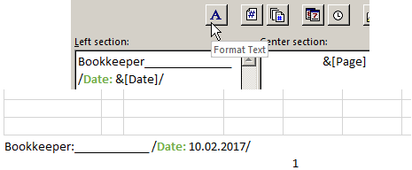
- In the window that appears, click on the field «Center section:». On the panel, click the second button, «Insert Number of Pages». Then select the first button «Format Text» and set the format to display the page number (for example, bold and font size of 14 points).
- To set the current date and time, click on the field «Right section:» and then click «Insert Date» (if necessary, click on the «Insert Time»). Click OK in both dialog boxes. In these fields you can enter your text.
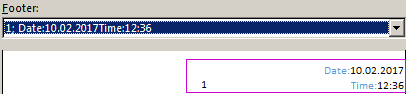
- Click OK, and look at the preliminary results display header. Below dropdown list «Footer:»
- «VIEW»-«Page Layout» menu, go to the preview of headers and footers. You can edit them there.
Running titles allow us not only to set the date and page number. You can also add a space for the signature of the responsible person for the report. For example, the edit is now the lower left part of the page in the running titles:
Thus, it is possible to create documents with a comfortable place for signatures and seals on each page automatically.
How to change date format in Excel 365 Online
Are you having a problem with date formatting in Excel 365 online? For example, are you finding your dates are showing as an American date format of mm/dd/yyyy or maybe the opposite with a UK date format of dd/mm/yyyy?
In this blog I’ll take you through a few things you can check in Excel 365 Desktop and Excel 365 Online so that you can change your date format to the Excel date format you require.
Why is the Excel 365 Online date format not working?
You may be experiencing problems within your own files, files you share with others, or both.
Saving files into OneDrive or SharePoint is a fantastic way for team members to be updating and working with files from outside of the office, and an excellent way for everyone to have access to the same file either inside or outside of the office.
However, it can be super frustrating when data is entered incorrectly as this impacts everyone using the file, and fixing formatting problems can be such a waste of your precious time.
Different date formats
Our client’s team had a problem with date formatting in Excel 365 Online when some members were updating dates in a shared file in the Desktop version of Excel 365, and others were updating dates in the same file using Excel 365 online, the web browser version.
Some team members were using both Excel 365 for Desktop when working in the office, and Excel 365 Online when working from home.
When dates were entered using Excel 365 desktop the date format was correct.
Sadly, the date formats kept changing when anyone accessing the file using Excel 365 online updated the file.
The team continually battled with dates entered as mm/dd/yyyy when they would normally use the dd/mm/yyyy format.
Additionally, some dates were aligned to the left of the cell and some to the right and this was happening in both the desktop and web versions of Excel.
This is how we fixed it.
Tip #1 Check the Date format in Excel Desktop
The first thing we checked was the date formatting had been set correctly as dd/mm/yyyy in Excel 365 Desktop.
We work with a New Zealand date format of day/month/year, a.k.a dd/mm/yyyy, e.g. 31/01/2022.
Change the date format in Excel Desktop
1. To check the current date format first select the cell range containing the dates, and then right-click any cell in the selected range.
2. Click Format Cells.
3. On the Number tab click Date and then check that your date is set to the format you require. You can see in the image below that ours is set to dd/mm/yyyy and the Sample box shows the date as 31/01/2022 which is exactly how we are wanting it to be displayed.
Also, check that the Locale option is set to your location. Ours is set correctly with English (New Zealand).
Notes: if the Date format is set incorrectly here you can select the format you require from the Date options.
Additionally, if the date format is showing as an American date format, you can easily change the date format in Excel by selecting Custom from the Category group, and then changing the Excel date format to the format you require.
You can see in the image below that ours is set to dd/mm/yyyy and the Sample box shows the date as 31/01/2022 which is exactly how we are wanting it to be displayed for our New Zealand date format.
If you wanted month/day/year you could enter a new format into the Type box. For example, for an American date format you could type mm/dd/yyyy, as shown below.
Excel Online date format not working
We found that the date settings were set correctly in Excel 365 Desktop.
However, even if we clicked OK to reapply the formatting on every selected cell, we still had several cells that were still formatted incorrectly with the date still left-aligned in the column.
We used the steps in Tip #3 below to reset the dates to the correct format.
Additionally, as soon as a team member accessed the file using Excel 365 Online the dates went back to being formatted incorrectly.
We then tried the steps in Tip #2.
Tip #2 Change the date format in Excel 365 Online
When team members were editing the sheet in the browser version of Excel (Excel 365 Online) the formatting changed to month/day/year, a.k.a mm/dd/yyyy, even though the date formats were set correctly in Excel 365 Desktop.
This was the reason some of the dates were being left-aligned in the column. For example, 31/01/2022 was being entered incorrectly because the web version of Excel 365 was seeing the date as mm/dd/yyyy. Since there isn’t a 31st month, Excel saw this as a mistype and entered the date as text, not a date.
However, because the date format was set to read month then day, entering 01/02/2022 was being entered as a date but it was being held as the 2nd of January, not the 1st of February.
Change the Date Format in Excel 365 Online
We followed the same steps as for Excel 365 Desktop to check the current Excel date format. To do this follows these steps.
1. Login to your Excel 365 Online account and open the file.
2. Select the cell range containing the dates, and then right-click any cell in the selected range.
3. Click Number Format.
4. On the Custom option we can see that the date format is set to dd/mm/yyyy. However, the dates were still being formatted incorrectly.
Note: there isn’t currently a way to change the date format within the Custom area in Excel 365 Online. To do this you will need to open the file into Excel 365 Desktop and follow the steps outlined above.
5. Click Date in the Category list.
6. Now, this is the important part. Check the Locale (location) setting. We had such a mix of settings for this. Some members of the team had English (United States), while others had Armenian or Azerbaijani!
7. Now select the correct date format you require from the Type list.
8. Select your location from the Locale (location) list.
Note: please be aware that changing the Regional format settings in Excel affect dates, currency, formula delimiters and more. For more information, please check the Microsoft support page online.
9. BEFORE you click OK be sure to select the Set this locate as the preferred regional format option box. If you don’t do this the date format will change itself back to its former setting again.
10. When you click OK the file will update.
11. Once the new date format is in place all dd/mm/yyyy date entries will be formatted with the correct Excel date format. If you find existing date entries still haven’t updated, please check the steps in Tip #3 below.
Note: you can also change the Excel 365 Online Regional format settings through File, Options. To do this follow the steps below.
1. Click the File tab and then click the 3 dots for access the More File Options.
2. Select Options.
3. Now click Regional Format Settings.
4. Select your preferred regional format from the drop-down list and then click Change.
Tip #3 Change existing dates to the correct date format in Excel
The tips above will set your date format for all dates entered going forward.
However, you may now be left with existing dates that are still in the incorrect format.
Let’s look at a quick way to fix this.
1. Select the cells that need to be reformatted with the correct date format.
2. From the Data tab select Text to Columns.
3. Follow the instruction for the version of Excel you are working in.
Change existing dates in Excel 365 Online
Remove the selection from all the Delimiter options and then click Apply.
Change existing dates in Excel 365 for Desktop
1. On Step 1 of the Convert Text to Columns Wizard select Delimited and then click Next.
2. On Step 2, leave all the delimiter options unchecked and then click Next.
3. On Step 3, select Date from the Column data format option box, and then select the format that the date is currently using. For example, if your date format is currently mm/dd/yy, and you want to change it to your default locale setting, select MDY. If it is dd/mm/yy and you want the dates to be formatted as American date format select DMY.
4. Click Finish.
Your dates will now be updated and the correct Date Formats reapplied.
Was this blog helpful? Let us know in the Comments below.
Instructions
Change the date format in Excel Desktop
- Select the cell range containing the dates, and then right-click any cell in the selected range.
- Click Format Cells.
- On the Number tab click Date and then check that your date is set to the format you require. Also, check that the Locale option is set to your location.
Change the Date Format in Excel 365 Online
- Login to your Excel 365 Online account and open the file.
- Select the cell range containing the dates, and then right-click any cell in the selected range.
- Click Number Format.
- On the Custom option we can see that the date format is set to dd/mm/yyyy.
- Click Date in the Category list.
- Check the Locale (location) setting.
- Now select the correct date format you require from the Type list.
- Select your location from the Locale (location) list.
- BEFORE you click OK be sure to select the Set this locate as the preferred regional format option box. If you don’t do this the date format will change itself back to its former setting again.
- When you click OK the file will update.
Change existing dates to the correct date format in Excel
The tips above will set your date format for all dates entered going forward. However, you may now be left with existing dates that are still in the incorrect format. To fix this:
- Select the cells that need to be reformatted with the correct date format.
- From the Data tab select Text to Columns.
- Follow the instruction for the version of Excel you are working in.
Change existing dates in Excel 365 Online
Remove the selection from all the Delimiter options and then click Apply.
Change existing dates in Excel 365 for Desktop
- On Step 1 of the Convert Text to Columns Wizard select Delimited and then click Next.
- On Step 2, leave all the delimiter options unchecked and then click Next.
- On Step 3, select Date from the Column data format option box, and then select the format that the date is currently using. For example, if your date format is currently mm/dd/yy, and you want to change it to your default locale setting, select MDY. If it is dd/mm/yy and you want the dates to be formatted as American date format select DMY.
- Click Finish.
Notes
Why is the Excel 365 Online date format not working?
Different date formats: Our client’s team had a problem with date formatting in Excel 365 Online when some members were updating dates in a shared file in the Desktop version of Excel 365, and others were updating dates in the same file using Excel 365 online, the web browser version. The team continually battled with dates entered as mm/dd/yyyy when they would normally use the dd/mm/yyyy format.
Change the date format in Excel Desktop
Note: if the Date format is set incorrectly in the Format Cells display box you can select the format you require from the Date options. Additionally, if the date format is showing as an American date format, you can easily change the date format in Excel by selecting Custom from the Category group, and then changing the Excel date format to the format you require. If you wanted month/day/year you could enter a new format into the Type box. For example, for an American date format you could type mm/dd/yyyy.
Change the Date Format in Excel 365 Online
Note: there isn’t currently a way to change the date format within the Custom area in Excel 365 Online.
Note: please be aware that changing the Regional format settings in Excel affect dates, currency, formula delimiters and more.
Change the Excel 365 Online Regional Format settings
- Click the File tab and then click the 3 dots for access the More File Options.
- Select Options.
- Now click Regional Format Settings.
- Select your preferred regional format from the drop-down list and then click Change.
Elevate your Excel game and become a pro with our exclusive Insider Group.
Be the first to know about new tutorials, videos, and tips for Microsoft 365 products. Join us now and claim your exclusive bonus today!