Excel for Microsoft 365 Excel for Microsoft 365 for Mac Excel for the web Excel 2021 Excel 2021 for Mac Excel 2019 Excel 2019 for Mac Excel 2016 Excel 2016 for Mac Excel 2013 Excel 2010 Excel 2007 Excel for Mac 2011 Excel Starter 2010 More…Less
Use Excel’s DATE function when you need to take three separate values and combine them to form a date.
The DATE function returns the sequential serial number that represents a particular date.
Syntax: DATE(year,month,day)
The DATE function syntax has the following arguments:
-
Year Required. The value of the year argument can include one to four digits. Excel interprets the year argument according to the date system your computer is using. By default, Microsoft Excel for Windows uses the 1900 date system, which means the first date is January 1, 1900.
Tip: Use four digits for the year argument to prevent unwanted results. For example, «07» could mean «1907» or «2007.» Four digit years prevent confusion.
-
If year is between 0 (zero) and 1899 (inclusive), Excel adds that value to 1900 to calculate the year. For example, DATE(108,1,2) returns January 2, 2008 (1900+108).
-
If year is between 1900 and 9999 (inclusive), Excel uses that value as the year. For example, DATE(2008,1,2) returns January 2, 2008.
-
If year is less than 0 or is 10000 or greater, Excel returns the #NUM! error value.
-
-
Month Required. A positive or negative integer representing the month of the year from 1 to 12 (January to December).
-
If month is greater than 12, month adds that number of months to the first month in the year specified. For example, DATE(2008,14,2) returns the serial number representing February 2, 2009.
-
If month is less than 1, month subtracts the magnitude of that number of months, plus 1, from the first month in the year specified. For example, DATE(2008,-3,2) returns the serial number representing September 2, 2007.
-
-
Day Required. A positive or negative integer representing the day of the month from 1 to 31.
-
If day is greater than the number of days in the month specified, day adds that number of days to the first day in the month. For example, DATE(2008,1,35) returns the serial number representing February 4, 2008.
-
If day is less than 1, day subtracts the magnitude that number of days, plus one, from the first day of the month specified. For example, DATE(2008,1,-15) returns the serial number representing December 16, 2007.
-
Note: Excel stores dates as sequential serial numbers so that they can be used in calculations. January 1, 1900 is serial number 1, and January 1, 2008 is serial number 39448 because it is 39,447 days after January 1, 1900. You will need to change the number format (Format Cells) in order to display a proper date.
Syntax: DATE(year,month,day)
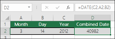
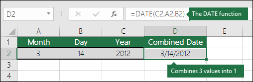
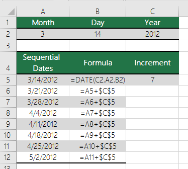
For example: =DATE(C2,A2,B2) combines the year from cell C2, the month from cell A2, and the day from cell B2 and puts them into one cell as a date. The example below shows the final result in cell D2.
Need to insert dates without a formula? No problem. You can insert the current date and time in a cell, or you can insert a date that gets updated. You can also fill data automatically in worksheet cells.
-
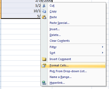
Right-click the cell(s) you want to change. On a Mac, Ctrl-click the cells.
-
On the Home tab click Format > Format Cells or press Ctrl+1 (Command+1 on a Mac).
-
3. Choose the Locale (location) and Date format you want.
-
For more information on formatting dates, see Format a date the way you want.

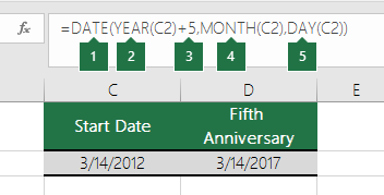
You can use the DATE function to create a date that is based on another cell’s date. For example, you can use the YEAR, MONTH, and DAY functions to create an anniversary date that’s based on another cell. Let’s say an employee’s first day at work is 10/1/2016; the DATE function can be used to establish his fifth year anniversary date:
-
The DATE function creates a date.
=DATE(YEAR(C2)+5,MONTH(C2),DAY(C2))
-
The YEAR function looks at cell C2 and extracts «2012».
-
Then, «+5» adds 5 years, and establishes «2017» as the anniversary year in cell D2.
-
The MONTH function extracts the «3» from C2. This establishes «3» as the month in cell D2.
-
The DAY function extracts «14» from C2. This establishes «14» as the day in cell D2.
If you open a file that came from another program, Excel will try to recognize dates within the data. But sometimes the dates aren’t recognizable. This is may be because the numbers don’t resemble a typical date, or because the data is formatted as text. If this is the case, you can use the DATE function to convert the information into dates. For example, in the following illustration, cell C2 contains a date that is in the format: YYYYMMDD. It is also formatted as text. To convert it into a date, the DATE function was used in conjunction with the LEFT, MID, and RIGHT functions.

-
The DATE function creates a date.
=DATE(LEFT(C2,4),MID(C2,5,2),RIGHT(C2,2))
-
The LEFT function looks at cell C2 and takes the first 4 characters from the left. This establishes “2014” as the year of the converted date in cell D2.
-
The MID function looks at cell C2. It starts at the 5th character, and then takes 2 characters to the right. This establishes “03” as the month of the converted date in cell D2. Because the formatting of D2 set to Date, the “0” isn’t included in the final result.
-
The RIGHT function looks at cell C2 and takes the first 2 characters starting from the very right and moving left. This establishes “14” as the day of the date in D2.
To increase or decrease a date by a certain number of days, simply add or subtract the number of days to the value or cell reference containing the date.
In the example below, cell A5 contains the date that we want to increase and decrease by 7 days (the value in C5).
See Also
Add or subtract dates
Insert the current date and time in a cell
Fill data automatically in worksheet cells
YEAR function
MONTH function
DAY function
TODAY function
DATEVALUE function
Date and time functions (reference)
All Excel functions (by category)
All Excel functions (alphabetical)
Need more help?
Содержание
- DATE function
- How to conditionally format dates and time in Excel with formulas and inbuilt rules
- Excel conditional formatting for dates (built-in rules)
- Excel conditional formatting formulas for dates
- How to highlight weekends in Excel
- How to highlight holidays in Excel
- Conditionally format a cell when a value is changed to a date
- How to highlight rows based on a certain date in a certain column
- Conditionally format dates in Excel based on the current date
- Example 1. Highlight dates equal to, greater than or less than today
- Example 2. Conditionally format dates in Excel based on several conditions
- Example 3. Highlight upcoming dates and delays
- How to highlight dates within a date range
- How to shade gaps and time intervals
- «Days Until Next Birthday» Excel Web App
DATE function
Use Excel’s DATE function when you need to take three separate values and combine them to form a date.
The DATE function returns the sequential serial number that represents a particular date.
The DATE function syntax has the following arguments:
Year Required. The value of the year argument can include one to four digits. Excel interprets the year argument according to the date system your computer is using. By default, Microsoft Excel for Windows uses the 1900 date system, which means the first date is January 1, 1900.
Tip: Use four digits for the year argument to prevent unwanted results. For example, «07» could mean «1907» or «2007.» Four digit years prevent confusion.
If year is between 0 (zero) and 1899 (inclusive), Excel adds that value to 1900 to calculate the year. For example, DATE(108,1,2) returns January 2, 2008 (1900+108).
If year is between 1900 and 9999 (inclusive), Excel uses that value as the year. For example, DATE(2008,1,2) returns January 2, 2008.
If year is less than 0 or is 10000 or greater, Excel returns the #NUM! error value.
Month Required. A positive or negative integer representing the month of the year from 1 to 12 (January to December).
If month is greater than 12, month adds that number of months to the first month in the year specified. For example, DATE(2008,14,2) returns the serial number representing February 2, 2009.
If month is less than 1, month subtracts the magnitude of that number of months, plus 1, from the first month in the year specified. For example, DATE(2008,-3,2) returns the serial number representing September 2, 2007.
Day Required. A positive or negative integer representing the day of the month from 1 to 31.
If day is greater than the number of days in the month specified, day adds that number of days to the first day in the month. For example, DATE(2008,1,35) returns the serial number representing February 4, 2008.
If day is less than 1, day subtracts the magnitude that number of days, plus one, from the first day of the month specified. For example, DATE(2008,1,-15) returns the serial number representing December 16, 2007.
Note: Excel stores dates as sequential serial numbers so that they can be used in calculations. January 1, 1900 is serial number 1, and January 1, 2008 is serial number 39448 because it is 39,447 days after January 1, 1900. You will need to change the number format (Format Cells) in order to display a proper date.
For example: =DATE(C2,A2,B2) combines the year from cell C2, the month from cell A2, and the day from cell B2 and puts them into one cell as a date. The example below shows the final result in cell D2.
Need to insert dates without a formula? No problem. You can insert the current date and time in a cell, or you can insert a date that gets updated. You can also fill data automatically in worksheet cells.
Right-click the cell(s) you want to change. On a Mac, Ctrl-click the cells.
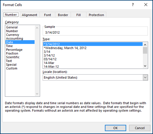
On the Home tab click Format > Format Cells or press Ctrl+1 (Command+1 on a Mac).
3. Choose the Locale (location) and Date format you want.
For more information on formatting dates, see Format a date the way you want.
You can use the DATE function to create a date that is based on another cell’s date. For example, you can use the YEAR, MONTH, and DAY functions to create an anniversary date that’s based on another cell. Let’s say an employee’s first day at work is 10/1/2016; the DATE function can be used to establish his fifth year anniversary date:
The DATE function creates a date.
The YEAR function looks at cell C2 and extracts «2012».
Then, «+5» adds 5 years, and establishes «2017» as the anniversary year in cell D2.
The MONTH function extracts the «3» from C2. This establishes «3» as the month in cell D2.
The DAY function extracts «14» from C2. This establishes «14» as the day in cell D2.
If you open a file that came from another program, Excel will try to recognize dates within the data. But sometimes the dates aren’t recognizable. This is may be because the numbers don’t resemble a typical date, or because the data is formatted as text. If this is the case, you can use the DATE function to convert the information into dates. For example, in the following illustration, cell C2 contains a date that is in the format: YYYYMMDD. It is also formatted as text. To convert it into a date, the DATE function was used in conjunction with the LEFT, MID, and RIGHT functions.
The DATE function creates a date.
The LEFT function looks at cell C2 and takes the first 4 characters from the left. This establishes “2014” as the year of the converted date in cell D2.
The MID function looks at cell C2. It starts at the 5th character, and then takes 2 characters to the right. This establishes “03” as the month of the converted date in cell D2. Because the formatting of D2 set to Date, the “0” isn’t included in the final result.
The RIGHT function looks at cell C2 and takes the first 2 characters starting from the very right and moving left. This establishes “14” as the day of the date in D2.
To increase or decrease a date by a certain number of days, simply add or subtract the number of days to the value or cell reference containing the date.
In the example below, cell A5 contains the date that we want to increase and decrease by 7 days (the value in C5).
Источник
How to conditionally format dates and time in Excel with formulas and inbuilt rules
 by Svetlana Cheusheva, updated on February 7, 2023
If you are a regular visitor of this blog, you’ve probably noticed a few articles covering different aspects of Excel conditional formatting. And now we will leverage this knowledge and create spreadsheets that differentiate between weekdays and weekends, highlight public holidays and display a coming deadline or delay. In other words, we are going to apply Excel conditional formatting to dates.
If you have some basic knowledge of Excel formulas, then you are most likely familiar with some of date and time functions such as NOW, TODAY, DATE, WEEKDAY, etc. In this tutorial, we are going to take this functionality a step further to conditionally format Excel dates in the way you want.
Excel conditional formatting for dates (built-in rules)
Microsoft Excel provides 10 options to format selected cells based on the current date.
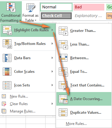
- To apply the formatting, you simply go to the Home tab >Conditional Formatting > Highlight Cell Rules and select A Date Occurring.
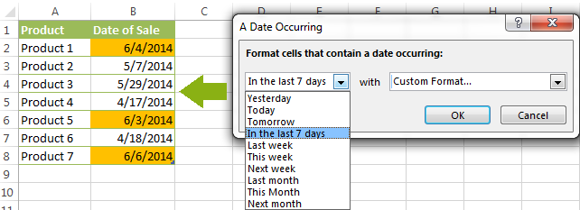
- Select one of the date options from the drop-down list in the left-hand part of the window, ranging from last month to next month.
- Finally, choose one of the pre-defined formats or set up your custom format by choosing different options on the Font, Border and Fill tabs. If the Excel standard palette does not suffice, you can always click the More colors… button.
- Click OK and enjoy the result! : )

However, this fast and straightforward way has two significant limitations — 1) it works for selected cells only and 2) the conditional format is always applied based on the current date.
Excel conditional formatting formulas for dates
If you want to highlight cells or entire rows based on a date in another cell, or create rules for greater time intervals (i.e. more than a month from the current date), you will have to create your own conditional formatting rule based on a formula. Below you will find a few examples of my favorite Excel conditional formats for dates.
How to highlight weekends in Excel
Regrettably, Microsoft Excel does not have a built-in calendar similar to Outlook’s. Well, let’s see how you can create your own automated calendar with quite little effort.
When designing your Excel calendar, you can use the =DATE(year,month,date) function to display the days of the week. Simply enter the year and the month’s number somewhere in your spreadsheet and reference those cells in the formula. Of course, you could type the numbers directly in the formula, but this is not a very efficient approach because you would have to adjust the formula for each month.
The screenshot below demonstrates the DATE function in action. I used the formula =DATE($B$2,$B$1,B$4) which is copied across row 5. 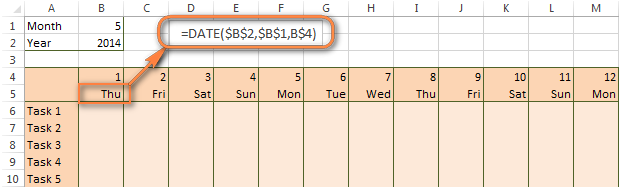
Tip. If you want to display only the days of the week like you see in the image above, select the cells with the formula (row 5 in our case), right-click and choose Format Cells…> Number > Custom. From the drop-down list under Type, select either dddd or ddd to show full day names or abbreviated names, respectively.
Your Excel calendar is almost done, and you only need to change the color of weekends. Naturally, you are not going to color the cells manually. We’ll have Excel format the weekends automatically by creating a conditional formatting rule based on the WEEKDAY formula.
- You start by selecting your Excel calendar where you want to shade the weekends. In our case, it is the range $B$4:$AE$10. Be sure to start the selection with the 1 st date column — Colum B in this example.
- On the Home tab, click Conditional Formatting menu > New Rule.
- Create a new conditional formatting rule based on a formula as explained in the above linked guide.
- In the «Format values where this formula is true» box, enter the following WEEKDAY formula that will determine which cells are Saturdays and Sundays: =WEEKDAY(B$5,2)>5
- Click the Format… button and set up your custom format by switching between the Font, Border and Fill tabs and playing with different formatting options. When done, click the OK button to preview the rule.

Now, let me briefly explain the WEEKDAY(serial_number,[return_type]) formula so that you can quickly adjust it for your own spreadsheets.
- The serial_number parameter represents the date you are trying to find. You enter a reference to your first cell with a date, B$5 in our case.
- The [return_type] parameter determines the week type (square brackets imply it is optional). You enter 2 as the return type for a week starting from Monday (1) through Sunday (7). You can find the full list of available return types here.
- Finally, you write >5 to highlight only Saturdays (6) and Sundays (7).
The screenshot below demonstrates the result in Excel 2013 — the weekends are highlighted in the reddish colour. 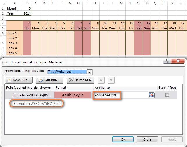
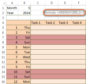
- If you have non-standard weekends in your company, e.g. Fridays and Saturdays, then you would need to tweak the formula so that it starts counting from Sunday (1) and highlight days 6 (Friday) and 7 (Saturday) — WEEKDAY(B$5,1)>5 .
- If you are creating a horizontal (landscape) calendar, use a relative column (without $) and absolute row (with $) in a cell reference because you should lock the reference of the row — in the above example it is row 5, so we entered B$5. But if you are designing a calendar in vertical orientation, you should do the opposite, i.e. use an absolute column and relative row, e.g. $B5 as you can see in the screenshot below:
How to highlight holidays in Excel
To improve your Excel calendar further, you can shade public holidays as well. To do that, you will need to list the holidays you want to highlight in the same or some other spreadsheet.
For example, I’ve added the following holidays in column A ($A$14:$A$17). Of course, not all of them are real public holidays, but they will do for demonstration purposes : ) 
Again, you open Conditional Formatting > New Rule. In the case of holidays, you are going to use either MATCH or COUNTIF function:
Note. If you have chosen a different color for holidays, you need to move the public holiday rule to the top of the rules list via Conditional Formatting > Manage Rules…
The following image shows the result in Excel 2013: 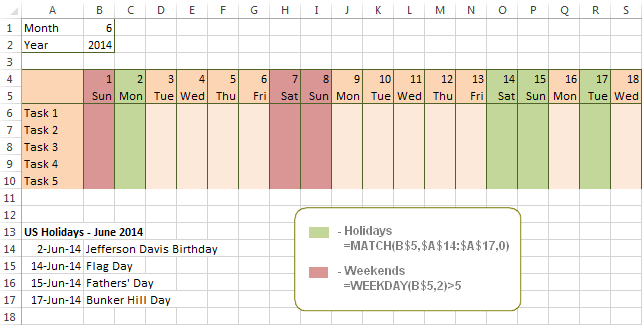
Conditionally format a cell when a value is changed to a date
It’s not a big problem to conditionally format a cell when a date is added to that cell or any other cell in the same row as long as no other value type is allowed. In this case, you could simply use a formula to highlight non-blanks, as described in Excel conditional formulas for blanks and non-blanks. But what if those cells already have some values, e.g. text, and you want to change the background color when text is changed to a date?
The task may sound a bit intricate, but the solution is very simple.
- First off, you need to determine the format code of your date. Here are just a few examples:
- D1: dd-mmm-yy or d-mmm-yy
- D2: dd-mmm or d-mmm
- D3: mmm-yy
- D4: mm/dd/yy or m/d/yy or m/d/yy h:mm
You can find the complete list of date codes in this article.
If your table contains dates in 2 or more formats, then use the OR operator, e.g. =OR(cell(«format», $A2)=»D1″, cell(«format»,$A2)=»D2″, cell(«format», $A2)=»D3″)
The screenshot below demonstrates the result of such conditional formatting rule for dates. 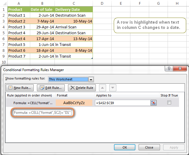
How to highlight rows based on a certain date in a certain column
Suppose, you have a large Excel spreadsheet that contains two date columns (B and C). You want to highlight every row that has a certain date, say 13-May-14, in column C.
To apply Excel conditional formatting to a certain date, you need to find its numerical value first. As you probably know, Microsoft Excel stores dates as sequential serial numbers, starting from January 1, 1900. So, 1-Jan-1900 is stored as 1, 2-Jan-1900 is stored as 2… and 13-May-14 as 41772.
To find the date’s number, right-click the cell, select Format Cells > Number and choose the General format. Write down the number you see and click Cancel because you do not really want to change the date’s format. 
That was actually the major part of the work and now you only need to create a conditional formatting rule for the entire table with this very simple formula: =$C2=41772 . The formula implies that your table has headers and row 2 is your first row with data.
An alternative way is to use the DATEVALUE formula that converts the date to the number format is which it is stored, e.g. =$C2=DATEVALUE(«5/13/2014»)
Whichever formula you use, it will have the same effect: 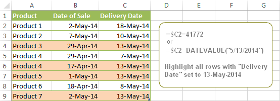
Conditionally format dates in Excel based on the current date
As you probably know Microsoft Excel provides the TODAY() functions for various calculations based on the current date. Here are just a few examples of how you can use it to conditionally format dates in Excel.
Example 1. Highlight dates equal to, greater than or less than today
To conditionally format cells or entire rows based on today’s date, you use the TODAY function as follows:
Equal to today: =$B2=TODAY()
Greater than today: =$B2>TODAY()
Less than today: =$B2
The screenshot below demonstrates the above rules in action. Please note, at the moment of writing TODAY was 12-Jun-2014. 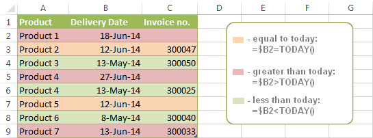
Example 2. Conditionally format dates in Excel based on several conditions
In a similar fashion, you can use the TODAY function in combination with other Excel functions to handle more complex scenarios. For example, you may want your Excel conditional formatting date formula to color the Invoice column when the Delivery Date is equal to or greater than today BUT you want the formatting to disappear when you enter the invoice number.
For this task, you would need an additional column with the following formula (where E is your Delivery column and F the Invoice column):
If the delivery date is greater than or equal to the current date and there is no number in the Invoice column, the formula returns 1, otherwise it’s 0.
After that you create a simple conditional formatting rule for the Invoice column with the formula =$G2=1 where G is your additional column. Of course, you will be able to hide this column later. 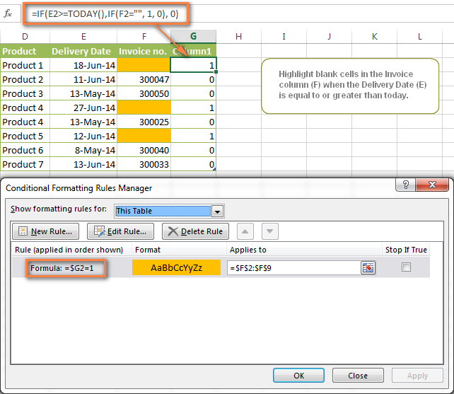
Example 3. Highlight upcoming dates and delays
Suppose you have a project schedule in Excel that lists tasks, their start dates and durations. What you want is to have the end date for each task calculated automatically. An additional challenge is that the formula should also consider the weekends. For example, if the starting date is 13-Jun-2014 and the number of days of work (Duration) is 2, the ending date should come as 17-Jun-2014, because 14-Jun and 15-Jun are Saturday and Sunday.
To do this, we will use the WORKDAY.INTL(start_date,days,[weekend],[holidays]) function, more precisely =WORKDAY.INTL(B2,C2,1) . 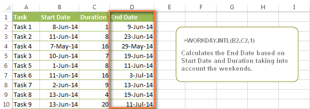
In the formula, we enter 1 as the 3 rd parameter since it indicates Saturday and Sunday as holidays. You can use another value if your weekends are different, say, Fri and Sat. The full list of the weekend values is available here. Optionally, you can also use the 4th parameter [holidays], which is a set of dates (range of cells) that should be excluded from the working day calendar.
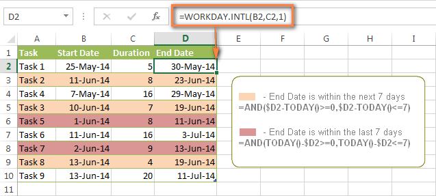
And finally, you may want to highlight rows depending on how far away the deadline is. For example, the conditional formatting rules based on the following 2 formulas highlight upcoming and recent end dates, respectively:
- =AND($D2-TODAY()>=0,$D2-TODAY() — highlight all rows where the End Date (column D) is within the next 7 days. This formula is really handy when it comes to tracking upcoming expiration dates or payments.
- =AND(TODAY()-$D2>=0,TODAY()-$D2 — highlight all rows where the End Date (column D) is within the last 7 days. You can use this formula to track the latest overdue payments and other delays.
Here are a few more formula examples that can be applied to the table above:
=$D2 — highlights all passed dates (i.e. dates less than the current date). Can be used to format expired subscriptions, overdue payments etc.
=$D2>TODAY() — highlights all future dates (i.e. dates greater than the current date). You can use it to highlight upcoming events.
Of course, there can be infinite variations of the above formulas, depending on your particular task. For instance:
=$D2-TODAY()>=6 — highlights dates that occur in 6 or more days.
=$D2=TODAY()-14 — highlights dates occurring exactly 2 weeks ago.
How to highlight dates within a date range
If you have a long list of dates in your worksheet, you may also want to highlight the cells or rows that fall within a certain date range, i.e. highlight all dates that are between two given dates.
You can fulfil this task using the TODAY() function again. You will just have to construct a little bit more elaborate formulas as demonstrated in the examples below.
Formulas to highlight past dates
- More than 30 days ago: =TODAY()-$A2>30
- From 30 to 15 days ago, inclusive: =AND(TODAY()-$A2>=15, TODAY()-$A2
- Less than 15 days ago: =AND(TODAY()-$A2>=1, TODAY()-$A2
The current date and any future dates are not colored. 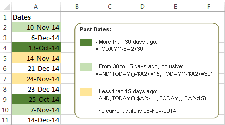
Formulas to highlight future dates
- Will occur in more than 30 days from now: =$A2-TODAY()>30
- In 30 to 15 days, inclusive: =AND($A2-TODAY()>=15, $A2-TODAY()
- In less than 15 days: =AND($A2-TODAY()>=1, $A2-TODAY()
The current date and any past dates are not colored. 
How to shade gaps and time intervals
In this last example, we are going to utilize yet another Excel date function — DATEDIF(start_date, end_date, interval) . This function calculates the difference between two dates based on the specified interval. It differs from all other functions we’ve discussed in this tutorial in the way that it lets you ignore months or years and calculate the difference only between days or months, whichever you choose.
Don’t see how this could work for you? Think about it in another way… Suppose you have a list of birthdays of your family members and friends. Would you like to know how many days there are until their next birthday? Moreover, how many days exactly are left until your wedding anniversary and other events you wouldn’t want to miss? Easily!
The formula you need is this (where A is your Date column):
=DATEDIF(TODAY(), DATE((YEAR(TODAY())+1), MONTH($A2), DAY($A2)), «yd»)
The «yd» interval type at the end of the formula is used to ignore years and calculate the difference between the days only. For the full list of available interval types, look here.
Tip. If you happen to forget or misplace that complex formula, you can use this simple one instead: =365-DATEDIF($A2,TODAY(),»yd») . It produces exactly the same results, just remember to replace 365 with 366 in leap years : )
And now let’s create an Excel conditional formatting rule to shade different gaps in different colors. In this case, it makes more sense to utilize Excel Color Scales rather than create a separate rule for each period.
The screenshot below demonstrates the result in Excel — a gradient 3-color scale with tints from green to red through yellow. 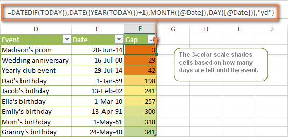
«Days Until Next Birthday» Excel Web App
We have created this Excel Web App to show you the above formula in action. Just enter your events in 1st column and change the corresponding dates in the 2nd column to experiment with the result.
Note. To view the embedded workbook, please allow marketing cookies.
If you are curious to know how to create such interactive Excel spreadsheets, check out this article on how to make web-based Excel spreadsheets.
Hopefully, at least one of the Excel conditional formats for dates discussed in this article has proven useful to you. If you are looking for a solution to some different task, you are most welcome to post a comment. Thank you for reading!
Источник
На чтение 5 мин Просмотров 4.3к. Опубликовано 19.02.2022
Excel сохраняет даты в виде порядковых номеров. Человеку невозможно их читать и понимать, но, таким образом, можно использовать их в функциях расчета, к примеру добавить к дате или времени какое-то количество времени (день, год и так далее).
Но, довольно часто, вам может быть нужно использовать даты в одних ячейках с текстом, так сказать, объединять.
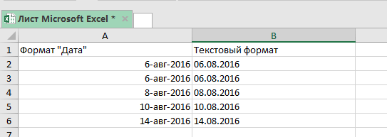
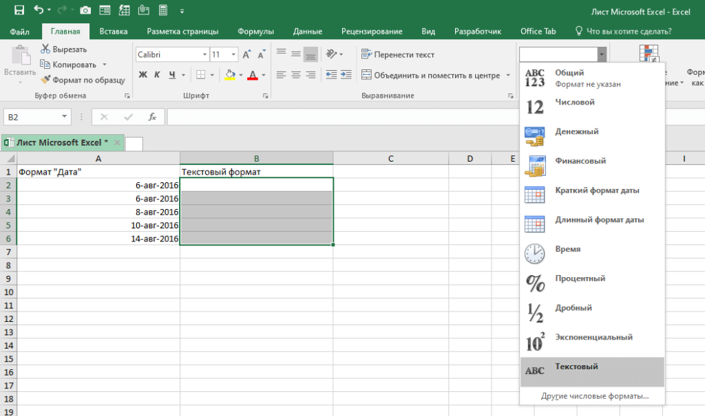
На картинке пример объединения даты с текстом в одной ячейке. Видите как выглядит наша дата? Это формат порядкового номера Excel.

Именно в таких ситуациях вам может понадобиться привести дату в «читаемый» формат.
Содержание
- Переводим дату в текстовый формат
- Как привести указанную дату в текстовый формат
- Как привести текущую дату в текстовый формат
- Переводим дату в текстовый формат с помощью функции «Текст по столбцам»
- Переводим дату в текстовый формат с помощью копирования и вставки
Переводим дату в текстовый формат
Когда нам нужно привести дату в определенный формат (к примеру, 16-08-2016), мы можем вызвать функцию ТЕКСТ.
Итак, как она работает.

Синтаксис:
=ТЕКСТ(значение; формат_текста)Она принимает два аргумента:
- Значение — в нашем случае это дата, которую вы хотите преобразовать в текст нужного формата. Это может быть просто дата, ссылка на ячейку с датой, или результат формулы.
- Формат_текста — формат, в котором нужно показать нашу дату. Формат должен быть указан в двойных кавычках.
Какие есть форматы и разделители?
Формат дат состоит из 4 составляющих:
- день
- месяц
- год
- разделитель
Ниже приведены форматы, которые можно использовать для каждой части:
Формат дня:
- Д — день будет отображаться без нуля, т.е. 1 будет отображаться как 1, а 12 как 12.
- ДД — день будет отображаться с нулем, т.е. 1 будет 01, а 12 как 12.
- ДДД — будет отображаться день недели(сокращенно), т.е. «Пятница» будет «Пят».
- ДДДД — будет отображаться день недели(полностью), т.е. «Пятница» будет «Пятница».
Формат месяца:
- М — месяц будет отображаться без нуля, т.е. 1 будет отображаться как 1, а 12 как 12.
- ММ — месяц будет отображаться с нулем, т.е. 1 будет 01, а 12 как 12.
- МММ — месяц будет отображаться с сокращенным названием, т.е. «Сентябрь» будет «Сен».
М — месяц будет отображаться без нуля, т.е. 1 будет отображаться как 1, а 12 как 12.
ММ — месяц будет отображаться с нулем, т.е. 1 будет 01, а 12 как 12.
МММ — месяц будет отображаться с сокращенным названием, т.е. «Сентябрь» будет «Сен».
ММММ — месяц будет отображаться с полным названием, т.е. «Сентябрь» будет «Сентябрь».
Формат года:
- ГГ — год будет отображаться как 2 цифры, т.е. 2019 будет 19.
- ГГГГ — год будет отображаться полностью, т.е. 2019 будет 2019.
Разделитель:
- «/» : это просто разделитель между цифрами в дате, т.е. отображаться будет как 01/01/2019.
- «-»: такой же разделитель между цифрами, т.е. отображаться будет как 01-01-2019.
- Пробелы и запятые: тут немного посложней, вы можете комбинировать и создавать свои форматы отображения, например, 01 января, 2019 года.
Итак, разберем примеры.
Как привести указанную дату в текстовый формат
Пример:
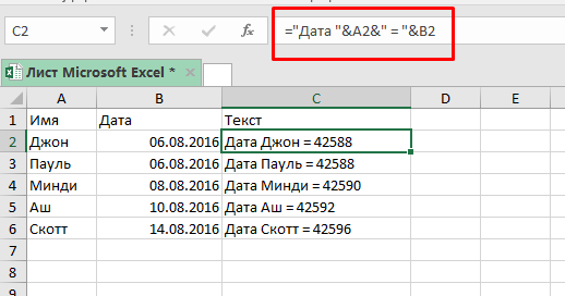
Итак, мы получили дату вместе с текстом, но дата сейчас в формате порядкового номера Excel.
Формула:
="Дата"&A2&"="&B2 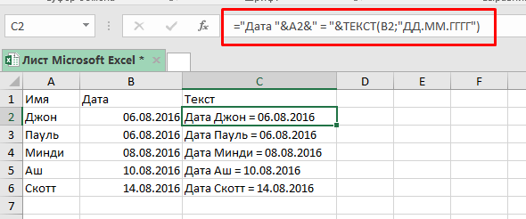
Теперь, нам нужно получить дату в «привычном» для нас виде.
Формула будет:
="Дата "&A2&" = "&ТЕКСТ(B2;"ДД.ММ.ГГГГ")Итак, мы вызвали функцию ТЕКСТ, указали ссылку на ячейку и определили формат, результат вы видите на картинке выше.
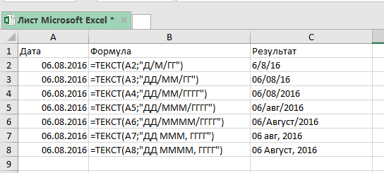
Какие еще есть форматы и как они выглядят на «выходе»:
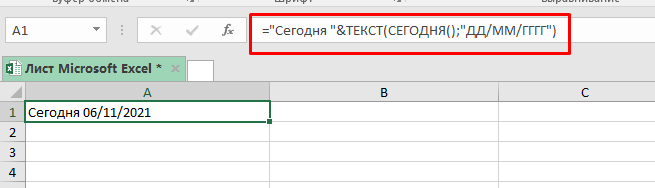
Как привести текущую дату в текстовый формат
Для того чтобы получить текущую дату мы можем использовать функцию СЕГОДНЯ.
Формула:
="Сегодня "&ТЕКСТ(СЕГОДНЯ();"ДД/ММ/ГГГГ")Эта функция может пригодиться вам в случае, если вы формируете отчеты, где важна, например, дата изменения файла.
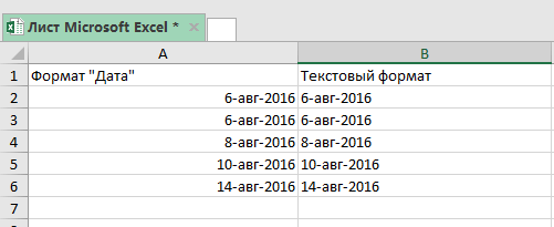
Переводим дату в текстовый формат с помощью функции «Текст по столбцам»
Если формулы и вызов функций вам не по душе, есть вариант и для вас.
Допустим, у нас есть следующие данные и нам нужно преобразовать их в текстовый формат:
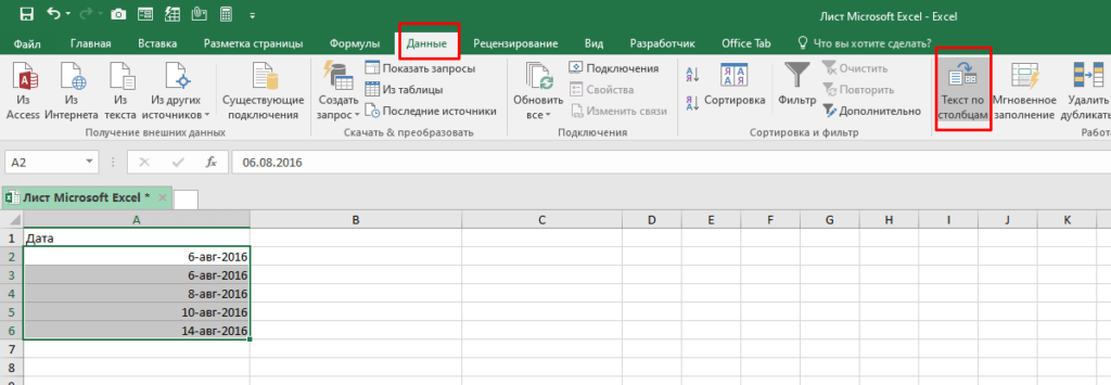
Пошаговая инструкция:
- Выделите ячейки, которые необходимо преобразовать в текст;
- Перейдите в раздел «Данные» -> «Текст по столбцам»;
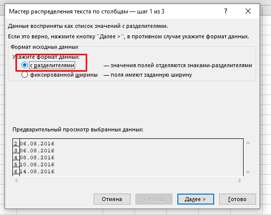
- В открывшемся окне:
- Выберите опцию «с разделителями»;
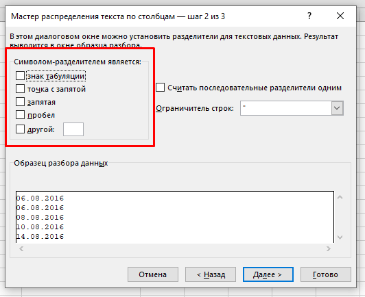
- Снимите все галочки и нажмите «Далее»;
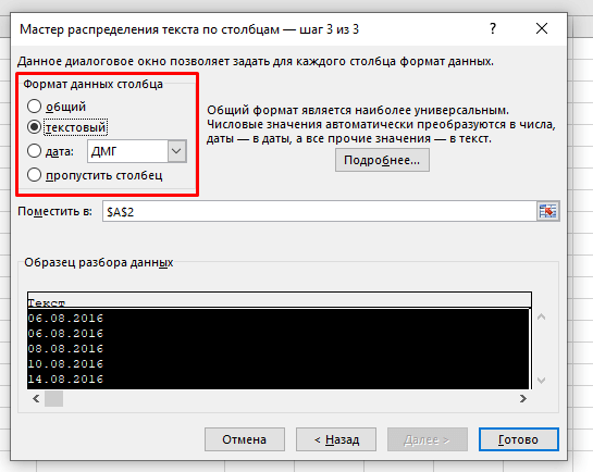
- Выберите формат «текстовый» укажите куда поместить наши, уже текстовые, значения и нажмите «Готово».
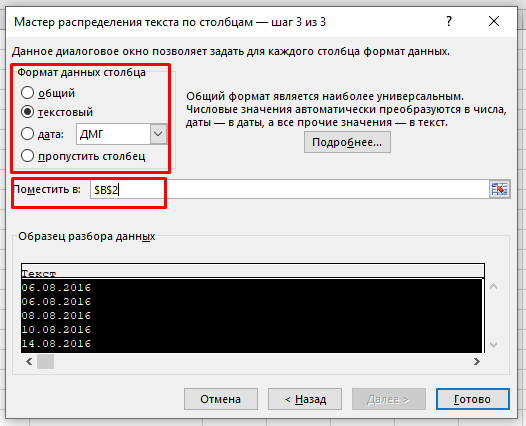
Функция сразу же переводит даты в текстовый формат.
Важная информация: эта функция устанавливает формат для дат по умолчанию для настроек вашей системы. То есть если вы хотите записать даты в определенном формате вам нужно использовать способы рассмотренные ранее, но для начала дочитайте нашу статью, возможно следующий вариант подойдет вам.
Переводим дату в текстовый формат с помощью копирования и вставки
Пошаговая инструкция:
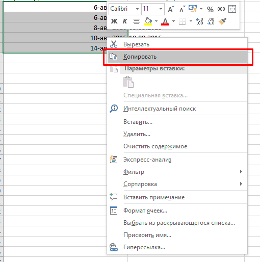
- Выделите ячейки с датами, которые нужно преобразовать, и скопируйте их;
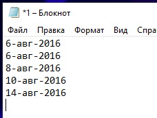
- Откройте обычный блокнот и вставьте наши данные туда, как только вы это сделаете, данные сразу же потеряют формат, т.е. станут обычным текстом (потому что в блокноте нет никаких форматов данных, кроме текста);
- Выделите ячейки, куда вы будете вставлять даты и поменяйте их формат на «Текстовый»;
- А теперь, заново скопируйте даты из блокнота, а затем вставьте их в Excel.
Excel сохраняет даты в виде порядковых номеров. Человеку невозможно их читать и понимать, но, таким образом, можно использовать их в функциях расчета, к примеру добавить к дате или времени какое-то количество времени (день, год и так далее).
Но, довольно часто, вам может быть нужно использовать даты в одних ячейках с текстом, так сказать, объединять.
На картинке пример объединения даты с текстом в одной ячейке. Видите как выглядит наша дата? Это формат порядкового номера Excel.
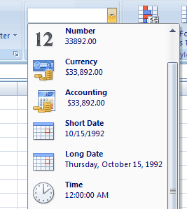
What is a date in Excel?
A date is a number! And like any number (currency, percentage, decimal, …), you can customize your date format 👍
Dates are whole numbers
Usually, when you insert a date in a cell it is displayed in the format dd/mm/yyyy or mm/dd/yyyy.
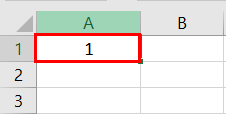
Let’s say you have the date 01/01/2016 in a cell. If you change the cell’s format to Standard, the cell displays 42370 😕🤔

Explanation of the numbering
In Excel, a date is the number of days since 01/01/1900 (the first date in Excel).
So 42370 is the number of days between 01/01/1900 and 01/01/2016.
Date format
Dates can be displayed in different ways using the following 2 options (available in the Number Format dropdown in the main menu):
- Short Date
- Long Date

How to customize a date?
To customize a date:
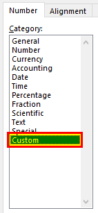
- Open the dialog box Custom Number (with the shortcut Ctrl + 1 or by clicking on the menu More number formats at the bottom of the number format dropdown)

- In this dialog box, you select ‘Custom‘ in the Category list and write the date format code in ‘Type‘.

To format a date, you just write the parameter d, m or y a different number of times. For example,
- dd/mm/yyyy will display 01/01/2016
- dd mmm yyyy => 01 Jan 2016
- mmmm yyyy => January 2016
- dddd dd => Friday 01
In function of your language , the letter could be different:
- t for «tag» (day) in German
- j for «jour» (day) in French
- a for «año» (year) in Spanish
Don’t write text in your cell !!!
With dates, one of the most common mistakes is to write text inside the format code (1 January 2016 for example). Never do this in Excel ⛔⛔⛔
If you do this, the contents of the cell will be Text and not a number
- In Excel, text is always displayed on the left of a cell.
- A number or a date is displayed on the right.

If you want to display the month in letters, just change the month format of your date.
Different examples of custom date
The following document shows you the same date but in different formats. The code for each date is in column A.

Different writing of dates according to the format code
In the following document, you can see the impact of each format on the same date.

What is the Date Format in Excel?
In Excel, a date is displayed according to the format selected by the user. One can choose from the different formats available or create a customized format according to the requirement. The default date format is specified in the “Control Panel” of the system. However, it is possible to change these default settings.
For example, the date 01/01/2021 corresponds to the format dd/mm/yyyy. If the format is changed to d-mmm-yyyy, the date becomes 1-Jan-2021.
We can change the date format in Excel either from the “Number Format” of the “Home” tab or the “Format Cells” option of the context menu.
In Excel for Windows, 1900 is the default date system. Whereas, in Excel for Mac, 1904 is the default date system. Both these systems store the dates as consecutive numbers having a difference of 1. These numbers are known as serial values or serial numbers. The reason dates are stored as serial numbers is to facilitate calculations.
In the 1900 date system, the first date that Excel recognizes is January 1, 1900. This date is stored as the number 1 in Excel. Consequently, the number 2 represents January 2, 1900. The last date recognized by Excel is December 31, 9999. It is represented by the serial number 2958465. Date before 1900 or after 9999 is identified as a text value by Excel.
Dates are stored only as positive integers in the 1900 date system. However, to display negative numbers as negative dates, one needs to switch to the 1904 date system.
In the 1904 date system, 0 represents January 1, 1904, and -1 means January -2, 1904. The number 1 represents January 2, 1904. The last date recognized by Excel (in the 1904 date system) is December 31, 9999, represented by the serial number 2957003.
In this article, we follow the 1900 date system.
Table of contents
- What is theDate Format in Excel?
- Code of Date Format in Excel
- How to Change Date Format in Excel?
- Example #1–Apply Default Format of Long Date in Excel
- Example #2–Change the Date Excel Format Using “Custom” Option
- Example #3–Apply Different Types of Customized Date Formats in Excel
- Example #4–Convert Text Values Representing Dates to Actual Dates
- Example #5–Change the Date Format Using “Find and Replace” Box
- Frequently Asked Questions
- Recommended Articles
Code of Date Format in Excel
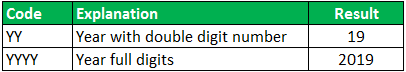
A code (like dd-mm-yyyy) is a representation of a day (d), month (m), and year (y). We can change the appearance of the date by changing the specified code.
The different codes, their explanation, and output (for days, months, and years) have been presented in the following images.
Notations for a Day

Notations for a Month

Notations for a Year
How to Change Date Format in Excel?
Here we look at some of the date format examples in Excel and how to change them.
Example #1–Apply Default Format of Long Date in Excel
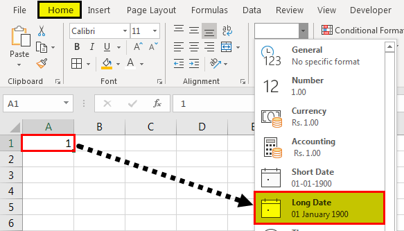
The following image shows a number in cell A1. We want to know the date represented by this number. The output should be in the long date format of Excel.
The steps to know the date represented by the number in cell A1 are listed as follows:
- We must first select cell A1. Then, from the “Home” tab, click the “Number Format” drop-down appearing in the “Number” section. Next, select “Long Date,” shown in the following image.

- The output is shown in the following image. The long date format displayed is dd mmmm yyyy. Hence, the number 1 represents the date 01 January 1900 in the long date format.
Note: The short and long dates appear as set in the “Control Panel.” Click “Clock, Language, and Region” in the “Control Panel” to change these default date formats. After that, click “Change date, time, or number formats.” Make the desired changes and click “OK.”
Likewise, had there been 2 in cell A1, the long date format would have been 02 January 1900. The number 3 would have been displayed as 03 January 1900 in the long date format.
Note: To switch to the 1904 date system, we must select “Advanced” from the “Options” of the “File” tab. Under “When calculating this workbook,” select “use 1904 date system” and click “OK.”

You can download this Change Date Format Excel Template here – Change Date Format Excel Template
Example #2–Change the Date Excel Format Using “Custom” Option
The following image shows some dates in the range A1:A6. These dates are in the format dd-mm-yyyy. We want to change their format to dd-mmmm-yyyy.
For instance, the date in cell A1 should appear as 25-February-2018. We may use the “Custom” option of the “Format Cells” dialog box.

The steps to change the date format in Excel are listed as follows:
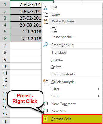
Step 1: We need to select all the dates of the range A1:A6. The same is shown in the following image.
Step 2: We must right-click the selection and choose “Format Cells” from the context menu. Alternatively, we may also press the keys “Ctrl+1” together.
Step 3: The “Format Cells” window opens, as shown in the following image.
Note: The default short date and long date formats are marked with an asterisk (*) in the box under “type.” The short date is 3/14/2012 (m/dd/yyyy), and the long date is Wednesday, March 14, 2012 (dddd, mmmm dd, yyyy).
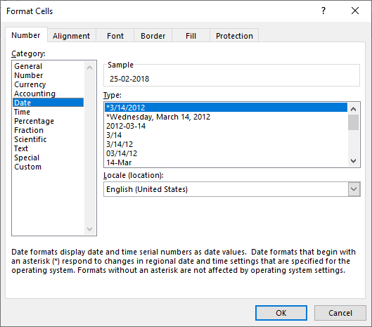
Step 4: From the “Number” tab, we need to select “Custom” under “Category.” The categories are shown on the left side of the “Format Cells” window.
Step 5: Under “Type,” we must insert the required date format. Either type the format (dd-mmmm-yyyy) or select it from the various options displayed in the box below “Type.”
Once the format has been entered, check the preview of the first date (of the range A1:A6) under “Sample.” The same is shown in the following image. Click “OK” in the “Format Cells” window if the date preview looks good.
Note 1: The date under “Sample” is displayed according to the format specified under “Type.”
Note 2: While creating custom date formats, we can use a forward slash (/), hyphen (-), comma (,), space ( ), etc.

Step 6: The output is shown in the following image. All dates of the range A1:A6 have been converted to the format dd-mmmm-yyyy. However, the Excel formula bar can still see the default date format. This default format corresponds with the short date set in the “Control Panel.”

Example #3–Apply Different Types of Customized Date Formats in Excel
The next image shows certain dates in the range A1:A6. At present, the date format is dd-mm-yyyy.
We want to apply four different formats to these dates. For using each format, the common steps to be performed are given as follows:
- First, we must select the range A1:A6.
- Then, right-click the selection and choose “Format Cells.”
- After that, from the “Number” tab, select “Custom” under “Category.”
Further, under each format, the additional steps to be performed followed by two images are given.

Format 1: dd-mmm-yyyy
- In the “Custom” option of the “Number” tab, select the format “dd-mmm-yyyy” under “Type.”
- Click “Ok.”

The output is given in the following image. All dates are displayed according to the format dd-mmm-yyyy. The hyphen is the separator between the day, month, and year in this format.

Format 2: dd mmm yyyy
- We must select the format “dd mmm yyyy” under “Type” of the “custom” option.
- Click “Ok.”

The output is given in the following image. All dates are converted to the format dd mmm yyyy. The space is the only separator between the day, month, and year in this format.

Format 3: ddd mmm yyyy
- In the “Custom” option, select the format “ddd mmm yyyy” under “Type.”
- Click “Ok.”

The output is given in the following image. The dates are shown in the format ddd mmm yyyy. The day and the month are displayed in their short notations in this format.

Format 4: dddd mmmm yyyy
- From the “Custom” option of the “Number” tab, select “dddd mmmm yyyy” under “Type.”
- Click “Ok.”

The output is given in the following image. All dates have been converted to the format dddd mmmm yyyy. The date, month, and year are displayed in their respective full forms in this format.

It must be observed that the date format changes as per the style set by the user. Therefore, the user can select a date format according to their convenience.
Example #4–Convert Text Values Representing Dates to Actual Dates
The following image shows a list of dates in the range A1:A6. At present, these dates are appearing as text values. We want to convert these text values to dates having the format dd-mmm-yyyy.

The steps to convert text values to dates having the given format are listed as follows:
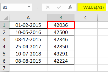
Step 1: First, enter the following formula in cell B1.
“=VALUE(A1)”
Then, press the “Enter” key.
Note 1: The VALUE functionIn Excel, the value function returns the value of a text representing a number. So, if we have a text with the value $5, we can use the value formula to get 5 as a result, so this function gives us the numerical value represented by a text.read more returns the numeric form of a text string that represents a number. In other words, it converts a number looking like the text into an actual number.
Note 2: Instead of the VALUE function, one can also use the DATEVALUE functionThe DATEVALUE function in Excel shows any given date in absolute format. This function takes an argument in the form of date text normally not represented by Excel as a date and converts it into a format that Excel can recognize as a date.read more of Excel. The latter converts a date stored as text to a serial number. This serial number is recognized as a date by Excel.
Step 2: We must select cell B1 and drag the fill handle until cell B6. The output is shown in the following image. All text values (A1:A6) have been converted to numbers (in the range B1:B6).
Ideally, the text string in Excel is left-aligned while the number string is right-aligned. However, we have centrally aligned both the ranges (A1:A6 and B1:B6).
Note: When text strings representing dates have been converted to serial values (or dates), we can use them for performing different calculations like addition, subtraction, and so on.
Step 3: To view the obtained serial numbers (in column B) as dates, apply the required format. We must select the range B1:B6, right-click and choose “Format Cells.”
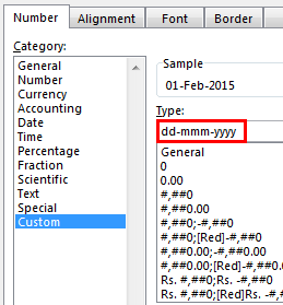
In the “Number” tab, select the option “Custom.” Then, under “Type,” enter or choose the format “dd-mmm-yyyy.” The same is shown in the following image.
If the sample date looks alright, click “OK.”
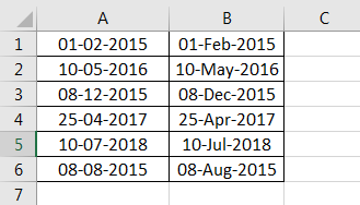
Step 4: The output is shown in the following image. Hence, all text values (of column A) have been converted to valid dates (in column B) having the format dd-mmm-yyyy.
Note: To ensure that a value is recognized as a date by Excel, check for the following signs:
- The dates are right-aligned as they are numerical values.
- If two or more dates are selected, the status bar (at the bottom of the worksheet) shows the count, average, numerical count, and sum. In addition, it may display one or more options according to the Excel version.
If a value is a text string, it would be left-aligned, and the status bar will show only the count.
Often, the Excel date format needs to be changed (from text to dates) when data is downloaded (or copied and pasted) from the web. That is because, in such instances, the dates may not be displayed as numbers.
Example #5–Change the Date Format Using “Find and Replace” Box
The following image shows some text values representing dates in the range A1:A6. The days, months, and numbers have been separated with a backslash. That is because we want to perform the following tasks:
- Replace all the backslashes () with forwarding slashes (/) by using the “Find and Replace” dialog box.
- Convert text values representing dates to actual dates.
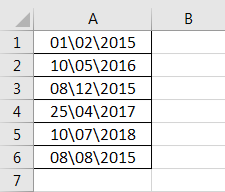
The steps to perform the given tasks are listed as follows:
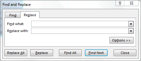
Step 1: We must press the keys “Ctrl+H” together. Then, the “find and replace” dialog box opens, as shown in the following image.
Step 2: Type a backslash in the “Find what” box (). In the “Replace with” box, type a forward slash (/).
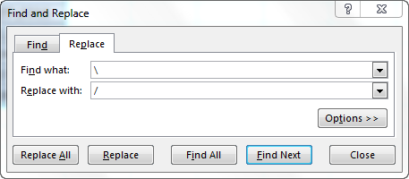
Step 3: Next, we must click “Replace All.” Excel shows a message stating the number of replacements it has made. Click “OK” to proceed. The final output is shown in the following image.
Hence, all backslashes have been replaced with forwarding slashes. With this replacement, the text values representing dates have automatically been converted to actual dates by Excel.
Since column A was aligned centrally from the beginning, this alignment is retained even after the values are converted to dates.

Frequently Asked Questions
1. How can the date format in Excel be changed?
The steps to change the date format in Excel are listed as follows:
The steps to change the date format in Excel are listed as follows:
a. Select the cell containing the date. If the date format of a range needs to be changed, select the entire range.
b. Right-click the selection and choose “Format Cells” from the context menu. Alternatively, press the keys “Ctrl+1” together.
c. IIn the “Number” tab, select the option “Date.” Next, select the required date format under “Type.”
d. Check the preview (of the first date of the selected range) under “Sample.” If the preview is good, click “OK.”
The date format of the selected cell or cells (selected in step a) is changed.
Note 1: The required date format may not be available under the “Date” option’s “Type.” If it is not available, select “Custom” as the “category” from the “Number” tab. Then, type the required date format under “Type” and click “OK.”
Note 2: If the selected cell (selected in step a) contains a text string representing a date, convert this string to date first. Then change the format to the desired date format.
2. How to change the date format permanently in Excel?
To change a date format permanently, one needs to make changes to the date formats of the “Control Panel.” That is because the short and long date formats of Excel reflect the date settings of the “Control Panel.”
The steps to change the date settings of the “Control Panel” are listed as follows:
We must open the “Control Panel” first from the “Start” menu.
b. In the “Clock, Language, and Region” category, click “Change date, time, or number format.” It is available under the “Region and Language” option.
c. The “Region and Language” or “Region” dialog box opens. Under “Format,” we must select the region.
d. Enter the required short and long date formats under “Date and Time Formats.” To enter customized short and long date formats, click “Additional Settings.” The “Customize Format” dialog box opens. Make the changes in the “Date” tab and click “OK.”
e. Check the preview under “Examples” at the bottom of the “Region and Language” box. If the preview is alright, click “OK.”
The default date settings have been changed. Now, we should enter a date in any format in Excel. Then select the short or the long date format from the “Number Format” (in the “Number” section) of the “Home” tab.
The dates will appear in the format set in the “Control Panel.” So, the user need not change the format of each date manually.
3. How to change a date to a text string in Excel?
Let us change the date 22/1/2019 in cell A1 to a text string in Excel. The text string should be in the format yyyy-mm-dd.
The steps to change a date to a text string are listed as follows:
a. First, we must enter the formula =TEXT(A1, “yyyy-mm-dd”) in cell B1.
b. Then, press the “Enter” key.
The date in cell A1 (22/1/2019) is converted to 2019-01-22 in cell B1. We must note that the date in cell A1 is right-aligned, being a number. In contrast, the text in cell B1 is left-aligned.
Note: The TEXT function helps convert numbers to text strings. It is used to display values in a specific format. The syntax is TEXT(value,format_text). “Value” is the number to be converted to text. “Format_text” is the format in which the number should be displayed.
Recommended Articles
This article has been a guide to the Date Format in Excel. We discuss changing and customizing date formats in Excel, practical examples, and a downloadable Excel template. You may also look at these useful functions in Excel: –
- Concatenate Columns in Excel
- Convert Date to Text in Excel
- Insert Date in Excel
- Concatenate Date in Excel
If you use Excel regularly, I’m sure you’ve come across dates and times in your cells. Data often has a record of when it was created or updated, so knowing how to work with this data is essential.
Here are three key skills that you’ll learn in this tutorial:
- How to format dates in Excel so that they appear in your preferred style
- Formulas to calculate the number of days, months, and years between two dates
- An Excel date formula to log today’s date, and a keyboard shortcut to add the current time
Microsoft Excel can basically do anything with data, if you just know how. This tutorial is another key step to adding skills to your Excel toolbelt. Let’s get started.
Excel Date and Time Formulas (Quick Video Tutorial)
This screencast will walk you through how to work with dates and times in Excel. I cover formatting dates to different styles, as well as Excel date formulas to calculate and work with dates. Make sure to download the free Excel workbook with exercises that I’ve attached to this tutorial.
Keep reading for a written reference guide on how to format dates and times in Excel, and work with them in your formulas. I’ll even share several tips that weren’t covered in the screencast.
Typing Dates and Times in Excel
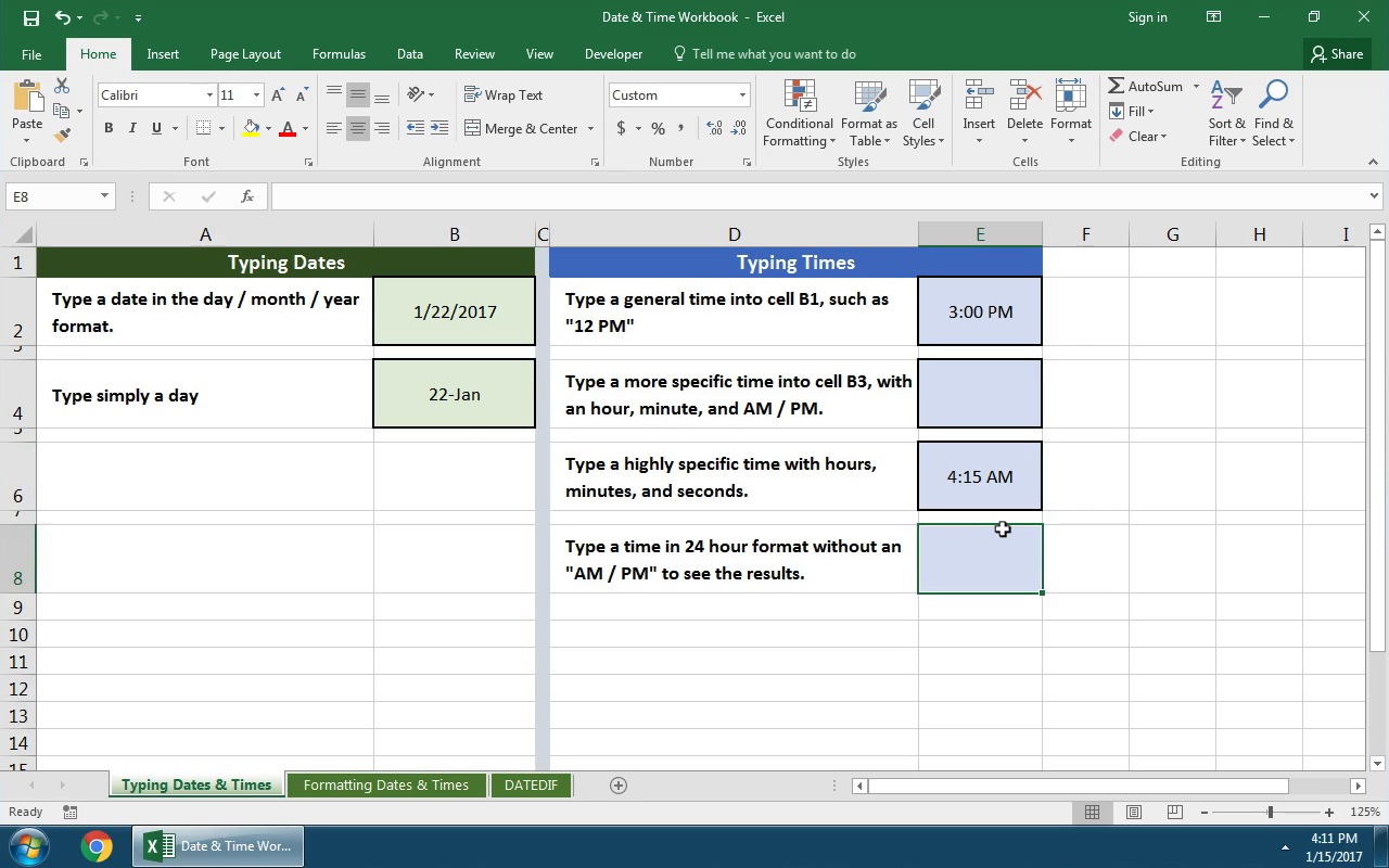
For this part of the tutorial, use the tab titled «Typing Dates & Times» in the example workbook.
One of the keys to working with dates and times in Excel is capturing the data correctly. Here’s how to type dates and times in your Excel spreadsheets:
1. How to Type Dates
I recommend typing dates in the same format that your system uses. For our American readers, a full date would be in the «day/month/year» format. European style dates are «month/day/year.»


When I’m typing dates, I always type in the full date with the month, day and year. If I only want to show the month and the year, I’ll simply format it that way (more on that in a minute.)
2. How to Type Times
It’s easy to type times in Excel. We can specify anything from just an hour of the day, to the exact second that something took place.
If I wanted to log the time as 4PM, I’d type «4 pm» into a cell in Excel and then press enter:


Notice once we press enter, Excel converts what we’ve typed into a hours : minutes: seconds data format.
Here’s how to log a more specific time in your spreadsheet:


The key is to use colons to separate the section of the time data, and then add a space plus «AM» or «PM.»
3. How to Type Date-Time Together
You can also type combinations of dates and times in Excel for highly specific timestamps.
To type a date-time combination, simply use what we’ve already learned about typing dates, and typing times.


Notice that Excel has converted the time to a 24 hour format when it’s used in conjunction with a date, by default. If you want to change the style of this date, keep reading.
Bonus: Excel Keyboard Shortcut for Current Time
One of my favorite Excel keyboard shortcuts inserts the current time into a spreadsheet. I use this formula often, when I’m noting the time I made a change to my data. Try it out:
Control + Shift + ;
Formatting Dates in Excel
For this part of the tutorial, use the tab titled «Formatting Dates & Times» in the example workbook.
What can you do when your dates are European style dates? That is, they’re in a day-month-year format, and you need to convert them to the more familiar month-day-year format?

In the screenshot above, what might surprise you is that all six of those cells contain exactly the same data — «1/22/2017.» What differs is how they’re formatted in Excel. The original data is identical, but it can be formatted to show in a variety of ways.
In most cases, it’s better to use formatting to modify the style of our dates. We don’t need to modify the data itself — just change how it’s presented.
Format Excel Cells
To change the appearance of our date and time data, make sure that you’re working on the Home tab of Excel. On the Ribbon (menu at the top of Excel), find the section labeled Number.
There’s a small arrow in the lower right corner of the section. Click it to open the Format Cells menu.


The Format Cells menu has a variety of options for styling your dates and times. You could turn «1/22/2017» into «Sunday, January 22nd» with just formatting. Then, you could grab the format painter and change all of your cell styles.


Spend some time exploring this menu and trying out the different styles for your Excel dates and times.
Get Data From Dates and Times
Let’s say that we have a list of data that has very specific dates and times, and we want to get simpler versions of those formulas. Maybe we have a list of exact transaction dates, but we want to work with them at a higher level, grouping them by year or month.
You can get the year from a date with this Excel formula:
=YEAR(CELL)


To get just the month from a date cell, use the following Excel formula:
=MON(CELL)


Find the Difference Between Dates and Times
For this part of the tutorial, use the tab titled «DATEDIF» in the example workbook.
While formats are used to change how dates and times are presented, formulas in Excel are used to modify, calculate, or work with dates and times programatically.
The DATEDIF formula is powerful for calculating differences between days. Give the formula two dates and and it will return the number of days, months, and years between two dates. Let’s look at how to use it.
1. Days Between Dates
This Excel date formula will calculate the number of days between two dates:
=DATEDIF(A1,B1,"d")
The formula takes two cells, separated by commas, and then uses a «d» to calculate the difference in days.


Here are some ideas for how you could use this Excel date formula to your advantage:
- Calculate the difference between today and your birthday to start a birthday countdown
- Use a DATEDIF to calculate the difference between two dates and divide your stock portfolio’s growth by the number of days to calculate the growth (or loss!) per day
2. Months Between Dates
DATEDIF also calculates the number of months between two dates. This date formula in Excel is very similar, but substitutes an «m» for «d» to calculate the difference in months:
=DATEDIF(A1,B1,"m")
However, there’s a quirk in the way Excel applies DATEDIF: it calculates whole months between dates. See the screenshot below.


To me, there are three months between January 1st and March 31st (all of January, all of February, and almost all of March.) However, because Excel uses whole months, it only considers January and February as completed, whole months, so the result is «2.»
Here’s my preferred way to calculate the number of months between two dates. We’ll find the date difference in days, and then divide it by the average number of days in a month — 30.42 .
=(DATEDIF(A1,B1,"d")/30.42)
Let’s apply our modified DATEDIF to two dates:


Much better. The output of 2.99 is very close to 3 full months, and this will be much more useful in future formulas.
The official Excel documentation has a complex method to calculate months between dates, but this is a simple and easy way to get it pretty close. Writing a good Excel formula is about finding the sweet spot of precision and simplicity, and this formula does both.
3. Years Between Dates
Finally, let’s calculate the number of years between two dates. The official way to calculate years between dates is with the following formula:
=DATEDIF(A1,B1,"y")
Notice that this is the same as our past DATEDIF formulas, but we’ve simply substituted the last part of the formula with «y» to calculate the number of years between two dates. Let’s see it in action:


Notice that this works like the DATEDIF for months: it counts only full years that have passed. I’d rather include partial years passing as well. Here’s a better DATEDIF for years:
=(DATEDIF(A1,B2,"d")/365)
Basically, we’re just getting the date difference in days, and then dividing it by 365 to calculate it as a year. Here’s the results:


DATEDIF is extremely powerful, but watch out for how it works: it’s going to only calculate full months or years that have passed by default. Use my modified versions for more precision in the results.
Bonus: Work Days Between Dates
The Excel date formulas covered above focus on the number of business days between dates. However, it’s sometimes helpful to just calculate the number of workdays (basically weekdays) between two dates.
In this case, we’ll use =NETWORKDAYS to calculate the number of workdays between two dates.
=NETWORKDAYS(A1,B1)
In the screenshot below, I show an example of using NETWORKDAYS. You can see the calendar showing how the formula calculated a result of «4.»


If you have known holidays in the timeframe that you want to exclude, check out the official NETWORKDAYS documentation.
Recap and Keep Learning
Dates and times are ubiquitous to spreadsheets. Excel date formulas and formatting options are helpful. The techniques in this tutorial can take your Excel skills to the next level so that you can incorporate date-driven data seamlessly into your spreadsheets.
You’ve added one skill to your Excel toolbox — why stop here? Chain Excel formulas and skills to create powerful spreadsheets. To keep learning more about working with Excel spreadsheets, check out these other resources:
- IF Statements are logic built into your spreadsheet that show results based on conditions. You could combine an IF Statement with a date range to show data based on a date or time. Check out this tutorial to learn them.
- You could combine the VLOOKUP tutorial with date and time formulas to match values based on a date or time.
- Find and Remove Duplicates is an Excel function used in combination with date and time data, as it’s often one of the best bits of data to check for duplicates.
How do you work with calendar and time data in your Excel spreadsheets? Are there are any Excel date or time formulas that I’m missing from this tutorial that you use regularly? If so, let me know in the comments.
If you are storing dates in Excel worksheets, the default format picked by the Excel is the format set in Control Panel. So, if your control panel setting is “M/d/yyyy”, the Excel will format the 2nd Feb 2010 date as follows:
2/2/2010
If you require displaying the date like 2-Feb-2010 or August 1, 2015, etc. as entering dates you may change the settings in Excel easily.
In case you require permanently changing the date format that applies to current as well as future work in Excel, you should change this in the control panel.
If you try entering a date like this: 20/2/2010 then Excel will take it as text because you provided day first for the default M/d/yyyy format.
For the current worksheet, you may set the date formatting in different ways as described in the following section with examples.
Related Learning: Add / Subtract Dates in Excel
First Way: Change the date format by “Format Cell” option
The first way I am going to show you for changing the date format in Excel is using the “Format Cells” option. Follow these steps:
Step 1:
Right click on a cell or multiple cells where you require changing the date format. For the demo, I have entered a few dates and selected all:
Click the “Format Cells” option that should open the Format Cells dialog. You may also press the Ctrl+1 for opening this dialog in Windows. For Mac, the short key is Control+1 or Command+1.
Step 2:
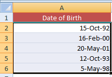
In the Format Cells dialog, the Number tab should be pre-selected. If not, press Number tab. Under the Category, select Date. Towards the right side, you can see Type.
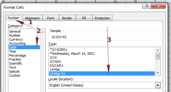
For the demo, I have selected 14-Mar-01 format and press OK. The resultant sheet after modifying date format is:
You are done!
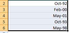
An example of Mon-year format
The following example displays the dates in Mon-Year format e.g. Oct-92. For that, open the “Format Cells” dialog again –> Number –> Date and select Mar-01 format.
The above sheet displays the same dates as shown below:
Similarly, you may choose any date format as per the requirement of your scenario.
Interesting Topic: How to calculate age in Excel
Change date format by locale/location
If you wish to display the dates based on other languages then you may use the Locale (location) option in the “Format Cells” dialog.
See the following Excel sheet where I set the Arabic(UAE) option and one of its type:
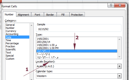
The resultant sheet for the same dates as in the above examples:
Similarly, you may choose the following locale:
- Bashkir (Russia)
- Chinese (Simplified, Singapore)
- Corsican (France)
- Danish (Denmark)
- Various options for English
- Hindi (India)
- Japanese (Japan)
- And many more
Customizing the date format
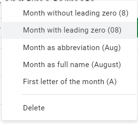
By using the date formatting codes, you may customize the dates in a flexible way. For example, displaying the short month name (Jan, Feb) by using “mmm” or full month name by “mmmm”.
Similarly, showing the day names of the Week (Sun, Mon) by ddd or full names (Sunday, Monday) by dddd formatting code.
First, have look at an example of customizing the date which is followed by the list of date formatting codes.
Select and right click on date cells that you want to customize and go to “Format Cells”. Under the Number –> Category, select Date and choose the closest format you wish to display e.g. “Mar 14, 2001”.
Under the Category, press Custom now and towards the right side, you should see Type with various options. Either choose a format from the available list or enter the formatting code as required in the text box under Type.
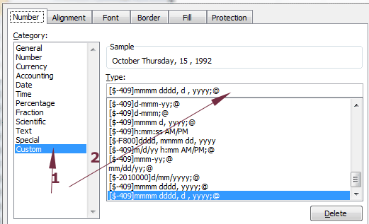
For the example, I entered the “[$-409]mmmm dddd, d , yyyy;@” and see the resultant sheet:
List of formatting codes in Excel
Following is the formatting code list that you may use to customize the dates:
Day Codes
- d – for the day as 1-31
- dd – for the day as 01-31
- ddd – Sun, Mon, Tue
- dddd – Sunday, Monday, Tuesday etc.
Month Codes
- m – for Months as 1-12
- mm – 01-12
- mmm – Apr, May, Jun etc.
- mmmm – April, May, June, July etc.
- mmmmm – Month as the first letter of the month
Year Codes
- yy – 00-99
- yyyy – 2000, 2002, 2010 etc.
You may also want to learn: Convert Number and Date to Text
Quick way of displaying dates in default short and long formats
If you need to display dates in the short or long format with default settings, you may do it by following this:
Select the dates you wish to format in short/long date formats. For that, I chose the above example dates that were formatted in the custom format (see the last graphic):
Now, go to the Home tab and in the Number group, click the Number Format box as shown below:
Press the Short Date or Long Date format.
Changing date format in Excel by TEXT function
The Excel TEXT function can also be used for formatting dates. The TEXT function takes two arguments as shown below:
=TEXT(Value to convert into text, “Formatting code “)
Where the first argument can be a date cell, a number etc.
The second argument should sound familiar now; the formatting code that we just learned.
The TEXT function for formatting dates can particularly be useful if you want to keep the original date column in place and displaying another date-set based on those dates.
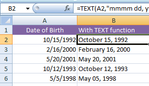
An example of Full month, day and year formatting example
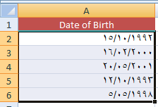
For the example, the A column cells are assigned the Date of Birth dates in default format (US English) i.e. M/d/yyyy.
The corresponding B cells will display the dates in full month name, day and year in four digits format.
The TEXT formula:
=TEXT(A2,«mmmm dd, yyyy»)
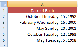
The resultant sheet with formatted dates:
I have written the formula in the B2 cell only and copied to B6 cell as follows.
After you get the result in B2 cell by writing the above formula, bring the mouse over the right bottom of the B2 cell. As + sign appears with solid line, drag the handle till B6 and formula should be copied to other cells. The Excel will update the corresponding A cells with respect to B cells automatically.
How to use the DATEDIF function in Excel
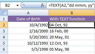
Formatting dates in d, mmm, yy by TEXT function
The following example displays the dates in day with leading zero (01-12), short month name and year in two-digit format.
The TEXT formula:
The resultant sheet:
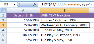
Displaying the day name as well
See the example below where day name (Sunday, Monday etc.) is also displayed along with day without leading zero, full month name and year in four digits.
The formula:
=TEXT(A2,«dddd d mmmm, yyyy»)
The dates after formatting:
The TEXT function is more than formatting dates; this is just one usage that I explained in above section. You may learn more about this function: The TEXT function in Excel
The example of concatenating formatted dates
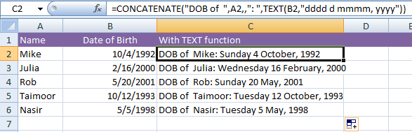
Let us get more comfortable with date formatting and create more useful text strings as a result of joining different cells with constant literals.
In the example below, column A contains Names and column B date of births. In column C, I will use the CONCATENATE function where a text string is used and corresponding A and B cells are joined in the formula as follows:
=CONCATENATE(«DOB of «,A2,,«: «,TEXT(B2,«dddd d mmmm, yyyy»))
This is what we get:
Formatting dates specific to language by TEXT function
As we have seen in the custom date formatting example, you can display Locale specific date style. I showed an example of displaying dates in Arabic style by using custom date option in “Format cells” dialog.
You may also specify the language code in the TEXT function for displaying dates based on locales.
See the following example where I displayed dates in various languages by using TEXT function.
The resultant sheet:
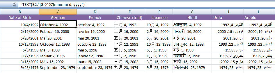
The following formulas are used for different languages:
For German:
=TEXT(B2,«[$-0407]mmmm d, yyyy»)
French:
=TEXT(B2,«[$-0040C]mmmm d, yyyy»)
Chinese (Traditional):
=TEXT(B2,«[$-0804]mmmm d, yyyy»)
Japanese:
=TEXT(B2,«[$-0411]mmmm d, yyyy»)
Arabic:
=TEXT(B2,«[$-0401]mmmm d, yyyy»)
For Hindi:
=TEXT(B2,«[$-0439]mmmm d, yyyy»)
Urdu:
=TEXT(B2,«[$-0420]mmmm d, yyyy»)
List of language codes
Following is the list of language codes that you may use in the TEXT function for locale-specific date formatting:
Lang. Code Language
- 042B Armenian
- 044D Assamese
- 082C Azeri (Cyrillic)
- 042C Azeri (Latin)
- 042D Basque
- 0423 Belarusian
- 0445 Bengali
- 0402 Bulgarian
- 0804 Chinese (Simplified)
- 0404 Chinese (Traditional)
- 041A Croatian
- 0405 Czech
- 0406 Danish
- 0413 Dutch
- 0C09 English (Australian)
- 1009 English (Canadian)
- 0809 English (U.K.)
- 0409 English (U.S.)
- 0464 Filipino
- 040B Finnish
- 040C French
- 0C0C French (Canadian)
- 0462 Frisian
- 0467 Fulfulde
- 0456 Galician
- 0437 Georgian
- 0407 German
- 0C07 German (Austrian)
- 0807 German (Swiss)
- 0408 Greek
- 0447 Gujarati
- 040D Hebrew
- 0439 Hindi
- 040E Hungarian
- 0421 Indonesian
- 0410 Italian
- 0411 Japanese
- 044B Kannada
- 0460 Kashmiri (Arabic)
- 0412 Korean
- 0476 Latin
- 0426 Latvian
- 0427 Lithuanian
- 042F Macedonian FYROM
- 043E Malay
- 044C Malayalam
- 043A Maltese
- 0458 Manipuri
- 044E Marathi
- 0450 Mongolian
- 0461 Nepali
- 0414 Norwegian Bokmal
- 0463 Pashto
- 0429 Persian
- 0415 Polish
- 0416 Portuguese (Brazil)
- 0816 Portuguese (Portugal)
- 0446 Punjabi
- 0418 Romanian
- 0419 Russian
- 044F Sanskrit
- 0C1A Serbian (Cyrillic)
- 081A Serbian (Latin)
- 0459 Sindhi
- 045B Sinhalese
- 041B Slovak
- 0424 Slovenian
- 0477 Somali
- 0C0A Spanish
- 0441 Swahili
- 041D Swedish
- 045A Syriac
- 0428 Tajik
- 045F Tamazight (Arabic)
- 085F Tamazight (Latin)
- 0449 Tamil
- 044A Telugu
- 041E Thai
- 041F Turkish
- 0442 Turkmen
- 0422 Ukrainian
- 0420 Urdu
- 0843 Uzbek (Cyrillic)
- 0443 Uzbek (Latin)
- 042A Vietnamese
- 0478 Yi
- 046A Yoruba
The example of calculating age in Years/Months and days
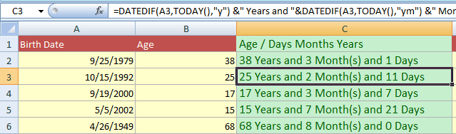
The following example uses the DATEDIF function for calculating the difference between current date and date of birth.
The current date is retrieved by using the TODAY() function. The Birth Date is stored in A column. The C column displays the formatted age in years, months and number of days.
The DATEDIF formula:
=DATEDIF(A3,TODAY(),«y») &» Years and «&DATEDIF(A3,TODAY(),«ym») &» Month(s) and « &DATEDIF(A3,TODAY(),«md») &» Days»
The resultant sheet:
For learning about the DATEDIF function, visit this tutorial: Excel DATEDIF function and formulas.

You are not limited to using Excel’s built-in date formats. You can create your desired custom date formats in more than one way. You can even display your dates in a different language, change the appearance and order in which your dates are shown, add display color, and much more. In this article, you can learn how to format dates using a built-in format and how to format dates with use of the TEXT() function.
Using the DATE function available in Microsoft Excel is pretty simple as the function itself is very intuitive and self-explanatory. This function requires several variables to work, such as year, month and day, which can be inserted directly or entered as references to other cells with these variables. The Date function has the following syntax: DATE( year, month, day ). I have used the DATE function in many of my Calendars Templates, Project Gantt Chart, etc.
The DATE function can be used as a part of other functions or custom formulas and can also use other functions within for entering required variables. For example, one of the commonly used together with DATE functions is TODAY(), which returns the current date and can be used inside the DATE function and make it more dynamic.
The question that I have often been asked is how to format dates in the cell to display dates in alphanumerical format? Another issue is how to format dates using the TEXT() function? Additionally, why the date that is shown is either partly correct or displaying error when the spreadsheet is used in the non-English version of Microsoft Excel?
Examples
To follow along and see the examples described on this page in action, download the Excel file below.
Download the Example File (custom-date-formats.xlsx)
Change the Date Appearance with Format Cells Option
There a few methods in which you can approach these problems. The first method applies to scenarios where the content of the cell has to be displayed in some specific way, or you want to enter custom formatting. You can easily format the cell to show the date the way you need by following these steps:
- Select the cell (or multiple cells) you want to format
- Right-click on a cell (or cells) and select “Format Cells…” or use Ctrl+1 shortcut
- In the Format Cells dialog box choose the Date from the categories on the left
- Using the Locale drop-down list, choose a country or region of the date format you want to use
- Choose the desired format type in the Type section, then click OK to apply the format

The steps to apply custom formatting to the date entered into a cell or multiple cells are very similar.
- Select the cell (or multiple cells) you want to format
- Right-click on a cell (or cells) and select “Format Cells…” or use Ctrl+1 shortcut
- In the Format Cells window choose Custom from the categories on the left
- Select the desired formatting from the list in the Type section or enter your custom format type

I won’t go through all custom formatting types that can be entered here as there are quite a few of them and it is quite frankly outside the scope of this article, but I will briefly touch upon the few of them. If you want to learn about all possible formatting types that you can create in Excel, please let me know in the comments below.
Here are some Date Format examples:
| Format Code | Cell Value | Cell Appearance |
|---|---|---|
| dd/mm/yyyy | 16/11/2018 | 16/11/2018 |
| mm/dd/yyyy | 16/11/2018 | 11/16/2018 |
| mm-dd-yy | 16/11/2018 | 11-16-18 |
| mmmm d, yyyy | 16/11/2018 | November 16, 2018 |
| d mmmm yyyy | 16/11/2018 | 16 November 2018 |
| d mmmm yyyy (dddd) | 16/11/2018 | 16 November 2018 (Friday) |
| mm•dd•yyyy | 16/11/2018 | 11•16•2018 |
| “Date:” d mmmm yyyy | 16/11/2018 | Date: 16 November 2018 |
You can enter your custom format type by clicking in the area as shown on the image above. For example, if you want to display the date as November 16, 2018, you would enter the following: mmmm dd, yyyy. Check the table below for more date format options.
| Format Code | Description |
|---|---|
| dddd | Full day of week names displayed as Monday-Sunday |
| ddd | Abbreviated day of week names displayed as Mon-Sun |
| dd | Days displayed with leading 0 as 01-31 |
| d | Days displayed as 1-31 |
| mmmmm | First letter of the month J-D |
| mmmm | Month Names displayed in full as January-December |
| mmm | Abbreviated month name displayed as Jan-Dec |
| mm | Month number displayed with leading 0 as 01-12 |
| m | Month number displayed as 1-12 |
| yyyy | Year displayed in four digit format: 2018, 2019, etc. |
| y or yy | Year displayed in two digit format: 18, 19, etc. |
In this table, you can view some examples that you can apply to change the appearance of the date in the cell.
| Format Code | Date Appearance |
|---|---|
| d mmm ddd | 6 Sep Thu |
| d mmm dddd | 6 Sep Thursday |
| d mmm yyyy (dddd) | 6 Sep 2018 (Thursday) |
| d mmm | 6 Sep |
| d mmmm | 6 September |
| dd/mm/yyyy | 06/09/2018 |
| dd-mm-yyyy | 06-09-2018 |
| d/m/yy | 6/9/18 |
| m/d/y | 9/6/18 |
| d mmm yy | 6 Sep 18 |
| mmm d, yy | Sep 6, 18 |
| d mmmm yyyy | 6 September 2018 |
| mmmm d, yyyy | September 6, 2018 |
| [$-C0A]mmmm d, yyyy | febrero 6, 2018 (Spanish) |
Additionally, the date can also appear in a different language by applying the language code to your formatting. For example, if you use the following language code [$-413] for Dutch, your date will appear in the Dutch language despite the system language settings of your computer. Language format can come in very handy, especially for use in spreadsheets where you want to display dates in various languages. I have posted the table with all applicable language codes at the bottom of this article.
All custom formatting applied via Excel built-in cell format option can be overwritten by conditional formatting or by accidental changes.
Format Dates with TEXT Function in Excel
If you are using the TEXT() function in your spreadsheet as a part of a formula or on its own, for applying a custom format to the date output, you can set the desired format right within the TEXT() function. To instruct the TEXT() function, you can use the same code that I have provided in the table above.
=TEXT(A1,"mmmm d, yyyy")
The formula above assumes that the date is in A1 (9/10/2018). The TEXT() function will apply the specified format to its output regardless of the initial format of the A1. So you should end up with the following output: September 9, 2018.
The output of the TEXT() function with a specified format cannot be changed with conditional formatting, which could sometimes be very useful. For example, you may not want to allow any system changes to override the format of your spreadsheet, such as system language changes. TEXT() function provides the ability to lock your set formats and can, to some extent prevent changes in the output.
One of many pros of using TEXT() function for setting a format of the date is the ability to set the different language for the output. You do this by including the language code with brackets to the format string, as shown in the example below
=TEXT(A1,"[$-C0A]mmmm d, yyyy")
Besides, you can make the TEXT() function even more dynamic by taking format string out of the worksheet function and placing it into any cell, then reference that cell in the format portion of the TEXT() function. Now you can change the format of the date by modifying the format string in the cell, without altering the TEXT() function.
=TEXT(A1,C2)
The formula in the example above assumes that A1 contains date and C2 includes the desired format string. The output of the TEXT() function will change every time you modify the format string in C2.
Custom Date Formats for Chart Labels and Axes

As with almost everything else in Excel, few different methods can be used to apply a custom format to the dates in the chart axes and labels. The first method is to add the custom date format from the Format Axis pane. You should notice that the Linked to source box is unchecked.
You can also follow the other methods to add a custom format to the date. For example, you can modify the format of the data source first then apply this format to your chart axis by checking the Link to source box in Format Axis pane.
Any formats applied with TEXT() function to the data source whether in cells or chart axes, cannot be overridden.
Custom Location Codes for Dates
The table below includes all custom location codes for dates. You can use these location codes at the beginning of the format code string in square brackets for displaying month names and weekday names in other languages. The location/language code contains either three or four digits and/or letters, but if the leading digit is a zero, you do not need to include it.
| Format Code | Language/Location |
|---|---|
| 0436 | Afrikaans |
| 041C | Albanian |
| 045E | Amharic |
| 0401 | Arabic |
| 042B | Armenian |
| 044D | Assamese |
| 082C | Azeri (Cyrillic) |
| 042C | Azeri (Latin) |
| 042D | Basque |
| 0423 | Belarusian |
| 0445 | Bengali |
| 0402 | Bulgarian |
| 0403 | Catalan |
| 045C | Cherokee |
| 0804 | Chinese (Simplified) |
| 0404 | Chinese (Traditional) |
| 041A | Croatian |
| 0405 | Czech |
| 0406 | Danish |
| 0465 | Dhivehi |
| 0413 | Dutch |
| 0466 | Edo |
| 0C09 | English (Australian) |
| 1009 | English (Canadian) |
| 0809 | English (U.K.) |
| 0409 | English (U.S.) |
| 0425 | Estonian |
| 0438 | Faeroese |
| 0464 | Filipino |
| 040B | Finnish |
| 040C | French |
| 0C0C | French (Canadian) |
| 0462 | Frisian |
| 0467 | Fulfulde |
| 0456 | Galician |
| 0437 | Georgian |
| 0407 | German |
| 0C07 | German (Austrian) |
| 0807 | German (Swiss) |
| 0408 | Greek |
| 0447 | Gujarati |
| 0468 | Hausa |
| 0475 | Hawaiian |
| 040D | Hebrew |
| 0439 | Hindi |
| 040E | Hungarian |
| 0469 | Ibibio |
| 040F | Icelandic |
| 0470 | Igbo |
| 0421 | Indonesian |
| 045D | Inuktitut |
| 0410 | Italian |
| 0411 | Japanese |
| 044B | Kannada |
| 0471 | Kanuri |
| 0460 | Kashmiri (Arabic) |
| 043F | Kazakh |
| 0457 | Konkani |
| 0412 | Korean |
| 0440 | Kyrgyz |
| 0476 | Latin |
| 0426 | Latvian |
| 0427 | Lithuanian |
| 042F | Macedonian FYROM |
| 043E | Malay |
| 044C | Malayalam |
| 043A | Maltese |
| 0458 | Manipuri |
| 044E | Marathi |
| 0450 | Mongolian |
| 0461 | Nepali |
| 0414 | Norwegian Bokmal |
| 0814 | Norwegian Nynorsk |
| 0448 | Oriya |
| 0472 | Oromo |
| 0463 | Pashto |
| 0429 | Persian |
| 0415 | Polish |
| 0416 | Portuguese (Brazil) |
| 0816 | Portuguese (Portugal) |
| 0446 | Punjabi |
| 0418 | Romanian |
| 0419 | Russian |
| 044F | Sanskrit |
| 0C1A | Serbian (Cyrillic) |
| 081A | Serbian (Latin) |
| 0459 | Sindhi |
| 045B | Sinhalese |
| 041B | Slovak |
| 0424 | Slovenian |
| 0477 | Somali |
| 0C0A | Spanish |
| 0441 | Swahili |
| 041D | Swedish |
| 045A | Syriac |
| 0428 | Tajik |
| 045F | Tamazight (Arabic) |
| 085F | Tamazight (Latin) |
| 0449 | Tamil |
| 0444 | Tatar |
| 044A | Telugu |
| 041E | Thai |
| 0873 | Tigrigna (Eritrea) |
| 0473 | Tigrigna (Ethiopia) |
| 041F | Turkish |
| 0442 | Turkmen |
| 0422 | Ukrainian |
| 0420 | Urdu |
| 0843 | Uzbek (Cyrillic) |
| 0443 | Uzbek (Latin) |
| 042A | Vietnamese |
| 0478 | Yi |
| 043D | Yiddish |
| 046A | Yoruba |
Other Notes about Custom Date Formats
You can quickly delete any custom formats created with built-in Format Cells option. To do so, open the Format Cells dialog box, select Custom from the categories on the left, select the custom format from the list then click Delete then click OK. All values that use the custom format which you want to delete will revert to the General format.
All custom date formats that you create belong to the workbook in which they were created. You will have to recreate the custom formats again in the new workbook or copy/paste the formatting from the file where you have initially created them. You can achieve this by copying and pasting the formatted cell, by copying the format code and pasting this code into the Format Cells dialog box or by using the Format Painter tool.
References
- Excel Custom Number Format by Mynda Treacy, Excel MVP (MyOnlineTrainingHub.com)
- Excel TEXT Function by Dave and Lisa Bruns (ExcelJet.net)
Return to Excel Formulas List
Download Example Workbook
Download the example workbook
This tutorial will demonstrate how to change date formats in Excel and Google Sheets.
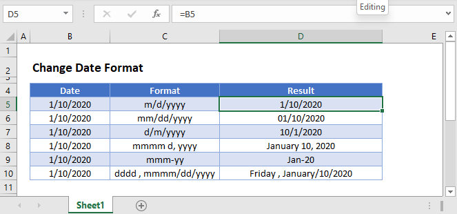
Excel Date Format
In spreadsheets, dates are stored as serial numbers, each whole number represents an unique day. When you type a date into a cell, the date is converted to it’s corresponding serial number and the number format is changed to date.
After a date is entered in Excel as a date, there are several ways to change the formatting:
Change Date Formats
Short Date / Long Date
The Ribbon Home > Number menu allows you to change between Short Dates (default) and Long Dates:
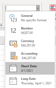
Format Cells Menu – Date
The Format Cells Menu gives you numerous preset formats:
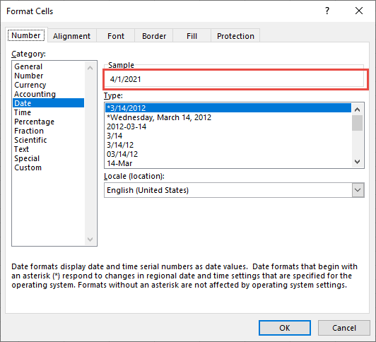
Notice that in the ‘Sample’ area you can see the impact the new number format will have on the active cell.
The Format Cells Menu can be accessed with the shortcut CTRL + 1 or by clicking this button:
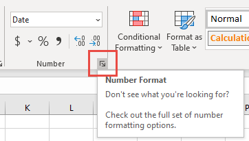
Custom Number Formatting
The Custom section of the Format Cells Menu allows you the ability to create your own number formats:
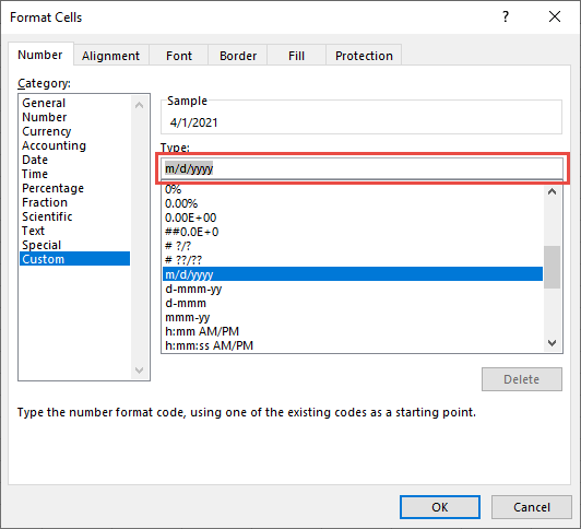
To set custom number formatting for dates, you’ll need to specify how to display days, months, and / or years. Use this table as guide:
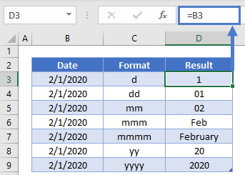
You can use the above examples to only display a day, month, or year. Or you can combine them:
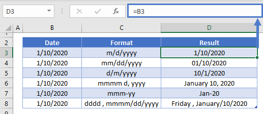
Dates Stored as Text
Date as Text
To store a date as text, type an apostrophe (‘) in front of the date as you’re typing the date:
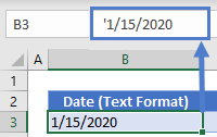
However, as long as the date is stored as text you’ll be unable to change the formatting like a normal date.
You can convert the date stored as text, back to a date using the DATEVALUE or VALUE Functions:
=DATEVALUE(B3)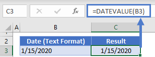
Text Function
The TEXT Function is a great way to display a date as text. The TEXT Function allows you to display dates in formats just like the Custom Number Formatting discussed previously.
=TEXT(B3,C3)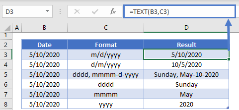
You can combine the TEXT Function with a string of text like this:
="Today's date is: "&TEXT(TODAY(),"m/d/yyyy")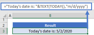
Google Sheets Date Formatting
Google Sheets makes formatting dates slightly easier. With Google Sheets, you simply need to navigate to the ‘More date and time formats:
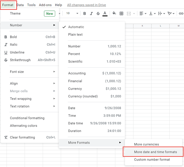
The menu looks like this:
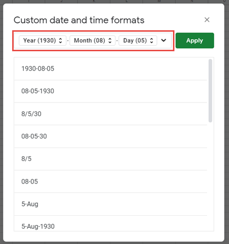
You’ll be able to select from a wide range of presets. Or you can utilize the drop-downs on top to select your desired format: