
Use the DATEDIF function when you want to calculate the difference between two dates. First put a start date in a cell, and an end date in another. Then type a formula like one of the following.
Warning: If the Start_date is greater than the End_date, the result will be #NUM!.
Difference in days
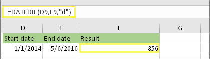
In this example, the start date is in cell D9, and the end date is in E9. The formula is in F9. The “d” returns the number of full days between the two dates.
Difference in weeks
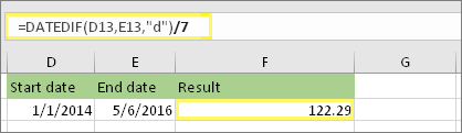
In this example, the start date is in cell D13, and the end date is in E13. The “d” returns the number of days. But notice the /7 at the end. That divides the number of days by 7, since there are 7 days in a week. Note that this result also needs to be formatted as a number. Press CTRL + 1. Then click Number > Decimal places: 2.
Difference in months

In this example, the start date is in cell D5, and the end date is in E5. In the formula, the “m” returns the number of full months between the two days.
Difference in years
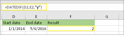
In this example, the start date is in cell D2, and the end date is in E2. The “y” returns the number of full years between the two days.
Calculate age in accumulated years, months, and days
You can also calculate age or someone’s time of service. The result can be something like “2 years, 4 months, 5 days.”
1. Use DATEDIF to find the total years.
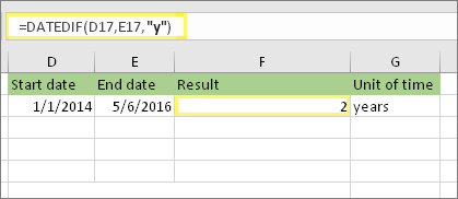
In this example, the start date is in cell D17, and the end date is in E17. In the formula, the “y” returns the number of full years between the two days.
2. Use DATEDIF again with “ym” to find months.
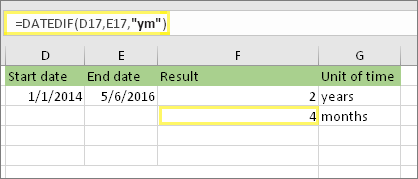
In another cell, use the DATEDIF formula with the “ym” parameter. The “ym” returns the number of remaining months past the last full year.
3. Use a different formula to find days.
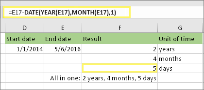
Now we need to find the number of remaining days. We’ll do this by writing a different kind of formula, shown above. This formula subtracts the first day of the ending month (5/1/2016) from the original end date in cell E17 (5/6/2016). Here’s how it does this: First the DATE function creates the date, 5/1/2016. It creates it using the year in cell E17, and the month in cell E17. Then the 1 represents the first day of that month. The result for the DATE function is 5/1/2016. Then, we subtract that from the original end date in cell E17, which is 5/6/2016. 5/6/2016 minus 5/1/2016 is 5 days.
Warning: We don’t recommend using the DATEDIF «md» argument because it may calculate inaccurate results.
4. Optional: Combine three formulas in one.
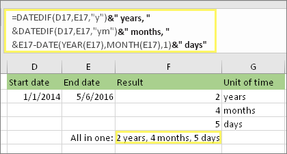
You can put all three calculations in one cell like this example. Use ampersands, quotes, and text. It’s a longer formula to type, but at least it’s all in one. Tip: Press ALT+ENTER to put line breaks in your formula. This makes it easier to read. Also, press CTRL+SHIFT+U if you can’t see the whole formula.
Download our examples
Other date and time calculations
As you saw above, the DATEDIF function calculates the difference between a start date and an end date. However, instead of typing specific dates, you can also use the TODAY() function inside the formula. When you use the TODAY() function, Excel uses your computer’s current date for the date. Keep in mind this will change when the file is opened again on a future day.
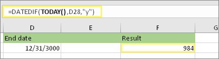
Please note that at the time of this writing, the day was October 6, 2016.
Use the NETWORKDAYS.INTL function when you want to calculate the number of workdays between two dates. You can also have it exclude weekends and holidays too.
Before you begin: Decide if you want to exclude holiday dates. If you do, type a list of holiday dates in a separate area or sheet. Put each holiday date in its own cell. Then select those cells, select Formulas > Define Name. Name the range MyHolidays, and click OK. Then create the formula using the steps below.
1. Type a start date and an end date.
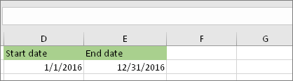
In this example, the start date is in cell D53 and the end date is in cell E53.
2. In another cell, type a formula like this:
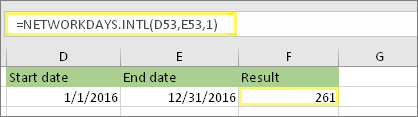
Type a formula like the above example. The 1 in the formula establishes Saturdays and Sundays as weekend days, and excludes them from the total.
Note: Excel 2007 doesn’t have the NETWORKDAYS.INTL function. However, it does have NETWORKDAYS. The above example would be like this in Excel 2007: =NETWORKDAYS(D53,E53). You don’t specify the 1 because NETWORKDAYS assumes the weekend is on Saturday and Sunday.
3. If necessary, change the 1.
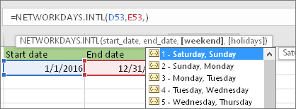
If Saturday and Sunday are not your weekend days, then change the 1 to another number from the IntelliSense list. For example, 2 establishes Sundays and Mondays as weekend days.
If you are using Excel 2007, skip this step. Excel 2007’s NETWORKDAYS function always assumes the weekend is on Saturday and Sunday.
4. Type the holiday range name.

If you created a holiday range name in the “Before you begin” section above, then type it at the end like this. If you don’t have holidays, you can leave the comma and MyHolidays out. If you are using Excel 2007, the above example would be this instead: =NETWORKDAYS(D53,E53,MyHolidays).
Tip: If you don’t want to reference a holiday range name, you can also type a range instead, like D35:E:39. Or, you could type each holiday inside the formula. For example if your holidays were on January 1 and 2 of 2016, you’d type them like this: =NETWORKDAYS.INTL(D53,E53,1,{«1/1/2016″,»1/2/2016»}). In Excel 2007, it would look like this: =NETWORKDAYS(D53,E53,{«1/1/2016″,»1/2/2016»})
You can calculate elapsed time by subtracting one time from another. First put a start time in a cell, and an end time in another. Make sure to type a full time, including the hour, minutes, and a space before the AM or PM. Here’s how:
1. Type a start time and end time.
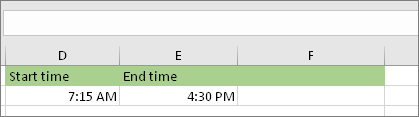
In this example, the start time is in cell D80 and the end time is in E80. Make sure to type the hour, minute, and a space before the AM or PM.
2. Set the h:mm AM/PM format.
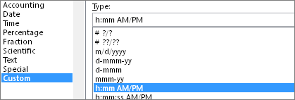
Select both dates and press CTRL + 1 (or  + 1 on the Mac). Make sure to select Custom > h:mm AM/PM, if it isn’t already set.
3. Subtract the two times.
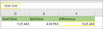
In another cell, subtract the start time cell from the end time cell.
4. Set the h:mm format.
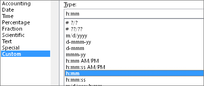
Press CTRL + 1 (or + 1 on the Mac). Choose Custom > h:mm so that the result excludes AM and PM.
To calculate the time between two dates and times, you can simply subtract one from the other. However, you must apply formatting to each cell to ensure that Excel returns the result you want.
1. Type two full dates and times.
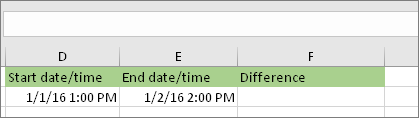
In one cell, type a full start date/time. And in another cell, type a full end date/time. Each cell should have a month, day, year, hour, minute, and a space before the AM or PM.
2. Set the 3/14/12 1:30 PM format.

Select both cells, and then press CTRL + 1 (or + 1 on the Mac). Then select Date > 3/14/12 1:30 PM. This isn’t the date you’ll set, it’s just a sample of how the format will look. Note that in versions prior to Excel 2016, this format might have a different sample date like 3/14/01 1:30 PM.
3. Subtract the two.
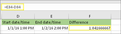
In another cell, subtract the start date/time from the end date/time. The result will probably look like a number and decimal. You’ll fix that in the next step.
4. Set the [h]:mm format.
![Format Cells dialog, Custom command, [h]:mm type](https://support.content.office.net/en-us/media/2edbd461-d4c5-49a7-a5a2-b6d9329c0411.png)
Press CTRL + 1 (or + 1 on the Mac). Select Custom. In the Type box, type [h]:mm.
Related Topics
DATEDIF function
NETWORKDAYS.INTL function
NETWORKDAYS
More date and time functions
Calculate the difference between two times
17 авг. 2022 г.
читать 1 мин
Мы можем использовать функцию DATEDIF() для вычисления разницы между двумя датами в Excel.
Эта функция использует следующий синтаксис:
=DATEDIF(Начальная_Дата, Конечная_Дата, Метрика)
куда:
- Start_Date: дата начала
- End_Date: Дата окончания
- Метрика: метрика для расчета. Варианты включают:
- «д»: дни
- «м»: Месяцы
- «г»: годы
Важно отметить, что эта функция не появится автоматически в Excel, пока вы полностью не введете =РАЗНДАТ( в одну из ячеек.
В следующих примерах показано, как использовать эту функцию для вычисления разницы между двумя датами в Excel.
Пример 1: разница в днях
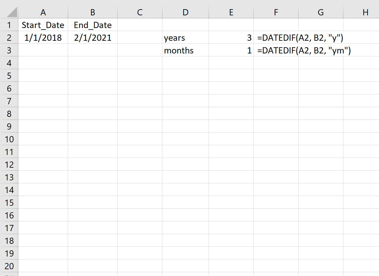
На следующем изображении показано, как рассчитать разницу (в днях) между двумя датами:
Это говорит нам о том, что между 01.01.2018 и 01.02.2021 1127 полных дней.
Пример 2: разница в месяцах
На следующем изображении показано, как рассчитать разницу (в месяцах) между двумя датами:
Пример 3: Разница в годах
На следующем изображении показано, как рассчитать разницу (в годах) между двумя датами:
Пример 4: Разница в годах и месяцах
На следующем рисунке показано, как рассчитать разницу (в годах и месяцах) между двумя датами:
Вы можете найти больше руководств по Excel на этой странице .
Написано
![]()
Замечательно! Вы успешно подписались.
Добро пожаловать обратно! Вы успешно вошли
Вы успешно подписались на кодкамп.
Срок действия вашей ссылки истек.
Ура! Проверьте свою электронную почту на наличие волшебной ссылки для входа.
Успех! Ваша платежная информация обновлена.
Ваша платежная информация не была обновлена.
We can use the DATEDIF() function to calculate the difference between two dates in Excel.
This function uses the following syntax:
=DATEDIF(Start_Date, End_Date, Metric)
where:
- Start_Date: The start date
- End_Date: The end date
- Metric: The metric to calculate. Options include:
- “d”: Days
- “m”: Months
- “y”: Years
It’s important to note that this function won’t automatically appear in Excel until you completely type =DATEDIF( into one of the cells.
The following examples show how to use this function to calculate the difference between two dates in Excel.
Example 1: Difference in Days
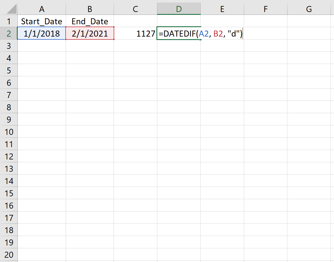
The following image shows how to calculate the difference (in days) between two dates:

This tells us that there are 1,127 full days between 1/1/2018 and 2/1/2021.
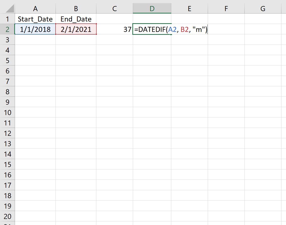
Example 2: Difference in Months
The following image shows how to calculate the difference (in months) between two dates:

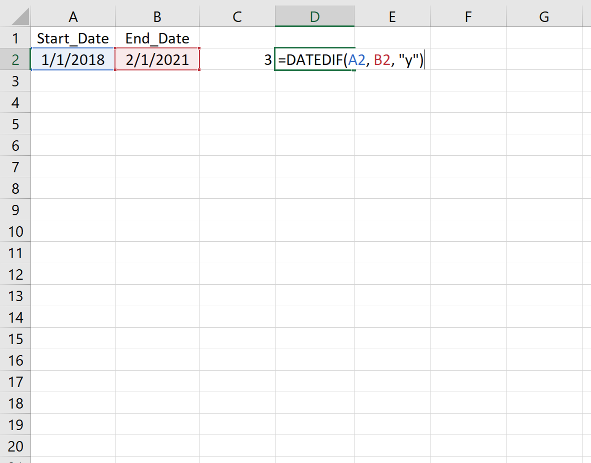
Example 3: Difference in Years
The following image shows how to calculate the difference (in years) between two dates:

Example 4: Difference in Years & Months
The following image shows how to calculate the difference (in years and months) between two dates:

You can find more Excel tutorials on this page.
This tutorial explains how to use Excel DATEDIF Function to calculate date difference (difference between two dates) in complete year, month or day.
You may also want to read:
Access Excel VBA day month year difference between two dates
DATEDIF function stands for “Date Difference“. It calculates the difference between two dates in complete year, month or day. Note that DATEDIF Function returns the “complete” value, for example, if the year difference between two dates is 1.99, the returned value is 1, not 2.
If you want to calculate the Date Difference in month / year in decimal places, use Days360 function, which has an assumption that each month has 30 days.
Syntax of Excel DATEDIF Function – calculate date difference
DATEDIF(start_date, end_date, format)
| start_date | Begin date, can be in text format (within double quote) or date serial (number) | ||||||||||||||
| end_date | End date, can be in text format or date serial | ||||||||||||||
| format | A text that specifies day/month/year difference (see below)
|
Example of Excel DATEDIF Function – calculate date difference
The dates in below examples are formatted in d/m/yyyy
| Formula | Result | Explanation |
| =DATEDIF(“1/9/2014″,”1/9/2014″,”D”) | 0 | 1-1=0 |
| =DATEDIF(“1/9/2013″,”31/8/2014″,”Y”) | 0 | Count 1 year if 31/8/2014 is passed. Calculation is based on complete year,no rounding or decimal places is returned |
| =DATEDIF(“1/9/2013″,”1/9/2014″,”Y”) | 1 | 2014-2013=1 |
| =DATEDIF(“1/7/2013″,”1/9/2014″,”YM”) | 2 | 9-7=2 |
| =DATEDIF(DATE(2013,7,1),DATE(2014,9,1),”YM”) | 2 | Express start_date and end_date in date serial |
Limitation of Excel DATEDIF Function – calculate date difference
DATEDIF Function returns an integer, it fails to convert the date difference to month with decimal places or year with decimal places.
In my another article, I will write a custom Function to solve this issue.
Alternative of Excel DATEDIF Function – calculate date difference
You can use Year Function, Month Function, and Day Function to extract the necessary information to calculate the difference
| Formula | Result | Explanation |
| =YEAR(A2)-YEAR(A1) | 2 | Year difference |
| =MONTH(A2)-MONTH(A1) | 5 | Month difference |
| =DAY(A2)-DAY(A1) | 10 | Day difference |
Outbound References
https://support.office.com/en-za/article/DATEDIF-function-bd549d1c-f829-4691-a77d-4a1e3d42bc1a
If you manage multiple projects, you would have a need to know how many months have passed between two dates. Or, if you’re in the planning phase, you may need to know the same for the start and end date of a project.
There are multiple ways to calculate the number of months between two dates (all using different formulas).
In this tutorial, I will give you some formulas that you can use to get the number of months between two dates.
So let’s get started!
Using DATEDIF Function (Get Number of Completed Months Between Two Dates)
It’s unlikely that you will get the dates that have a perfect number of months. It’s more likely to be some number of months and some days that are covered by the two dates.
For example, between 1 Jan 2020 and 15 March 2020, there are 2 months and 15 days.
If you only want to calculate the total number of months between two dates, you can use the DATEDIF function.
Suppose you have a dataset as shown below where you only want to get the total number of months (and not the days).
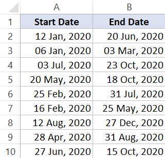
Below is the DATEDIF formula that will do that:
=DATEDIF(A2,B2,"M")
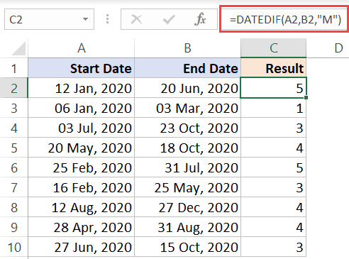
The above formula will give you only the total number of completed months between two dates.
DATEDIF is one of the few undocumented functions in Excel. When you type the =DATEDIF in a cell in Excel, you would not see any IntelliSense or any guidance on what arguments it can take. So, if you’re using DATEDIF in Excel, you need to know the syntax.
In case you want to get the total number of months as well as days between two dates, you can use the below formula:
=DATEDIF(A2,B2,"M")&"M "&DATEDIF(A2,B2,"MD")&"D"
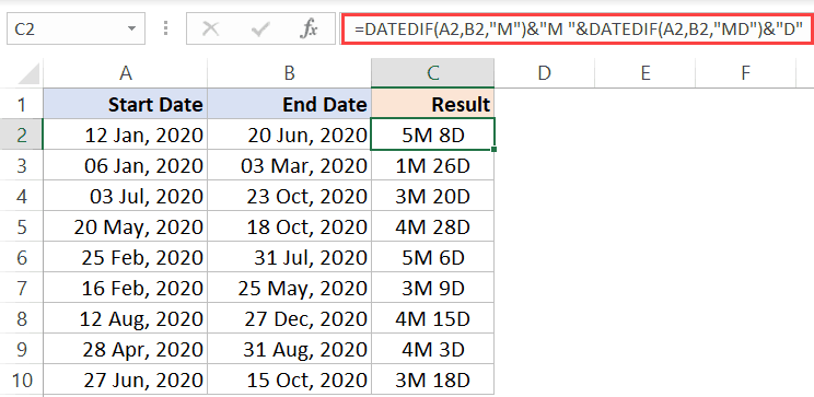
Note: DATEDIF function will exclude the start date when counting the month numbers. For example, if you start a project on 01 Jan and it ends on 31 Jan, the DATEDIF function will give the number of months as 0 (as it doesn’t count the start date and according to it only 30 days in January have been covered)
Using YEARFRAC Function (Get Total Months Between Two Dates)
Another method to get the number of months between two specified dates is by using the YEARFRAC function.
The YEARFRAC function will take a start date and end date as input arguments and it will give you the number of years that have passed during these two dates.
Unlike the DATEDIF function, the YEARFRAC function will give you the values in decimal in case a year has not elapsed between the two dates.
For example, if my start date is 01 Jan 2020 and end date is 31 Jan 2o20, the result of the YEARFRAC function will be 0.833. Once you have the year value, you can get the month value by multiplying this with 12.
Suppose you have the dataset as shown below and you want to get the number of months between the start and end date.
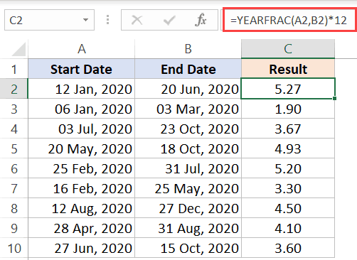
Below is the formula that will do this:
=YEARFRAC(A2,B2)*12
This will give you the months in decimals.
In case you only want to get the number of complete months, you can wrap the above formula in INT (as shown below):
=INT(YEARFRAC(A2,B2)*12)
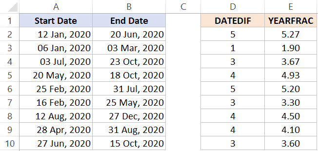
Another major difference between the DATEDIF function and YEARFRAC function is that the YEARFRAC function will consider the start date as a part of the month. For example, if the start date is 01 Jan and end date is 31 Jan, the result from the above formula would be 1
Below is a comparison of the results you get from DATEDIF and YEARFRAC.
Using the YEAR and MONTH Formula (Count All Months when the Project was Active)
If you want to know the total months that are covered between the start and end date, then you can use this method.
Suppose you have the dataset as shown below:
Below is the formula that will give you the number of months between the two dates:
=(YEAR(B2)-YEAR(A2))*12+MONTH(B2)-MONTH(A2)
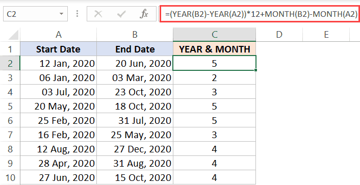
This formula uses the YEAR function (which gives you the year number using the date) and the MONTH function (which gives you the month number using the date).
The above formula also completely ignores the month of the start date.
For example, if your project starts on 01 Jan and ends on 20 Feb, the formula shown below will give you the result as 1, as it completely ignores the start date month.
In case you want it to count the month of the start date as well, you can use the below formula:
=(YEAR(B2)-YEAR(A2))*12+(MONTH(B2)-MONTH(A2)+1)
You may want to use the above formula when you want to know-how in how many months was this project active (which means that it could count the month even if the project was active for only 2 days in the month).
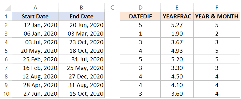
So these are three different ways to calculate months between two dates in Excel. The method you choose would be based on what you intend to calculate (below is a quick summary):
- Use the DATEDIF function method if you want to get the total number of completed months in between two dates (it ignores the start date)
- Use the YEARFRAC method when you want to get the actual value of months elapsed between tow dates. It also gives the result in decimal (where the integer value represents the number of full months and decimal part represents the number of days)
- Use the YEAR and MONTH method when you want to know how many months are covered in between two dates (even when the duration between the start and the end date is only a few days)
Below is how each formula covered in this tutorial will count the number of months between two dates:
Hope you found this Excel tutorial useful.
You may also like the following Excel tips and tutorials:
- How to Calculate the Number of Days Between Two Dates in Excel
- How to Remove Time from Date/Timestamp in Excel
- Convert Time to Decimal Number in Excel (Hours, Minutes, Seconds)
- How to Quickly Insert Date and Timestamp in Excel
- Convert Date to Text in Excel
- How to SUM values between two dates in Excel
- How to Add Months to Date in Excel
- How to Calculate Years of Service in Excel (Easy Formulas)
- How to Make an Interactive Calendar in Excel? (FREE Template)
The DATEDIF (Date + Dif) function is a «compatibility» function that comes from Lotus 1-2-3. For a long time, official documentation on DATEDIF was sparse. Even now (May 2021), Excel will not help you fill in arguments for DATEDIF like other functions. As the late Chip Pearson once wrote in his immortal words: DATEDIF is treated as the drunk cousin of the Formula family. Excel knows it lives a happy and useful life, but will not speak of it in polite conversation. Yet DATEDIF remains a very useful function for certain problems.
Time units
The DATEDIF function can calculate the time between a start_date and an end_date in years, months, or days. The time unit is specified with the unit argument, which is supplied as text. The table below summarizes available unit values and the result for each. Time units can be given in upper or lower case (i.e. «ym» is equivalent to «YM»).
| Unit | Result |
|---|---|
| «y» | Difference in complete years |
| «m» | Difference in complete months |
| «d» | Difference in days |
| «md» | Difference in days, ignoring months and years |
| «ym» | Difference in months, ignoring years |
| «yd» | Difference in days, ignoring years |
Example 1 — Basic usage
In the example shown above, column B contains the date January 1, 2016 and column C contains the date March 1, 2018. In column E:
E5=DATEDIF(B5,C5,"y") // returns 2
E6=DATEDIF(B6,C6,"m") // returns 26
E7=DATEDIF(B7,C7,"d")// returns 790
Example 2 — Difference in days
The DATEDIF function can calculate the difference between dates in days in three different ways: (1) total days, (2) days ignoring years, and (3) days ignoring months and years. The screenshot below shows all three methods, with a start date of June 15, 2015, and an end date of September 15, 2021:

The formulas used for these calculations are as follows:
=DATEDIF(B5,C5,"d") // total days
=DATEDIF(B6,C6,"yd") // days ignoring years
=DATEDIF(B7,C7,"md") // days ignoring months and years
Note that because Excel dates are just large serial numbers, the first formula does not need DATEDIF and could be written as simply the end date minus the start date:
=C5-B5 // end-start = total days
Example 3 — Difference in months
The DATEDIF function can calculate the difference between dates in months in two different ways: (1) total complete months, (2) complete months ignoring years. The screenshot below shows both methods, with a start date of June 15, 2015, and an end date of September 15, 2021:

=DATEDIF(B5,C5,"m") // complete months
=DATEDIF(B6,C6,"ym") // complete months ignoring years
DATEDIF always rounds months down to the last complete number of months. This means DATEDIF rounds the result down even when it is very close to the next whole month. In addition, DATEDIF may not work as expected when start and end dates are «end of month» dates. This example provides more information and alternatives.
Example 4 — Difference in years
The DATEDIF function can calculate the difference between dates in complete years with just one method, shown below:

=DATEDIF(B5,C5,"y") // complete years
=DATEDIF(B6,C6,"y") // complete years
=YEARFRAC(B7,C7) // fractional  years with YEARFRAC
Notice in row 6 the difference is almost 6 years, but not quite. Because DATEDIF only calculates complete years, the result is still 5. In row 7 we use the YEARFRAC function to calculate a more accurate result.
Example 5 — Age from birthday
The DATEDIF function can be used together with the TODAY function to calculate current age from a birth date. With a full birth date in A1, the formula is:
=DATEDIF(A1,TODAY(),"y")
Read a complete explanation here.
Notes
- Excel will not help you fill in the DATEDIF function like other functions.
- DATEDIF will throw a #NUM error if start_date is greater than the end_date. If you are working with a more complex formula where start dates and end dates may be unknown, or out of bounds, you can trap the error with the IFERROR function, or use MIN and MAX to sort out dates.
- Microsoft recommends not using the «MD» value for unit because it «may result in a negative number, a zero, or an inaccurate result».
Содержание
- 1 Что возвращает функция
- 2 Синтаксис
- 3 Аргументы функции
- 4 Дополнительная информация
- 5 2 популярных способа сравнения 2 дат в Excel
- 5.1 Первая дата больше второй, или нет
- 5.2 Функция ЕСЛИ, значение ИСТИНА или ЛОЖЬ
- 6 Функция РАЗНДАТ – разность двух дат в днях, месяцах и годах
- 6.1 Пример №1. Подсчет количества лет между двумя датами
- 6.2 Разница дат в полных месяцах
- 6.3 Разница в днях без учета лет
- 6.4 Количество рабочих дней между двумя датами
- 6.5 Сдвиг даты на заданное количество дней
- 6.6 Сдвиг даты на заданное количество рабочих дней
- 6.7 Вычисление дня недели
- 6.8 Вычисление временных интервалов
- 7 Еще раз о кривизне РАЗНДАТ()
- 8 Формула разница дат в Excel
Что возвращает функция
Число, обозначающее количество лет/месяцев/дней между двумя датами. Какие значения будут отображаться (год, месяц или дни) зависит от того, что будет указано вами в атрибутах функции.
Синтаксис
=DATEDIF(start_date,end_date,unit) – английская версия
=РАЗНДАТ(нач_дата;кон_дата;единица) – русская версия
Аргументы функции
- start_date (нач_дата): дата, с которой начинается вычисление разницы во времени между двумя датами. Дата может быть указана как текст в кавычках, числовое значение, или результат какого-либо вычисления (например в функции ДАТА());
- end_date (кон_дата): дата, на которой вычисление разницы во времени между двумя датами будет окончено. Она, также, может быть указана как текст в кавычках, числовое значение, или результат какого-либо вычисления;
- unit (единица): Этот аргумент определяет в каком измерении будет отображена разница между двумя датами (год, месяц, день). Существует 6 различных типов отражения данных:
- “Y” – возвращает данные в количестве лет между двумя датами;
- “M” – возвращает данные в количестве месяцев между двумя датами;
- “D” – возвращает данные в количестве дней между двумя данными;
- “MD” – возвращает данные в количестве дней между двумя датами, но не учитывает целые годы, месяца, которые уже прошли при расчете данных. Например, если вы рассчитываете количество дней между двумя датами: 1 Января 2017 и 3 Марта 2017, функция выдаст значение “2”, так как не будет учитывать два прошедших полных месяцев (Январь, Февраль);
- “YM” – возвращает данные в количестве месяцев между двумя датами, но не учитывает целые годы, которые уже прошли между двумя расчетными данными;
- “YD” – возвращает данные в количестве дней между двумя датами, но не учитывает целые годы, которые уже прошли между двумя расчетными датами.
Дополнительная информация
- При вводе функции в ячейку, она не отображается в быстром меню выбора функций. Тем не менее функция работает во всех версиях Excel. Важно знать аргументы функции и как ими пользоваться;
- Данные даты в функции могут быть введены как:
– дата указанная в виде текста в кавычках;
– число;
– как результат вычисления, формулы, функции.
2 популярных способа сравнения 2 дат в Excel
Итак, если нам требуется сравнить две даты между собой, это можно сделать двумя основными методами в зависимости от поставленной задачи. Давайте узнаем, какие они. В этом нет ничего сложного, формулы довольно простые и почти не отличаются от тех, которые применяются для работы с числами. Не забываем о том, что дата воспринимается электронной таблицей, как число, и обрабатывается аналогичным образом.
Первая дата больше второй, или нет
В этом случае нужно использовать аналогичную формулу, которая используется для проверки чисел: =A1>A2. Если эта проверка подтверждается, то в ячейку, куда была записана эта формула, возвращается значение “ИСТИНА”. Если же первое число меньше второго, то тогда будет записано “ЛОЖЬ”. Аналогично, только зеркально противоположно с формулой =A1
Функция ЕСЛИ, значение ИСТИНА или ЛОЖЬ
Это уже более сложный вариант, который дает возможность не только говорить, действительно ли одна дата больше другой, но и указывать, на какое количество дней. Чтобы это сделать, необходимо нажать по ячейке и записать туда формулу =ЕСЛИ(A2>B2;»Первая дата больше второй на»&» «&A2-B2&» «&»дней»;»Первая дата меньше второй на»&» «&B2-A2&» «&»дней»)

1
Здесь мы осуществляем проверку двух дат, и исходя из того, что у нас получилось в итоге, выводим результат, на сколько дней первая дата больше, чем вторая. Чтобы это сделать, нами был использовал оператор &, который объединяет две строки текста между собой и объединенный результат возвращает в ячейку. Далее получившийся текст можно использовать сам по себе или в других формулах.
Функция РАЗНДАТ – разность двух дат в днях, месяцах и годах
Предположим, вы работаете в пенсионном фонде и хотите определить трудовой стаж в количестве лет, дней, месяцев и так далее. Это можно сделать с помощью функции РАЗНДАТ.
Ее синтаксис элементарный.
РАЗНДАТ(начальная_дата; конечная_дата; способ_измерения)
Единственный из этих аргументов, который действительно может вызвать вопросы у неподготовленного читателя – это способ измерения. С его помощью мы задаем, в каких единицах будет измеряться разница между датами. Это может быть количество месяцев, лет или количество месяцев без учета лет. Еще один вариант – это количество дней без учета месяцев и лет.
Важно учесть, что в некоторых случаях эта функция может вернуть неправильное значение. Это бывает, когда день первой даты больше, чем день второй. Такая ситуация может быть, например, когда нужно рассчитать количество дней между двумя датами, первая из которых происходила в конце месяца, а другая – в начале следующего.
Пример №1. Подсчет количества лет между двумя датами
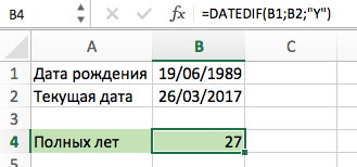
На примере выше, формула возвращает количество лет между двумя датами. Например, функция вернет значение “27” если вы захотите посчитать количество полных лет между двумя датами 19 июня 1989 года и 26 марта 2017 года. Система подсчитывает количество полных лет и игнорирует количество месяцев и дней между датами.
Разница дат в полных месяцах
Чтобы определить количество полных месяцев, которое прошло с одной даты до другой, необходимо воспользоваться такой же самой формулой, которая была приведена выше, только третий аргумент должен содержать аргумент m.
То есть, формула следующая.
=РАЗНДАТ(A2;B2;”m”)
Эта формула также может давать несколько неточные данные. Поэтому всегда нужно перепроверять значения самостоятельно.
Разница в днях без учета лет
Эта формула также может использоваться для определения количества дней между двумя датами, но при этом не учитывать количество лет, которое прошло между этими двумя временными точками. Эта возможность есть, но пользоваться ею настоятельно не рекомендуется, потому что искажений в этом случае может быть еще больше.
1
Эта формула вернет правильный результат только тогда, когда в компьютере показано правильное время. Конечно, в большинстве современных операционных системах дата и время определяется автоматически, но иногда случаются сбои. Поэтому перед тем, как подсчитывать разницу в днях без учета лет, нужно убедиться, что на компьютере установлена правильная дата и время. Особенно если электронная таблица пересылалась другому человеку.
Количество рабочих дней между двумя датами
Здесь ситуация чуть сложнее. Необходимо не учитывать субботы с воскресеньями и праздники. Для такого расчета лучше воспользоваться функцией ЧИСТРАБДНИ (NETWORKDAYS) из категории Дата и время. В качестве аргументов этой функции необходимо указать начальную и конечную даты и ячейки с датами выходных (государственных праздников, больничных дней, отпусков, отгулов и т.д.):

Примечание: Эта функция появилась в стандартном наборе функций Excel начиная с 2007 версии. В более древних версиях сначала необходимо подключить надстройку Пакета анализа. Для этого идем в меню Сервис — Надстройки (Tools — Add-Ins) и ставим галочку напротив Пакет анализа (Analisys Toolpak). После этого в Мастере функций в категории Дата и время появится необходимая нам функция ЧИСТРАБДНИ (NETWORKDAYS).
Сдвиг даты на заданное количество дней
Поскольку одни сутки в системе отсчета даты Excel принимаются за единицу (см.выше), то для вычисления даты, отстоящей от заданной на, допустим, 20 дней, достаточно прибавить к дате это число.
Сдвиг даты на заданное количество рабочих дней
Эту операцию осуществляет функция РАБДЕНЬ (WORKDAY). Она позволяет вычислить дату, отстоящую вперед или назад относительно начальной даты на нужное количество рабочих дней (с учетом выходных суббот и воскресений и государственных праздинков). Использование этой функции полностью аналогично применению функции ЧИСТРАБДНИ(NETWORKDAYS) описанной выше.
Вычисление дня недели
Вас не в понедельник родили? Нет? Уверены? Можно легко проверить при помощи функции ДЕНЬНЕД (WEEKDAY) из категории Дата и время.

Первый аргумент этой функции — ячейка с датой, второй — тип отсчета дней недели (самый удобный — 2).
Вычисление временных интервалов
Поскольку время в Excel, как было сказано выше, такое же число, как дата, но только дробная его часть, то с временем также возможны любые математические операции, как и с датой — сложение, вычитание и т.д.
Нюанс здесь только один. Если при сложении нескольких временных интервалов сумма получилась больше 24 часов, то Excel обнулит ее и начнет суммировать опять с нуля. Чтобы этого не происходило, нужно применить к итоговой ячейке формат 37:30:55:

Еще раз о кривизне РАЗНДАТ()
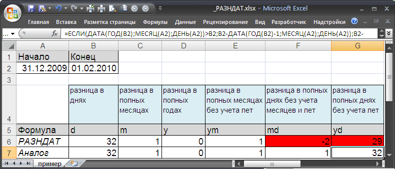
Найдем разницу дат 16.03.2015 и 30.01.15. Функция РАЗНДАТ() с параметрами md и ym подсчитает, что разница составляет 1 месяц и 14 дней. Так ли это на самом деле?
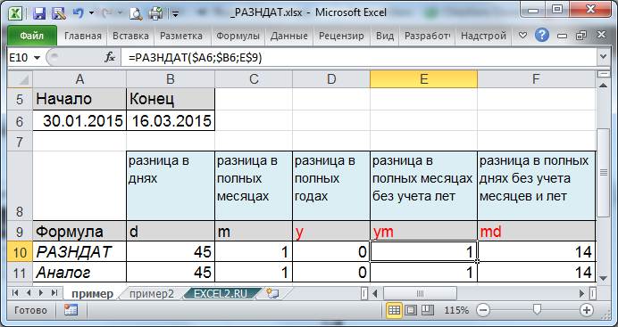
Имея формулу, эквивалентную РАЗНДАТ() , можно понять ход вычисления. Очевидно, что в нашем случае количество полных месяцев между датами = 1, т.е. весь февраль. Для вычисления дней, функция находит количество дней в предыдущем месяце относительно конечной даты, т.е. 28 (конечная дата принадлежит марту, предыдущий месяц — февраль, а в 2015г. в феврале было 28 дней). После этого отнимает день начала и прибавляет день конечной даты = ДЕНЬ(КОНМЕСЯЦА(ДАТАМЕС(B6;-1);0))-ДЕНЬ(A6)+ДЕНЬ(B6) , т.е. 28-30+16=14. На наш взгляд, между датами все же 1 полный месяц и все дни марта, т.е 16 дней, а не 14! Эта ошибка проявляется, когда в предыдущем месяце относительно конечной даты, дней меньше, чем дней начальной даты.
Формула возвращает разницу дат между сегодняшней и установленной планом в днях. Для решения данной задачи используется функция РАЗНДАТ в Excel: где найти эту формулу?
Данную функцию вы не найдете в мастере функций и даже на панели «ФОРМУЛЫ». Ее всегда нужно вводить вручную. Первым аргументом функции всегда должна быть новейшая дата, а вторым всегда – старшая дата. Третий аргумент функции определяет единицу измерения количества, которое возвращает функция =РАЗНДАТ(). В данном случае это символ «d» – дней. Это значит, что функция возвращает количество дней. Дальше следует оператор <7. То есть формула проверяет, если функция возвращает число меньше чем 7, то формула возвращает значение ИСТИНА и к текущей ячейке применяется условное форматирование. Ссылки на ячейки в первом аргумент абсолютная (значение неизменяемое), а во втором аргументе – относительная, так как проверятся будут несколько ячеек в столбце C.
При необходимости можно к данному диапазону добавить новое правило условного форматирования, которое будет предупреждать нас об окончании сроков за 2 недели.
Цвет форматирования для второго правила можно задать желтый. К одному и тому же диапазону должно быть применено 2 правила условного форматирования. Чтобы проверить выберите инструмент: «ГЛАВНАЯ»-«Стили»-«Условное форматирование»-«Управление правилами». Так как у нас сначала выполняется верхнее правило следует изменить их порядок в появившемся окне: «Диспетчер правил условного форматирования». Иначе все выделенные задачи будут иметь желтую заливку ячеек.
Полезный совет! Если к одному и тому же диапазону присвоено много правил – соблюдайте иерархию приоритетов порядка их выполнения в диспетчере управления правилами. Чем выше правило, тем выше его приоритет выполнения по отношению к другим расположенных ниже под ним.
Источники
- https://excelhack.ru/funkciya-datedif-razndat-v-excel/
- https://office-guru.ru/excel/data-vremja/kak-v-excel-sravnit-2-daty-mezhdu-soboj-prostaya-instrukciya.html
- http://word-office.ru/kak-sdelat-sravnenie-dat-v-excel.html
- https://excelka.ru/voprosy/kak-v-excel-sravnit-dve-daty.html
- https://exceltable.com/formatirovanie/raznica-mejdu-datami
The DATEDIF function is categorized as a DATE/TIME function in Excel. The function name almost gives away its purpose. It calculates the difference (DIF) between two given dates (DATE). This function is particularly useful for financial analysts. For instance, when they need to calculate the holding period in terms of days, months, or years.
DATEDIF is an undocumented function, this means you would not find this function in the formula tab. In addition to this, Excel will also not help you with IntelliSense (the suggestions Excel provides while you type function syntax) while writing the DATEDIF function, but it works well when configured correctly.

Note: Please note that DATEDIF Function in Excel is totally different from the DATEDIFF (notice the extra ‘F’) function in VBA.
Syntax
Learning the syntax of the DATEDIF function is crucial since Excel won’t help you with IntelliSense. The syntax is as follows:
=DATEDIF(start_date, end_date, unit)
Arguments:
‘start_date‘ – This is a required argument where you will need to insert the starting date.
‘end_date‘ – This is a required argument where you will need to insert the ending date.
‘unit‘ – This argument is supplied as a text string and represents the units in which we want the formula to compute the difference. You may use the table given below for appropriate codes required for the desired results.
Codes for Unit Argument
| UNIT | DESCRIPTION |
|---|---|
| «Y» | Returns difference as complete years. |
| «M» | Returns the difference as complete months. |
| «D» | Returns the difference in days. |
| «MD» | Returns the difference in days, ignoring months and years. |
| «YM» | Returns the difference in months, ignoring years. |
| «YD» | Returns the difference in days, ignoring years. |
Important Characteristics of the DATEDIF function
- The DATEDIF function is an undocumented compatibility function inherited from Lotus 1-2-3. When you start typing the DATEDIF function, Excel won’t show any suggestions as it does for other functions.
- The DATEDIF function accepts inputs in the form of a text string, serial numbers, or relayed output from other Excel functions.
- If the date entered as start_date occurs after the end_date, the function will return a #NUM error. If either of the arguments is supplied with a date that Excel doesn’t recognize, the function will return a #VALUE error.
Examples
Let’s try to see some examples of the DATEDIF function.
Example 1 – Plain Vanilla Formula for the DATEDIF Function
Let’s just test the waters first to see how the DATEDIF function works in its simplest form. We have two dates in cells A2 and B2, and we’ll compute the difference between them using the following formula:
=DATEDIF(A2, B2, "d")

The formula sets the unit to «d» which means the final output will be in terms of complete days. The function will return the difference in days between the two dates supplied in the first two arguments. In our example, the difference comes to 1985 days.
Note that this computation could have been made without using the DATEDIF function. Excel stores dates as serial numbers, and subtracting one serial number from the other would effectively return the difference in the number of days.
Example 2 – Count Difference in Days (All Variations)
Alright Excel ninjas, we already discussed that there are multiple ways to obtain output from the DATEDIF function. We’ll now talk about the options available for obtaining the difference in terms of days.
We saw the output that «d» gives us. Let’s also take a quick look at what «yd» and «md» return when used in the DATEDIF function.
=DATEDIF(A2, B2, "d") //difference in days
=DATEDIF(A3, B3, "yd") //difference in days, year component is ignored
=DATEDIF(A4, B4, "md") //difference in days, ignores both month and year components

When we use «yd» in the unit argument, the difference is calculated in terms of days, but the year component is ignored. In effect, the difference will be calculated as if the start and end date occurred in the same year. Therefore, the difference, in this case, reduces to 158 from 1985.
When we use «md» in the unit argument, the difference is calculated in days, but this time around, the function will ignore both month and year components. In this case, the difference is calculated as though both dates occur in the same month and same year. Therefore, the difference further reduces to 5 from 158.
Example 2 – Count Difference in Months (All Variations)
Crack your knuckles because we have a few more ways to calculate the difference between two dates. This time around, we’ll calculate the difference in terms of months.
=DATEDIF(A2, B2, "m") //difference in months
=DATEDIF(A3, B3, "ym") //difference in months, year component is ignored

When we use «m» in the unit argument, Excel computes the difference in months as any person would. Every 30/31 days add one month to the tally. In our example, the formula returns 65 months.
However, when we use «ym» in the unit argument, the output changes to 5. This is because now, Excel ignores the year component and only computes the difference in number of months. It’s the same as saying that Excel assumes that both the start and end dates occur in the same year. Therefore, the output reduces to 5.
Cool, right?
We’re not done, though…
Example 3 – Count Difference in Years
The inception that the unit argument has created ends here. There is only one way to calculate the difference in the number of years, like so:
=DATEDIF(A2, B2, "y") //difference in years

It’s rather simple. Excel just gives us the complete difference between the two years. In our example, the difference is 5.
However, note that the difference isn’t exactly 5. Since the day and month for both dates are different, there has to be some fractional year that the DATEDIF function ignored. If you want a precise difference, you could use the YEARFRAC function like so:
=YEARFRAC(A2, B2) //exact difference in terms of years

The YEARFRAC function will give you an exact difference, which in this case, is 5.43 years.
Example 4 – Get Years, Months, and Days Between Two Dates
It’s time to raise our ambitions and accomplish a little more with this nifty Excel function. This time around, we’re going to calculate the difference in terms of years, months, and days together using the DATEDIF function.
We can do this with the following formula:
=DATEDIF(A2, B2, "y")&" year(s), "& DATEDIF(A2, B2, "ym")& " month(s), " & DATEDIF(A2, B2, "md")&" day(s)"

Don’t be overwhelmed by the size of the formula, we’ll punch it flat in just a moment.
There are three formulas in here, joined together as one using the concatenation operator. We’ve already discussed those individual formulas in the previous examples, so let’s get to the logic of how this formula comes together.
The first DATEDIF calculates the difference in years. Plain and simple.
The second DATEDIF calculates the difference in months but ignores the years. This works out because we’ve already calculated the difference in years using the first DATEDIF.
The third DATEDIF calculates the difference in days but ignores both months and years. Again, this works since both the difference in months and years has already been calculated using the previous two DATEDIFs.
There’s one more component in the formula—the text strings. They are just concatenated with the DATEDIF function’s output for better presentation and don’t contribute to any computations in the formula.
This is how Excel calculated the final output of 5 years, 5 months, 5 days.
Easy-peasy, isn’t it?
Example 5 – Calculating Age from Date of Birth
Let’s draw some inspiration from the previous formula and use it for a noble purpose—calculating the spouse’s age. I got into a friendly argument with my spouse and she begs to differ on her exact age. We decided to get creative and pulled up a spreadsheet.
Calculating age in Excel is pretty simple, we just modified the previous formula slightly to get this done:
=DATEDIF(A2, TODAY(), "y")&" year(s), "& DATEDIF(A2, TODAY(),"ym")& " month(s), " & DATEDIF(A2, TODAY(), "md")&" day(s)"

A light bulb probably already went off as you skimmed through this formula, but I’ll still point it out—the only difference here is the use of TODAY function.
The TODAY function works as our end_date argument since we want to compute the difference from a certain date (the DOB) right up to today.
Cell A2, of course, contains the Date of Birth that will work as our starting point. Other than that, the formula uses the same logic as it did in the previous example.
The output, therefore, is 26 years, 3 months, 10 days. I obviously didn’t use her actual DOB since I don’t like sleeping on the couch.
Alright, with this, we’ve covered the DATEDIF function inside out. Consider yourself an expert on the DATEDIF function once you’ve practiced these formulas thoroughly. However, I strongly recommend against using your spouse’s DOB when you practice. While you keep yourself busy with the DATEDIF function, we’ll have another Excel function loaded up, ready to fire away!