
Excel for Microsoft 365 for Mac Excel 2021 for Mac Excel 2019 for Mac Excel 2016 for Mac Excel for Mac 2011 More…Less
You can use number formats to change the appearance of numbers, including dates and times, without changing the actual number. The number format does not affect the cell value that Excel uses to perform calculations. The actual value is displayed in the formula bar.
Excel provides several built-in number formats. You can use these built-in formats as is, or you can use them as a basis for creating your own custom number formats. When you create custom number formats, you can specify up to four sections of format code. These sections of code define the formats for positive numbers, negative numbers, zero values, and text, in that order. The sections of code must be separated by semicolons (;).
The following example shows the four types of format code sections.

 Format for positive numbers
 Format for negative numbers
 Format for zeros
 Format for text
If you specify only one section of format code, the code in that section is used for all numbers. If you specify two sections of format code, the first section of code is used for positive numbers and zeros, and the second section of code is used for negative numbers. When you skip code sections in your number format, you must include a semicolon for each of the missing sections of code. You can use the ampersand (&) text operator to join, or concatenate, two values.
Create a custom format code
-
On the Home tab, click Number Format
 , and then click More Number Formats.
 -
In the Format Cells dialog box, in the Category box, click Custom.
-
In the Type list, select the number format that you want to customize.
The number format that you select appears in the Type box at the top of the list.
-
In the Type box, make the necessary changes to the selected number format.
 , and then click More Number Formats.
Format code guidelines
To display both text and numbers in a cell, enclose the text characters in double quotation marks (» «) or precede a single character with a backslash (). Include the characters in the appropriate section of the format codes. For example, you could type the format $0.00″ Surplus»;$–0.00″ Shortage» to display a positive amount as «$125.74 Surplus» and a negative amount as «$–125.74 Shortage.»
You don’t have to use quotation marks to display the characters listed in the following table:
|
Character |
Name |
|
$ |
Dollar sign |
|
+ |
Plus sign |
|
— |
Minus sign |
|
/ |
Forward slash |
|
( |
Left parenthesis |
|
) |
Right parenthesis |
|
: |
Colon |
|
! |
Exclamation point |
|
^ |
Circumflex accent (caret) |
|
& |
Ampersand |
|
‘ |
Apostrophe |
|
~ |
Tilde |
|
{ |
Left curly bracket |
|
} |
Right curly bracket |
|
< |
Less than sign |
|
> |
Greater than sign |
|
= |
Equal sign |
|
Space character |
To create a number format that includes text that is typed in a cell, insert an «at» sign (@) in the text section of the number format code section at the point where you want the typed text to be displayed in the cell. If the @ character is not included in the text section of the number format, any text that you type in the cell is not displayed; only numbers are displayed. You can also create a number format that combines specific text characters with the text that is typed in the cell. To do this, enter the specific text characters that you want before the @ character, after the @ character, or both. Then, enclose the text characters that you entered in double quotation marks (» «). For example, to include text before the text that’s typed in the cell, enter «gross receipts for «@ in the text section of the number format code.
To create a space that is the width of a character in a number format, insert an underscore (_) followed by the character. For example, if you want positive numbers to line up correctly with negative numbers that are enclosed in parentheses, insert an underscore at the end of the positive number format followed by a right parenthesis character.
To repeat a character in the number format so that the width of the number fills the column, precede the character with an asterisk (*) in the format code. For example, you can type 0*– to include enough dashes after a number to fill the cell, or you can type *0 before any format to include leading zeros.
You can use number format codes to control the display of digits before and after the decimal place. Use the number sign (#) if you want to display only the significant digits in a number. This sign does not allow the display non-significant zeros. Use the numerical character for zero (0) if you want to display non-significant zeros when a number might have fewer digits than have been specified in the format code. Use a question mark (?) if you want to add spaces for non-significant zeros on either side of the decimal point so that the decimal points align when they are formatted with a fixed-width font, such as Courier New. You can also use the question mark (?) to display fractions that have varying numbers of digits in the numerator and denominator.
If a number has more digits to the left of the decimal point than there are placeholders in the format code, the extra digits are displayed in the cell. However, if a number has more digits to the right of the decimal point than there are placeholders in the format code, the number is rounded off to the same number of decimal places as there are placeholders. If the format code contains only number signs (#) to the left of the decimal point, numbers with a value of less than 1 begin with the decimal point, not with a zero followed by a decimal point.
|
To display |
As |
Use this code |
|
1234.59 |
1234.6 |
####.# |
|
8.9 |
8.900 |
#.000 |
|
.631 |
0.6 |
0.# |
|
12 1234.568 |
12.0 1234.57 |
#.0# |
|
Number: 44.398 102.65 2.8 |
Decimal points aligned: 44.398 102.65 2.8 |
???.??? |
|
Number: 5.25 5.3 |
Numerators of fractions aligned: 5 1/4 5 3/10 |
# ???/??? |
To display a comma as a thousands separator or to scale a number by a multiple of 1000, include a comma (,) in the code for the number format.
|
To display |
As |
Use this code |
|
12000 |
12,000 |
#,### |
|
12000 |
12 |
#, |
|
12200000 |
12.2 |
0.0,, |
To display leading and trailing zeros prior to or after a whole number, use the codes in the following table.
|
To display |
As |
Use this code |
|
12 123 |
00012 00123 |
00000 |
|
12 123 |
00012 000123 |
«000»# |
|
123 |
0123 |
«0»# |
To specify the color for a section in the format code, type the name of one of the following eight colors in the code and enclose the name in square brackets as shown. The color code must be the first item in the code section.
[Black] [Blue] [Cyan] [Green] [Magenta] [Red] [White] [Yellow]
To indicate that a number format will be applied only if the number meets a condition that you have specified, enclose the condition in square brackets. The condition consists of a comparison operator and a value. For example, the following number format will display numbers that are less than or equal to 100 in a red font and numbers that are greater than 100 in a blue font.
[Red][<=100];[Blue][>100]
To hide zeros or to hide all values in cells, create a custom format by using the codes below. The hidden values appear only in the formula bar. The values are not printed when you print your sheet. To display the hidden values again, change the format to the General number format or to an appropriate date or time format.
|
To hide |
Use this code |
|
Zero values |
0;–0;;@ |
|
All values |
;;; (three semicolons) |
Use the following keyboard shortcuts to enter the following currency symbols in the Type box.
|
To enter |
Press these keys |
|
¢ (cents) |
OPTION + 4 |
|
£ (pounds) |
OPTION + 3 |
|
¥ (yen) |
OPTION + Y |
|
€ (euro) |
OPTION + SHIFT + 2 |
The regional settings for currency determine the position of the currency symbol (that is, whether the symbol appears before or after the number and whether a space separates the symbol and the number). The regional settings also determine the decimal symbol and the thousands separator. You can control these settings by using the Mac OS X International system preferences.
To display numbers as a percentage of 100 — for example, to display .08 as 8% or 2.8 as 280% — include the percent sign (%) in the number format.
To display numbers in scientific notation, use one of the exponent codes in the number format code — for example, E–, E+, e–, or e+. If a number format code section contains a zero (0) or number sign (#) to the right of an exponent code, Excel displays the number in scientific notation and inserts an «E» or «e». The number of zeros or number signs to the right of a code determines the number of digits in the exponent. The codes «E–» or «e–» place a minus sign (-) by negative exponents. The codes «E+» or «e+» place a minus sign (-) by negative exponents and a plus sign (+) by positive exponents.
To format dates and times, use the following codes.
Important: If you use the «m» or «mm» code immediately after the «h» or «hh» code (for hours) or immediately before the «ss» code (for seconds), Excel displays minutes instead of the month.
|
To display |
As |
Use this code |
|
Years |
00-99 |
yy |
|
Years |
1900-9999 |
yyyy |
|
Months |
1-12 |
m |
|
Months |
01-12 |
mm |
|
Months |
Jan-Dec |
mmm |
|
Months |
January-December |
mmmm |
|
Months |
J-D |
mmmmm |
|
Days |
1-31 |
d |
|
Days |
01-31 |
dd |
|
Days |
Sun-Sat |
ddd |
|
Days |
Sunday-Saturday |
dddd |
|
Hours |
0-23 |
h |
|
Hours |
00-23 |
hh |
|
Minutes |
0-59 |
m |
|
Minutes |
00-59 |
mm |
|
Seconds |
0-59 |
s |
|
Seconds |
00-59 |
ss |
|
Time |
4 AM |
h AM/PM |
|
Time |
4:36 PM |
h:mm AM/PM |
|
Time |
4:36:03 PM |
h:mm:ss A/P |
|
Time |
4:36:03.75 PM |
h:mm:ss.00 |
|
Elapsed time (hours and minutes) |
1:02 |
[h]:mm |
|
Elapsed time (minutes and seconds) |
62:16 |
[mm]:ss |
|
Elapsed time (seconds and hundredths) |
3735.80 |
[ss].00 |
Note: If the format contains AM or PM, the hour is based on the 12-hour clock, where «AM» or «A» indicates times from midnight until noon and «PM» or «P» indicates times from noon until midnight. Otherwise, the hour is based on the 24-hour clock.
See also
Create and apply a custom number format
Display numbers as postal codes, Social Security numbers, or phone numbers
Display dates, times, currency, fractions, or percentages
Highlight patterns and trends with conditional formatting
Display or hide zero values
Need more help?
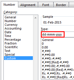
What is the Date Format in Excel?
In Excel, a date is displayed according to the format selected by the user. One can choose from the different formats available or create a customized format according to the requirement. The default date format is specified in the “Control Panel” of the system. However, it is possible to change these default settings.
For example, the date 01/01/2021 corresponds to the format dd/mm/yyyy. If the format is changed to d-mmm-yyyy, the date becomes 1-Jan-2021.
We can change the date format in Excel either from the “Number Format” of the “Home” tab or the “Format Cells” option of the context menu.
In Excel for Windows, 1900 is the default date system. Whereas, in Excel for Mac, 1904 is the default date system. Both these systems store the dates as consecutive numbers having a difference of 1. These numbers are known as serial values or serial numbers. The reason dates are stored as serial numbers is to facilitate calculations.
In the 1900 date system, the first date that Excel recognizes is January 1, 1900. This date is stored as the number 1 in Excel. Consequently, the number 2 represents January 2, 1900. The last date recognized by Excel is December 31, 9999. It is represented by the serial number 2958465. Date before 1900 or after 9999 is identified as a text value by Excel.
Dates are stored only as positive integers in the 1900 date system. However, to display negative numbers as negative dates, one needs to switch to the 1904 date system.
In the 1904 date system, 0 represents January 1, 1904, and -1 means January -2, 1904. The number 1 represents January 2, 1904. The last date recognized by Excel (in the 1904 date system) is December 31, 9999, represented by the serial number 2957003.
In this article, we follow the 1900 date system.
Table of contents
- What is theDate Format in Excel?
- Code of Date Format in Excel
- How to Change Date Format in Excel?
- Example #1–Apply Default Format of Long Date in Excel
- Example #2–Change the Date Excel Format Using “Custom” Option
- Example #3–Apply Different Types of Customized Date Formats in Excel
- Example #4–Convert Text Values Representing Dates to Actual Dates
- Example #5–Change the Date Format Using “Find and Replace” Box
- Frequently Asked Questions
- Recommended Articles
Code of Date Format in Excel
A code (like dd-mm-yyyy) is a representation of a day (d), month (m), and year (y). We can change the appearance of the date by changing the specified code.
The different codes, their explanation, and output (for days, months, and years) have been presented in the following images.
Notations for a Day

Notations for a Month

Notations for a Year
How to Change Date Format in Excel?
Here we look at some of the date format examples in Excel and how to change them.
Example #1–Apply Default Format of Long Date in Excel
The following image shows a number in cell A1. We want to know the date represented by this number. The output should be in the long date format of Excel.
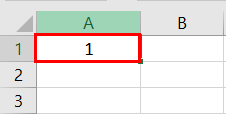
The steps to know the date represented by the number in cell A1 are listed as follows:
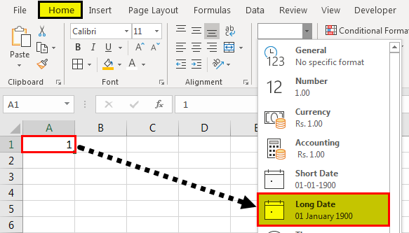
- We must first select cell A1. Then, from the “Home” tab, click the “Number Format” drop-down appearing in the “Number” section. Next, select “Long Date,” shown in the following image.

- The output is shown in the following image. The long date format displayed is dd mmmm yyyy. Hence, the number 1 represents the date 01 January 1900 in the long date format.
Note: The short and long dates appear as set in the “Control Panel.” Click “Clock, Language, and Region” in the “Control Panel” to change these default date formats. After that, click “Change date, time, or number formats.” Make the desired changes and click “OK.”
Likewise, had there been 2 in cell A1, the long date format would have been 02 January 1900. The number 3 would have been displayed as 03 January 1900 in the long date format.
Note: To switch to the 1904 date system, we must select “Advanced” from the “Options” of the “File” tab. Under “When calculating this workbook,” select “use 1904 date system” and click “OK.”

You can download this Change Date Format Excel Template here – Change Date Format Excel Template
Example #2–Change the Date Excel Format Using “Custom” Option
The following image shows some dates in the range A1:A6. These dates are in the format dd-mm-yyyy. We want to change their format to dd-mmmm-yyyy.
For instance, the date in cell A1 should appear as 25-February-2018. We may use the “Custom” option of the “Format Cells” dialog box.

The steps to change the date format in Excel are listed as follows:
Step 1: We need to select all the dates of the range A1:A6. The same is shown in the following image.
Step 2: We must right-click the selection and choose “Format Cells” from the context menu. Alternatively, we may also press the keys “Ctrl+1” together.
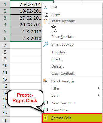
Step 3: The “Format Cells” window opens, as shown in the following image.
Note: The default short date and long date formats are marked with an asterisk (*) in the box under “type.” The short date is 3/14/2012 (m/dd/yyyy), and the long date is Wednesday, March 14, 2012 (dddd, mmmm dd, yyyy).
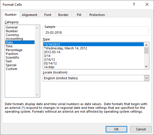
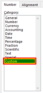
Step 4: From the “Number” tab, we need to select “Custom” under “Category.” The categories are shown on the left side of the “Format Cells” window.
Step 5: Under “Type,” we must insert the required date format. Either type the format (dd-mmmm-yyyy) or select it from the various options displayed in the box below “Type.”
Once the format has been entered, check the preview of the first date (of the range A1:A6) under “Sample.” The same is shown in the following image. Click “OK” in the “Format Cells” window if the date preview looks good.
Note 1: The date under “Sample” is displayed according to the format specified under “Type.”
Note 2: While creating custom date formats, we can use a forward slash (/), hyphen (-), comma (,), space ( ), etc.

Step 6: The output is shown in the following image. All dates of the range A1:A6 have been converted to the format dd-mmmm-yyyy. However, the Excel formula bar can still see the default date format. This default format corresponds with the short date set in the “Control Panel.”

Example #3–Apply Different Types of Customized Date Formats in Excel
The next image shows certain dates in the range A1:A6. At present, the date format is dd-mm-yyyy.
We want to apply four different formats to these dates. For using each format, the common steps to be performed are given as follows:
- First, we must select the range A1:A6.
- Then, right-click the selection and choose “Format Cells.”
- After that, from the “Number” tab, select “Custom” under “Category.”
Further, under each format, the additional steps to be performed followed by two images are given.

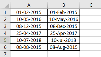
Format 1: dd-mmm-yyyy
- In the “Custom” option of the “Number” tab, select the format “dd-mmm-yyyy” under “Type.”
- Click “Ok.”

The output is given in the following image. All dates are displayed according to the format dd-mmm-yyyy. The hyphen is the separator between the day, month, and year in this format.

Format 2: dd mmm yyyy
- We must select the format “dd mmm yyyy” under “Type” of the “custom” option.
- Click “Ok.”

The output is given in the following image. All dates are converted to the format dd mmm yyyy. The space is the only separator between the day, month, and year in this format.

Format 3: ddd mmm yyyy
- In the “Custom” option, select the format “ddd mmm yyyy” under “Type.”
- Click “Ok.”

The output is given in the following image. The dates are shown in the format ddd mmm yyyy. The day and the month are displayed in their short notations in this format.

Format 4: dddd mmmm yyyy
- From the “Custom” option of the “Number” tab, select “dddd mmmm yyyy” under “Type.”
- Click “Ok.”

The output is given in the following image. All dates have been converted to the format dddd mmmm yyyy. The date, month, and year are displayed in their respective full forms in this format.

It must be observed that the date format changes as per the style set by the user. Therefore, the user can select a date format according to their convenience.
Example #4–Convert Text Values Representing Dates to Actual Dates
The following image shows a list of dates in the range A1:A6. At present, these dates are appearing as text values. We want to convert these text values to dates having the format dd-mmm-yyyy.

The steps to convert text values to dates having the given format are listed as follows:
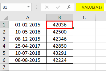
Step 1: First, enter the following formula in cell B1.
“=VALUE(A1)”
Then, press the “Enter” key.
Note 1: The VALUE functionIn Excel, the value function returns the value of a text representing a number. So, if we have a text with the value $5, we can use the value formula to get 5 as a result, so this function gives us the numerical value represented by a text.read more returns the numeric form of a text string that represents a number. In other words, it converts a number looking like the text into an actual number.
Note 2: Instead of the VALUE function, one can also use the DATEVALUE functionThe DATEVALUE function in Excel shows any given date in absolute format. This function takes an argument in the form of date text normally not represented by Excel as a date and converts it into a format that Excel can recognize as a date.read more of Excel. The latter converts a date stored as text to a serial number. This serial number is recognized as a date by Excel.
Step 2: We must select cell B1 and drag the fill handle until cell B6. The output is shown in the following image. All text values (A1:A6) have been converted to numbers (in the range B1:B6).
Ideally, the text string in Excel is left-aligned while the number string is right-aligned. However, we have centrally aligned both the ranges (A1:A6 and B1:B6).
Note: When text strings representing dates have been converted to serial values (or dates), we can use them for performing different calculations like addition, subtraction, and so on.
Step 3: To view the obtained serial numbers (in column B) as dates, apply the required format. We must select the range B1:B6, right-click and choose “Format Cells.”
In the “Number” tab, select the option “Custom.” Then, under “Type,” enter or choose the format “dd-mmm-yyyy.” The same is shown in the following image.
If the sample date looks alright, click “OK.”
Step 4: The output is shown in the following image. Hence, all text values (of column A) have been converted to valid dates (in column B) having the format dd-mmm-yyyy.
Note: To ensure that a value is recognized as a date by Excel, check for the following signs:
- The dates are right-aligned as they are numerical values.
- If two or more dates are selected, the status bar (at the bottom of the worksheet) shows the count, average, numerical count, and sum. In addition, it may display one or more options according to the Excel version.
If a value is a text string, it would be left-aligned, and the status bar will show only the count.
Often, the Excel date format needs to be changed (from text to dates) when data is downloaded (or copied and pasted) from the web. That is because, in such instances, the dates may not be displayed as numbers.
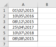
Example #5–Change the Date Format Using “Find and Replace” Box
The following image shows some text values representing dates in the range A1:A6. The days, months, and numbers have been separated with a backslash. That is because we want to perform the following tasks:
- Replace all the backslashes () with forwarding slashes (/) by using the “Find and Replace” dialog box.
- Convert text values representing dates to actual dates.
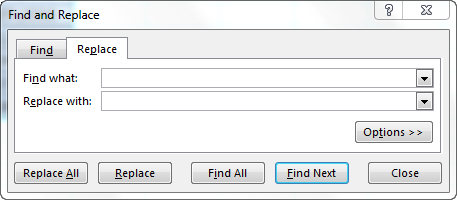
The steps to perform the given tasks are listed as follows:
Step 1: We must press the keys “Ctrl+H” together. Then, the “find and replace” dialog box opens, as shown in the following image.
Step 2: Type a backslash in the “Find what” box (). In the “Replace with” box, type a forward slash (/).
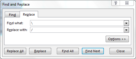
Step 3: Next, we must click “Replace All.” Excel shows a message stating the number of replacements it has made. Click “OK” to proceed. The final output is shown in the following image.
Hence, all backslashes have been replaced with forwarding slashes. With this replacement, the text values representing dates have automatically been converted to actual dates by Excel.
Since column A was aligned centrally from the beginning, this alignment is retained even after the values are converted to dates.

Frequently Asked Questions
1. How can the date format in Excel be changed?
The steps to change the date format in Excel are listed as follows:
The steps to change the date format in Excel are listed as follows:
a. Select the cell containing the date. If the date format of a range needs to be changed, select the entire range.
b. Right-click the selection and choose “Format Cells” from the context menu. Alternatively, press the keys “Ctrl+1” together.
c. IIn the “Number” tab, select the option “Date.” Next, select the required date format under “Type.”
d. Check the preview (of the first date of the selected range) under “Sample.” If the preview is good, click “OK.”
The date format of the selected cell or cells (selected in step a) is changed.
Note 1: The required date format may not be available under the “Date” option’s “Type.” If it is not available, select “Custom” as the “category” from the “Number” tab. Then, type the required date format under “Type” and click “OK.”
Note 2: If the selected cell (selected in step a) contains a text string representing a date, convert this string to date first. Then change the format to the desired date format.
2. How to change the date format permanently in Excel?
To change a date format permanently, one needs to make changes to the date formats of the “Control Panel.” That is because the short and long date formats of Excel reflect the date settings of the “Control Panel.”
The steps to change the date settings of the “Control Panel” are listed as follows:
We must open the “Control Panel” first from the “Start” menu.
b. In the “Clock, Language, and Region” category, click “Change date, time, or number format.” It is available under the “Region and Language” option.
c. The “Region and Language” or “Region” dialog box opens. Under “Format,” we must select the region.
d. Enter the required short and long date formats under “Date and Time Formats.” To enter customized short and long date formats, click “Additional Settings.” The “Customize Format” dialog box opens. Make the changes in the “Date” tab and click “OK.”
e. Check the preview under “Examples” at the bottom of the “Region and Language” box. If the preview is alright, click “OK.”
The default date settings have been changed. Now, we should enter a date in any format in Excel. Then select the short or the long date format from the “Number Format” (in the “Number” section) of the “Home” tab.
The dates will appear in the format set in the “Control Panel.” So, the user need not change the format of each date manually.
3. How to change a date to a text string in Excel?
Let us change the date 22/1/2019 in cell A1 to a text string in Excel. The text string should be in the format yyyy-mm-dd.
The steps to change a date to a text string are listed as follows:
a. First, we must enter the formula =TEXT(A1, “yyyy-mm-dd”) in cell B1.
b. Then, press the “Enter” key.
The date in cell A1 (22/1/2019) is converted to 2019-01-22 in cell B1. We must note that the date in cell A1 is right-aligned, being a number. In contrast, the text in cell B1 is left-aligned.
Note: The TEXT function helps convert numbers to text strings. It is used to display values in a specific format. The syntax is TEXT(value,format_text). “Value” is the number to be converted to text. “Format_text” is the format in which the number should be displayed.
Recommended Articles
This article has been a guide to the Date Format in Excel. We discuss changing and customizing date formats in Excel, practical examples, and a downloadable Excel template. You may also look at these useful functions in Excel: –
- Concatenate Columns in Excel
- Convert Date to Text in Excel
- Insert Date in Excel
- Concatenate Date in Excel
 Please Note:
This article is written for users of the following Microsoft Excel versions: 2007, 2010, 2013, 2016, 2019, and Excel in Microsoft 365. If you are using an earlier version (Excel 2003 or earlier), this tip may not work for you. For a version of this tip written specifically for earlier versions of Excel, click here: Understanding Date and Time Formatting Codes.
![]()
Written by Allen Wyatt (last updated October 12, 2019)
This tip applies to Excel 2007, 2010, 2013, 2016, 2019, and Excel in Microsoft 365
In Excel, dates and times are stored internally as numbers. These are only converted to legible dates and times when you format the cell using a date or time format. You can use one of Excel’s pre-defined date and time formats or you can create your own custom format.
Regardless of which approach you take, you use the Number tab of the Format Cells dialog box (display the Home tab of the ribbon, click the small icon at the bottom-right of the Number group, then make sure the Number tab is displayed.) The Date, Time, and Custom options all appear at the right of the dialog box. (See Figure 1.)
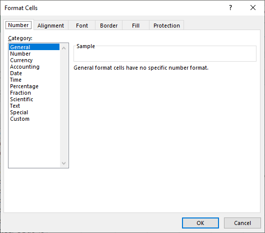
Figure 1. The Number tab of the Format Cells dialog box.
If you create a custom format for your dates and times, you need to become conversant in the codes you can use to define those formats. The following table lists the formatting codes that are specific to dates and times. You use these codes when you are creating a custom display format (display the Home tab of the ribbon, click the small icon at the bottom-right of the Number group, then choose Custom in the Category list).
| Symbol | Meaning | |
|---|---|---|
| m | Displays the month or minutes as a number without a leading 0 | |
| mm | Displays the month or minutes as a number with a leading 0 | |
| mmm | Displays the month as abbreviated text (Jan, Feb, Mar, and so on) | |
| mmmm | Displays the month as text (January, February, March, and so on) | |
| d | Displays the day of the month as a number without a leading 0 | |
| dd | Displays the day of the month as a number with a leading 0 | |
| ddd | Displays the day of the week as abbreviated text (Sun, Mon, Tue, and so on) | |
| dddd | Displays the day of the week as text (Sunday, Monday, Tuesday, and so on) | |
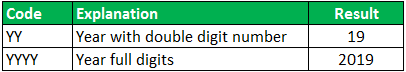
| yy | Displays the year with two digits | |
| yyyy | Displays the year with four digits | |
| h | Displays the hour without a leading 0 | |
| hh | Displays the hour with a leading 0 | |
| s | Displays the seconds without a leading 0 | |
| ss | Displays the seconds with a leading 0 | |
| [ ] | When surrounding hours, minutes, or seconds place holders, displays hours greater than 24 or minutes and seconds greater than 60 | |
| AM am PM pm A a P p | Uses a 12-hour clock, displaying AM or PM as specified | |
| Forces display of the following character | ||
| . (period) | The decimal point. | |
| «text» | Displays the text within the quotes. |
To understand better the effect of the date and time codes, take a look at the following information, which shows several common date and time formats and how they affect numbers.
| Category | Format | Value | Displayed As | |||
|---|---|---|---|---|---|---|
| Date | m/d/yy | 34369 | 2/4/94 | |||
| d-mmm-yy | 34409 | 16-Mar-94 | ||||
| Time | h:mm AM/PM | 0.654166667 | 3:42 PM | |||
| [h]:mm:ss | 2.592673611 | 62:13:27 |
Notice that the numbers shown in the value column of these examples are the internal values stored by Excel for dates and times.
ExcelTips is your source for cost-effective Microsoft Excel training.
This tip (8319) applies to Microsoft Excel 2007, 2010, 2013, 2016, 2019, and Excel in Microsoft 365. You can find a version of this tip for the older menu interface of Excel here: Understanding Date and Time Formatting Codes.
Author Bio
With more than 50 non-fiction books and numerous magazine articles to his credit, Allen Wyatt is an internationally recognized author. He is president of Sharon Parq Associates, a computer and publishing services company. Learn more about Allen…
MORE FROM ALLEN
Turning Off AutoComplete for Dates
The AutoComplete feature can be helpful. However, there are times when the suggestions Word makes aren’t what you want. …
Discover More
Automatically Protecting After Input
Do you want user-entered data to be immediately protected so that it cannot be changed? This can be done relatively …
Discover More
Formatting Lots of Tables
Do you need a quick way to format your tables? Believe it or not, there are several tools you can use from Word’s arsenal …
Discover More
What is a date in Excel?
A date is a number! And like any number (currency, percentage, decimal, …), you can customize your date format 👍
Dates are whole numbers
Usually, when you insert a date in a cell it is displayed in the format dd/mm/yyyy or mm/dd/yyyy.
Let’s say you have the date 01/01/2016 in a cell. If you change the cell’s format to Standard, the cell displays 42370 😕🤔

Explanation of the numbering
In Excel, a date is the number of days since 01/01/1900 (the first date in Excel).
So 42370 is the number of days between 01/01/1900 and 01/01/2016.
Date format
Dates can be displayed in different ways using the following 2 options (available in the Number Format dropdown in the main menu):
- Short Date
- Long Date

How to customize a date?
To customize a date:
- Open the dialog box Custom Number (with the shortcut Ctrl + 1 or by clicking on the menu More number formats at the bottom of the number format dropdown)

- In this dialog box, you select ‘Custom‘ in the Category list and write the date format code in ‘Type‘.

To format a date, you just write the parameter d, m or y a different number of times. For example,
- dd/mm/yyyy will display 01/01/2016
- dd mmm yyyy => 01 Jan 2016
- mmmm yyyy => January 2016
- dddd dd => Friday 01
In function of your language , the letter could be different:
- t for «tag» (day) in German
- j for «jour» (day) in French
- a for «año» (year) in Spanish
Don’t write text in your cell !!!
With dates, one of the most common mistakes is to write text inside the format code (1 January 2016 for example). Never do this in Excel ⛔⛔⛔
If you do this, the contents of the cell will be Text and not a number
- In Excel, text is always displayed on the left of a cell.
- A number or a date is displayed on the right.

If you want to display the month in letters, just change the month format of your date.
Different examples of custom date
The following document shows you the same date but in different formats. The code for each date is in column A.

Different writing of dates according to the format code
In the following document, you can see the impact of each format on the same date.

Introduction
Number formats control how numbers are displayed in Excel. The key benefit of number formats is that they change how a number looks without changing any data. They are a great way to save time in Excel because they perform a huge amount of formatting automatically. As a bonus, they make worksheets look more consistent and professional.
Video: What is a number format
What can you do with custom number formats?
Custom number formats can control the display of numbers, dates, times, fractions, percentages, and other numeric values. Using custom formats, you can do things like format dates to show month names only, format large numbers in millions or thousands, and display negative numbers in red.

Where can you use custom number formats?
Many areas in Excel support number formats. You can use them in tables, charts, pivot tables, formulas, and directly on the worksheet.
- Worksheet — format cells dialog
- Pivot Tables — via value field settings
- Charts — data labels and axis options
- Formulas — via the TEXT function
What is a number format?
A number format is a special code to control how a value is displayed in Excel. For example, the table below shows 7 different number formats applied to the same date, January 1, 2019:
| Input | Code | Result |
|---|---|---|
| 1-Jan-2019 | yyyy | 2019 |
| 1-Jan-2019 | yy | 19 |
| 1-Jan-2019 | mmm | Jan |
| 1-Jan-2019 | mmmm | January |
| 1-Jan-2019 | d | 1 |
| 1-Jan-2019 | ddd | Tue |
| 1-Jan-2019 | dddd | Tuesday |
The key thing to understand is that number formats change the way numeric values are displayed, but they do not change the actual values.
Where can you find number formats?
On the home tab of the ribbon, you’ll find a menu of build-in number formats. Below this menu to the right, there is a small button to access all number formats, including custom formats:

This button opens the Format Cells dialog box. You’ll find a complete list of number formats, organized by category, on the Number tab:

Note: you can open Format Cells dialog box with the keyboard shortcut Control + 1.
General is default
By default, cells start with the General format applied. The display of numbers using the General number format is somewhat «fluid». Excel will display as many decimal places as space allows, and will round decimals and use scientific number format when space is limited. The screen below shows the same values in column B and D, but D is narrower and Excel makes adjustments on the fly.

How to change number formats
You can select standard number formats (General, Number, Currency, Accounting, Short Date, Long Date, Time, Percentage, Fraction, Scientific, Text) on the home tab of the ribbon using the Number Format menu.
Note: As you enter data, Excel will sometimes change number formats automatically. For example if you enter a valid date, Excel will change to «Date» format. If you enter a percentage like 5%, Excel will change to Percentage, and so on.
Shortcuts for number formats
Excel provides a number of keyboard shortcuts for some common formats:
| Format | Shortcut |
|---|---|
| General format | Ctrl Shift ~ |
| Currency format | Ctrl Shift $ |
| Percentage format | Ctrl Shift % |
| Scientific format | Ctrl Shift ^ |
| Date format | Ctrl Shift # |
| Time format | Ctrl Shift @ |
| Custom formats | Control + 1 |
See also: 222 Excel Shortcuts for Windows and Mac
Where to enter custom formats
At the bottom of the predefined formats, you’ll see a category called custom. The Custom category shows a list of codes you can use for custom number formats, along with an input area to enter codes manually in various combinations.

When you select a code from the list, you’ll see it appear in the Type input box. Here you can modify existing custom code, or to enter your own codes from scratch. Excel will show a small preview of the code applied to the first selected value above the input area.
Note: Custom number formats live in a workbook, not in Excel generally. If you copy a value formatted with a custom format from one workbook to another, the custom number format will be transferred into the workbook along with the value.
How to create a custom number format
To create custom number format follow this simple 4-step process:
- Select cell(s) with values you want to format
- Control + 1 > Numbers > Custom
- Enter codes and watch preview area to see result
- Press OK to save and apply
Tip: if you want base your custom format on an existing format, first apply the base format, then click the «Custom» category and edit codes as you like.
How to edit a custom number format
You can’t really edit a custom number format per se. When you change an existing custom number format, a new format is created and will appear in the list in the Custom category. You can use the Delete button to delete custom formats you no longer need.
Warning: there is no «undo» after deleting a custom number format!
Structure and Reference
Excel custom number formats have a specific structure. Each number format can have up to four sections, separated with semi-colons as follows:

This structure can make custom number formats look overwhelmingly complex. To read a custom number format, learn to spot the semi-colons and mentally parse the code into these sections:
- Positive values
- Negative values
- Zero values
- Text values
Not all sections required
Although a number format can include up to four sections, only one section is required. By default, the first section applies to positive numbers, the second section applies to negative numbers, the third section applies to zero values, and the fourth section applies to text.
- When only one format is provided, Excel will use that format for all values.
- If you provide a number format with just two sections, the first section is used for positive numbers and zeros, and the second section is used for negative numbers.
- To skip a section, include a semi-colon in the proper location, but don’t specify a format code.
Characters that display natively
Some characters appear normally in a number format, while others require special handling. The following characters can be used without any special handling:
| Character | Comment |
|---|---|
| $ | Dollar |
| +- | Plus, minus |
| () | Parentheses |
| {} | Curly braces |
| <> | Less than, greater than |
| = | Equal |
| : | Colon |
| ^ | Caret |
| ‘ | Apostrophe |
| / | Forward slash |
| ! | Exclamation point |
| & | Ampersand |
| ~ | Tilde |
| Space character |
Escaping characters
Some characters won’t work correctly in a custom number format without being escaped. For example, the asterisk (*), hash (#), and percent (%) characters can’t be used directly in a custom number format – they won’t appear in the result. The escape character in custom number formats is the backslash (). By placing the backslash before the character, you can use them in custom number formats:
| Value | Code | Result |
|---|---|---|
| 100 | #0 | #100 |
| 100 | *0 | *100 |
| 100 | %0 | %100 |
Placeholders
Certain characters have special meaning in custom number format codes. The following characters are key building blocks:
| Character | Purpose |
|---|---|
| 0 | Display insignificant zeros |
| # | Display significant digits |
| ? | Display aligned decimals |
| . | Decimal point |
| , | Thousands separator |
| * | Repeat following character |
| _ | Add space |
| @ | Placeholder for text |
Zero (0) is used to force the display of insignificant zeros when a number has fewer digits than zeros in the format. For example, the custom format 0.00 will display zero as 0.00, 1.1 as 1.10 and .5 as 0.50.

Pound sign (#) is a placeholder for optional digits. When a number has fewer digits than # symbols in the format, nothing will be displayed. For example, the custom format #.## will display 1.15 as 1.15 and 1.1 as 1.1.

Question mark (?) is used to align digits. When a question mark occupies a place not needed in a number, a space will be added to maintain visual alignment.

Period (.) is a placeholder for the decimal point in a number. When a period is used in a custom number format, it will always be displayed, regardless of whether the number contains decimal values.
Comma (,) is a placeholder for the thousands separators in the number being displayed. It can be used to define the behavior of digits in relation to the thousands or millions digits.

Asterisk (*) is used to repeat characters. The character immediately following an asterisk will be repeated to fill remaining space in a cell.

Underscore (_) is used to add space in a number format. The character immediately following an underscore character controls how much space to add. A common use of the underscore character is to add space to align positive and negative values when a number format is adding parentheses to negative numbers only. For example, the number format «0_);(0)» is adding a bit of space to the right of positive numbers so that they stay aligned with negative numbers, which are enclosed in parentheses.

At (@) — placeholder for text. For example, the following number format will display text values in blue:
0;0;0;[Blue]@
See below for more information about using color.
Automatic rounding
It’s important to understand that Excel will perform «visual rounding» with all custom number formats. When a number has more digits than placeholders on the right side of the decimal point, the number is rounded to the number of placeholders. When a number has more digits than placeholders on the left side of the decimal point, extra digits are displayed. This is a visual effect only; actual values are not modified.
Number formats for TEXT
To display both text along with numbers, enclose the text in double quotes («»). You can use this approach to append or prepend text strings in a custom number format, as shown in the table below.
| Value | Code | Result |
|---|---|---|
| 10 | General» units» | 10 units |
| 10 | 0.0″ units» | 10.0 units |
| 5.5 | 0.0″ feet» | 5.5 feet |
| 30000 | 0″ feet» | 30000 feet |
| 95.2 | «Score: «0.0 | Score: 95.2 |
| 1-Jun | «Date: «mmmm d | Date: June 1 |
Number formats for DATES
Dates in Excel are just numbers, so you can use custom number formats to change the way they display. Excel has many specific codes you can use to display components of a date in different ways. The screen below shows how Excel displays the date in D5, September 3, 2018, with a variety of custom number formats:

Number formats for TIME
Times in Excel are fractional parts of a day. For example, 12:00 PM is 0.5, and 6:00 PM is 0.75. You can use the following codes in custom time formats to display components of a time in different ways. The screen below shows how Excel displays the time in D5, 9:35:07 AM, with a variety of custom number formats:

Note: m and mm can’t be used alone in a custom number format since they conflict with the month number code in date format codes.
Number formats for ELAPSED TIME
Elapsed time is a special case and needs special handling. By using square brackets, Excel provides a special way to display elapsed hours, minutes, and seconds. The following screen shows how Excel displays elapsed time based on the value in D5, which represents 1.25 days:

Number formats for COLORS
Excel provides basic support for colors in custom number formats. The following 8 colors can be specified by name in a number format: [black] [white] [red][green] [blue] [yellow] [magenta] [cyan]. Color names must appear in brackets.

Colors by index
In addition to color names, it’s also possible to specify colors by an index number (Color1,Color2,Color3, etc.) The examples below are using the custom number format: [ColorX]0″▲▼», where X is a number between 1-56:
[Color1]0"▲▼" // black
[Color2]0"▲▼" // white
[Color3]0"▲▼" // red
[Color4]0"▲▼" // green
etc.
The triangle symbols have been added only to make the colors easier to see. The first image shows all 56 colors on a standard white background. The second image shows the same colors on a gray background. Note the first 8 colors shown correspond to the named color list above.


Apply number formats in a formula
Although most number formats are applied directly to cells in a worksheet, you can also apply number formats inside a formula with the TEXT function. For example, with a valid date in A1, the following formula will display the month name only:
=TEXT(A1,"mmmm")
The result of the TEXT function is always text, so you are free to concatenate the result of TEXT to other strings:
="The contract expires in "&TEXT(A1,"mmmm")
The screen below shows the number formats in column C being applied to numbers in column B using the TEXT function:

One quirk of the TEXT function relates to double quotes («») that are part of certain custom number formats. Because the format_text is entered as a text string, Excel won’t allow you to enter the formula without removing the quotes or adding more quotes. For example, to display a large number in thousands, you can use a custom number format like this:
0, "k"Notice k appears in quotes («k»). To apply the same format with the TEXT function, you can use simply:
=TEXT(A1,"0, k")Notice the k is not surrounded by quotes. Alternately, you can add extra double quotes as below, which returns the same result:
=TEXT(A1,"0,""K""")This behavior only occurs when you are hardcoding a format inside TEXT. If you are applying a format entered elsewhere on the worksheet (as in cells C6 and C9 in the worksheet above) you can use a standard number format.
Measurements
You can use a custom number format to display numbers with an inches mark («) or a feet mark (‘). In the screen below, the number formats used for inches and feet are:
0.00 ' // feet
0.00 " // inches

These results are simplistic, and can’t be combined in a single number format. You can however use a formula to display feet together with inches.
Conditionals
Custom number formats also up to two conditions, which are written in square brackets like [>100] or [<=100]. When you use conditionals in custom number formats, you override the standard [positive];[negative];[zero];[text] structure. For example, to display values below 100 in red, you can use:
[Red][<100]0;0
To display values greater than or equal to 100 in blue, you can extend the format like this:
[Red][<100]0;[Blue][>=100]0

To apply more than two conditions, or to change other cell attributes, like fill color, etc. you’ll need to switch to Conditional Formatting, which can apply formatting with much more power and flexibility using formulas.
Plural text labels
You can use conditionals to add an «s» to labels greater than zero with a custom format like this:
[=1]0″ day»;0″ days»

Telephone numbers
Custom number formats can also be used for telephone numbers, as shown in the screen below:

Notice the third and fourth examples use a conditional format to check for numbers that contain an area code. If you have data that contains phone numbers with hard-coded punctuation (parentheses, hyphens, etc.) you will need to clean the telephone numbers first so that they only contain numbers.
Hide all content
You can actually use a custom number format to hide all content in a cell. The code is simply three semi-colons and nothing else ;;;
To reveal the content again, you can use the keyboard shortcut Control + Shift + ~, which applies the General format.
Other resources
- Developer Bryan Braun built a nice interactive tool for building custom number formats
Excel provides many versatile functions which enable you to perform a wide variety of calculations. For referencing purposes, date and time information is often included in these calculations. Excel uses an internal date format for this purpose. Using the Excel DATE formula, you can ensure that a date will always be correctly displayed and that it can be read and understood by other functions.
Contents
- Why do you need the Excel DATE formula?
- What format does Excel save dates in internally?
- How to enter dates in Excel
- Composing the date using multiple cells
- Formatting the date
- Converting date text into an Excel date
- Entering the date without a formula
- Entering the current date
Register a domain name
Build your brand on a great domain, including SSL and a personal consultant!
![]() Private registration
Private registration
![]() 24/7 support
24/7 support
![]() Email
Email
Why do you need the Excel DATE formula?
The way dates are written can differ between countries. For example, in the US the month is usually written before the day (e.g. May 10, 2020, or 5/10/2020), while the UK puts the month in second position after the day (e.g. 10 May 2020 or 10/5/2020). Some situations may require the month to be written as a number (e.g. 5/10/2020). Other times, it may be necessary to display the day of the week (e.g. Sunday, May 10, 2020).
It’s possible to enter a date as text, but the option is only suitable if you’re dealing with just a handful of dates and times. And if you need to change the format of a date at some point in time, it’s much more efficient to enter the date in a universal format. Regardless of how it is displayed, the program identifies the value as a date and saves the entry internally in its own format. Using the DATE function, Excel then enables you to change how a date is written. The corresponding value can also be applied to other functions and used in calculations.
What format does Excel save dates in internally?
Excel saves dates internally as serial numbers — typically as the number of days since January 1, 1900. In our example, Excel saves May 10, 2020 as “43961” which is the number of days between January 1, 1900 and May 10, 2020. Times, on the other hand, are recorded as fractions of days. The entry “May 10, 2020 at 12:00 pm” would be saved internally as “43961.5”. By saving dates as serial numbers, Excel can format them as desired and perform calculations more easily.
How to enter dates in Excel
You can enter a date directly in a cell using the following formula:

It is important to enter all four digits of a year. If you only enter two digits, Excel won’t know which century you’re referring to. Does the number 20 refer to 1920 or 2020? By entering 2020, it is clear which century you mean.
An interesting quirk in Excel is that you can enter values for days or months that are too large or too small. For example, if you enter the date as May 40, 2020, Excel will automatically calculate that to be June 9, 2020. It is also possible to enter negative values. In this case, Excel would calculate the corresponding earlier date. However, it is not possible to enter a date before 1900. If the year is between 0 and 1899, Excel will add 1900 years to it. For example, if you enter the year 1800, Excel will calculate that to be the year 3700.
Composing the date using multiple cells
As with all other Excel functions, you can also enter cell references for the individual parameters in the Excel DATE formula. In our example, the entries for the date, the month and the year are in three different cells. The DATE function combines the data from these three cells.

Formatting the date
After entering the date in a cell, you can format it using the “Number” tab in the “Format Cells” menu. Right-click on the corresponding cell with the date entered and then select “Format Cells” from the menu. In the dialog box, left-click on the “Date” category and then select the desired format.

You can select one of the predefined date formats or create your own. To define your desired date format, follow the steps below:
- In the category list on the left, select “Custom” at the bottom of the list.
- Type the format code in the “Type” field.
- Click OK.
The following table contains the most important format codes:
Parameter |
Displayed as follows |
Format code |
|---|---|---|
Year |
Two digits: 21 |
yy |
Year |
Four digits: 2021 |
yyyy |
Month |
One to two digits: 1–12 |
m |
Month |
Two digits: 01–12 |
mm |
Month |
Month abbreviated as three letters: Jan, Feb, etc. |
mmm |
Month |
Full month displayed: January, February, etc. |
mmmm |
Month |
Month abbreviated using first letter: J, F, etc. |
mmmmm |
Day |
One to two digits: 1–31 |
d |
Day |
Two digits: 01–31 |
dd |
Day |
Day abbreviated as three letters: Mon, Tue, Wed, etc. |
ddd |
Day |
Full day displayed: Monday, Tuesday, etc. |
dddd |
In addition to these format codes, you can also add any other text. But you should enclose the text in quotation marks to ensure that Excel does not interpret the letters in the text as format code. This makes it possible to recreate any date format whether it be with hyphenation points, slashes, hyphens or any other printable character.
Converting date text into an Excel date
Sometimes dates are saved as text in Excel spreadsheets, such as after importing a database. You can use the DATEVALUE function to convert the date represented by text into a proper date format (i.e. the internal Excel serial number representing the date):
The value returned when using DATEVALUE is the date in the typical Excel format (i.e. the serial number). As described above, you can format this date value in your desired date format. Once again, you can use cell references for the returned values. To do so, simply enter the cell reference in the parameter of the corresponding function.
Entering the date without a formula
Excel is programmed to automatically format any text entries that look like a date as a date. It does not matter whether the month is written as a number or a word. So, how do you know whether Excel has interpreted the written date as a date or as text? If Excel has converted the text entry into an internal Excel DATE, the entry displayed will be aligned to the right. If it remains aligned to the left, Excel did not recognize the entry as a date and thus has stored it as text.
Direct input is particularly useful if you want to enterthe time as well as the date in the same cell. To do so, simply enter the date followed by a space and the time. For time, you need to separate the hours and minutes using a colon.
Example: May 10, 2020 12:00
This date and time entry can be formatted in the same way as the date entries which do not indicate times.
Tip
Sometimes Excel will convert number entries into dates even though you don’t want it to do so. If you want to prevent Excel from interpreting your entry as a date, type an apostrophe (‘) as the first character. It will not be displayed in the cell.
Entering the current date
You can have the current date or time displayed automatically. There are two ways to accomplish this: one is dynamic where the date is automatically updated, while the other is static where Excel does not update the value.
While you can use the two formulas TODAY and NOW for dynamic entries, you need to use the keyboard shortcut [Ctrl] + [;] or [Ctrl] + [Shift] + [:] for a static entry that will not change.
Input |
Effect |
|---|---|
=TODAY() |
Current date, continuously updated |
=NOW() |
Current time, continuously updated |
[Ctrl] + [;] (semicolon) |
Current date, remains unchanged (no update) |
[Ctrl] + [Shift] + [:] (colon) |
Current time, remains unchanged (no update) |
HiDrive Cloud Storage with IONOS!
Based in Europe, HiDrive secures your data in the cloud so you can easily access it from any device!
![]() Highly secure
Highly secure
![]() Shared access
Shared access
![]() Available anywhere
Available anywhere

Practical functions in Excel: COUNTIF explained
What is COUNTIF? With Excel, Microsoft provides a helpful spreadsheet program. The application combines numerous functions – most of which many users are unaware of. It therefore makes all the more sense to learn more about it and use the program for more than just creating tables. The COUNTIF function helps you create statistics, for example. We explain clearly how to use COUNTIF correctly in…
Practical functions in Excel: COUNTIF explained

Excel if-then: how the IF function works
Excel’s if-then statement is one of its most helpful formulas. In many situations, you can create a logical comparison: if A is true, then B, otherwise C. To use this useful if-then formula in Excel, you first need to understand how it works and precisely how to use it. For example, which syntax rules does the IF function follow, and how can you extend the formula?
Excel if-then: how the IF function works

Excel: The DATEDIF function explained
Microsoft Excel has many functions that help you produce calculations, statistics, and tables. Some of these functions do not even make it into the official list in the software. DATEDIF is one of those hidden functions that can help you calculate periods of time. The result can be shown in days, months or years. We’ll explain how it works.
Excel: The DATEDIF function explained

Excel Text: using the TEXT function to convert numbers into individually formatted text
The Excel TEXT function converts any number into a text string. The best part is that you can format the number as text in almost any way you like (e.g. as a decimal number, fraction, currency or by adding user-defined text before, between or after). Learn how to make the most of the Excel TEXT function using the format codes.
Excel Text: using the TEXT function to convert numbers into individually formatted text
Главная » Функции Excel »
Функции даты и времени
28 Апрель 2011 155536 просмотров
Функции из этой категории позволяют использовать дату и время, производить преобразования в дату и время других величин, а так же анализировать внутри формул данные, связанные с датой и временем.
- ДАТА(DATE) — возвращает заданную дату в числовом формате Microsoft Excel:
=ДАТА(2010; 6; 20)
=DATE(2010, 6, 20)Год(year)(2010) — число, обозначающее год. Должно быть в интервале от 1900 до 2078.
Месяц(month)(6) — число, обозначающее номер месяца в году. Если месяц больше 12, то это число прибавляется к первому месяцу указанного года. Так, ДАТА(2010;14;4) вернет дату 4 марта 2011 года.
День(day)(20) — число, определяющее номер дня в месяце. Если день больше числа дней в указанном месяце, то это число будет прибавлено к первому дню указанного месяца. Например, ДАТА(2010;10;44) вернет дату 13 ноября 2010 года.
Аргументы месяц и день так же могут быть указаны и отрицательными числами. - ДАТАЗНАЧ(DATEVALUE) — Преобразует дату из текстового формата в числовой(понятный для Excel):
=ДАТАЗНАЧ(«20.6.2009»)
=ДАТАЗНАЧ(«20-ИЮН-09»)
=DATEVALUE(«6/20/2009»)обе функции вернут 39984.Чтобы лучше понимать назначение данной функции советую ознакомиться со статьей: Как Excel воспринимает данные?
Если в указанной текстом дате не указан год(«20.6»), то ДАТАЗНАЧ применит текущий год на основании системной даты ПК. Любая информация о времени(часы, минуты, секунды) этой функцией игнорируются. Чтобы преобразовать время необходимо воспользоваться функцией ВРЕМЗНАЧ(TIMEVALUE) - ДНЕЙ360(DAYS360) — Вычисляет количество дней между двумя датами на основе 360-дневного года (двенадцать 30-дневных месяцев). Может использоваться для расчета платежей, если бухгалтерия основана на двенадцати 30-дневных месяцах:
=ДНЕЙ360(нач_дата; кон_дата; метод)Нач_дата и кон_дата — даты, количество дней между которыми требуется узнать.
Метод — логическое значение для указания метода расчета при вычислениях. Если не указан, указан ЛОЖЬ(FALSE) или 0, то применяется Американский метод(NASD). Он основан на том, что если начальная дата является 31-м числом месяца, то она считается равной 30-ому числу того же месяца. Если конечная дата является 31-м числом месяца и начальная дата меньше, чем 30-ое число, то конечная дата считается равной 1-ому числу следующего месяца, в противном случае конечная дата считается равной 30-ому числу того же месяца. Если указан ИСТИНА(TRUE) или 1, то применяется Европейский метод. В этом случае начальная и конечная даты, которые приходятся на 31-ое число месяца, считаются равными 30-ому числу того же месяца.
=ДНЕЙ360(«30.11.13»; «7.12.13»)
=ДНЕЙ360(«30.11.13»; «7.12.13»; 1)
=ДНЕЙ360(A1; A2)все формулы вернут 7(при условии, что в A1 записана дата «30.11.13», а в A2 — «07.12.13»). - ДАТАМЕС(EDATE) — Находит дату, отстоящую на заданное число месяцев вперед или назад от указанной даты:
=ДАТАМЕС(нач_дата; число_месяцев)
=ДАТАМЕС(«15.01.16»; 1)
=ДАТАМЕС(«15.01.16»; -1)
=EDATE(«01/15/16», 1)нач_дата(«15.01.16») — дата или ссылка на ячейку с датой, от которой необходимо вычислить новую дату
число_месяцев(1) — целое число, определяющее количество месяцев до или после даты, указанной аргументом нач_дата. Если указано положительное число, то к указанной дате будет прибавлено указанное количество месяцев; если отрицательное — то из указанной даты будет вычтено указанное количество месяцев. Если указано не целое число, то от него отбрасывается дробная часть без применения округления(1,7 будет преобразовано в 1)
Замечание: для версий Excel ниже 2007 функция может быть недоступна. Если функции нет в списке, то следует установить надстройку Пакет Анализа(если она не установлена), а затем подключить его с помощью команды Сервис —Надстройки - КОНМЕСЯЦА(EOMONTH) — Определяет дату для последнего дня месяца, отстоящего вперед или назад на заданное число месяцев.
=КОНМЕСЯЦА(«01.01.2016»; 0)
=EOMONTH(«01.01.2016», 0)нач_дата(«01.01.2016») — ссылка на ячейку с датой либо непосредственно дата в числовом или текстовом формате.
число_месяцев(0) — число месяцев до или после даты, указанной аргументом нач_дата. Если указан 0, то будет возвращена дата последнего дня для месяца даты, указанной аргументом нач_дата. Любое положительное число прибавляет указанное кол-во месяцев от даты в нач_дата, а отрицательное — отнимает.
Замечание: для версий Excel ниже 2007 функция может быть недоступна. Если функции нет в списке, то следует установить надстройку Пакет Анализа(если она не установлена), а затем подключить его с помощью команды Сервис —Надстройки - ЧАС(HOUR) — возвращает количество часов для заданного значения времени:
=ЧАС(«15:30:30»)
=ЧАС(«10.04.2016 15:30:30»)
=ЧАС(0,646180555555556)
=ЧАС(6,646180555555556)
=ЧАС(«3:30:30 PM»)
=HOUR(«15:30:30»)все вышеприведенные формулы вернут число 15. В качестве аргумента можно задавать как время в текстовом формате(«15:30:30»), так и его эквивалент в виде дробной части(0,646180555555556). Так же можно указывать ссылку на ячейку, содержащую значение времени. Если вместе со временем указать дату(«10.04.2016 15:30:30»), то дата будет игнорироваться. Если число больше 1, то в расчет берется только дробная часть числа(0,646180555555556 и 6,646180555555556 вернут одинаковое значение)Чтобы лучше понимать работу данной функции советую ознакомиться со статьей: Как Excel воспринимает данные? - МИНУТЫ(MINUTE) — возвращает количество минут для заданного значения времени:
=МИНУТЫ(«15:30:30»)
=МИНУТЫ(«10.04.2016 15:30:30»)
=МИНУТЫ(0,646180555555556)
=МИНУТЫ(6,646180555555556)
=МИНУТЫ(«3:30:30 PM»)
=MINUTE(«15:30:30»)все вышеприведенные формулы вернут число 30. В качестве аргумента можно задавать как время в текстовом формате(«15:30:30»), так и его эквивалент в виде дробной части(0,646180555555556). Так же можно указывать ссылку на ячейку, содержащую значение времени. Если вместе со временем указать дату(«10.04.2016 15:30:30»), то дата будет игнорироваться. Если число больше 1, то в расчет берется только дробная часть числа(0,646180555555556 и 6,646180555555556 вернут одинаковое значение)Чтобы лучше понимать работу данной функции советую ознакомиться со статьей: Как Excel воспринимает данные? - СЕКУНДЫ(SECOND) — возвращает количество секунд для заданного значения времени:
=МИНУТЫ(«15:30:45»)
=СЕКУНДЫ(«10.04.2016 15:30:45»)
=СЕКУНДЫ(0,646354166666667)
=СЕКУНДЫ(6,646354166666667)
=СЕКУНДЫ(«3:30:45 PM»)
=SECOND(«15:30:45»)все вышеприведенные формулы вернут число 45. В качестве аргумента можно задавать как время в текстовом формате(«15:30:45»), так и его эквивалент в виде дробной части(0,646354166666667). Так же можно указывать ссылку на ячейку, содержащую значение времени. Если вместе со временем указать дату(«10.04.2016 15:30:45»), то дата будет игнорироваться. Если число больше 1, то в расчет берется только дробная часть числа(0,646354166666667 и 6,646354166666667 вернут одинаковое значение)Чтобы лучше понимать работу данной функции советую ознакомиться со статьей: Как Excel воспринимает данные? - ДЕНЬ(DAY) — возвращает число, означающее номер дня для указанной даты, заданной в числовом формате или записанную текстом в одном из локальных форматов:
=ДЕНЬ(«20.4.2009»)
=ДЕНЬ(«20-ИЮН-09»)
=ДЕНЬ(A1)
=DAY(«6/20/2009»)все указанные функции вернут число 20, т.е. день месяца (при условии, что в А1 записана дата 20.06.2009). =ДЕНЬ(СЕГОДНЯ()) вернет номер дня месяца для текущей даты(на основании системной даты). - МЕСЯЦ(MONTH) — возвращает число, означающее номер месяца для указанной даты, заданной в числовом формате или записанную текстом в одном из локальных форматов:
=МЕСЯЦ(«20.6.2009»)
=МЕСЯЦ(«20-ИЮН-09»)
=МЕСЯЦ(A1)
=MONTH(«6/20/2009»)все указанные функции вернут число 6, т.е. номер месяца для указанной даты(в А1 записана дата 20.06.2009). =МЕСЯЦ(СЕГОДНЯ()) вернет номер месяца для текущей даты(на основании системной даты). - ГОД(YEAR) — возвращает число, означающее год для указанной даты, заданной в числовом формате или записанную текстом в одном из локальных форматов:
=ГОД(«20.6.2009»)
=ГОД(«20-ИЮН-09»)
=ГОД(A1)
=YEAR(«6/20/2009»)все указанные функции вернут 2009, т.е. год для указанной даты(в А1 записана дата 20.06.2009). =ГОД(СЕГОДНЯ()) вернет год для текущей даты(на основании системной даты). - ЧИСТРАБДНИ(NETWORKDAYS) — возвращает количество рабочих дней между указанными датами. Рабочими днями считаются все дни за исключением выходных и праздничных дней. Праздничные дни указываются отдельно:
=ЧИСТРАБДНИ(ДАТАЗНАЧ(«1.6.2015»); ДАТАЗНАЧ(«1.4.16»); F1:F30)
=ЧИСТРАБДНИ(«1.6.2015»; «1.4.16»; F1:F30)
=ЧИСТРАБДНИ(A1; B1; F1:F30)
=ЧИСТРАБДНИ(A1; ДАТАЗНАЧ («01.04.16»); F1:F30)
=NETWORKDAYS(«1.6.2015», «1.4.16», F1:F30)Нач_дата(«1.6.2015») — начальная дата для вычисления рабочих дней. Если начальная дата меньше конечной даты, то функция вернет отрицательное значение.
Кон_дата(«1.4.16») — конечная дата для вычисления рабочих дней.
Праздники(F1:F30) — необязательный аргумент, представляющий одну или нескольких дат в числовом формате, которые должны быть исключены из подсчета рабочих дней. Обычно это государственные праздники(новогодние, майские и т.п.). Как правило для этого аргумента отводится отдельный диапазон ячеек(F1:F30), в котором перечисляются праздничные даты. Но так же может быть представлен статичным массивом дат: {«7.1.2016″;»8.1.2016»} - ТДАТА(NOW) — возвращает текущую дату и время. Не имеет аргументов:
=ТДАТА()
=NOW()функция не обновляется ежесекундно и будет вычислена только в случае, если на листе с функцией были произведены какие-либо изменения(вручную или макросами). - ВРЕМЯ(TIME) — возвращает заданное в 24-часовом формате время в числовом формате Microsoft Excel:
=ВРЕМЯ(15; 30; 45)
=TIME(15, 30, 45)часы(hour)(15) — число, обозначающее час. Должно быть в интервале от 0 до 23.
минуты(minute)(30) — число, обозначающее минуты часа. Если минуты больше 59, то излишек от 59 прибавляется к указанному часу. Так, ВРЕМЯ(15;78;45) вернет время 16:18:45.
секунды(second)(45) — число, обозначающее секунды от минуты. Если секунды больше 59, то излишек будет прибавлен к минутам. Например, ВРЕМЯ(15;18;65) вернет время 15:19:05.
Аргументы минуты и секунды так же могут быть указаны и отрицательными числами. В этом случае указанное количество минут будет вычтено из часа, а секунды — из минут: =ВРЕМЯ(15;18;-65) будет равно 15:16:55 - ВРЕМЗНАЧ(TIMEVALUE) — Преобразует время из текстового формата в числовой(понятный для Excel):
=ВРЕМЗНАЧ(«15:30»)
=ВРЕМЗНАЧ(«15:30:45»)
=TIMEVALUE(«15:30:45»)первая функция вернет значение 0,645833333333333, а вторая — 0,646354166666667.Чтобы лучше понимать назначение данной функции и её результаты советую ознакомиться со статьей: Как Excel воспринимает данные?
Если в указанном текстом времени не указаны секунды, то ВРЕМЗНАЧ приравняет их к нулевым(«15:00» = «15:00:00»). Если не указаны минуты, то функция вернет значение ошибки #ЗНАЧ!(#VALUE!). Любая информация о дате этой функцией игнорируются. Чтобы преобразовать дату необходимо воспользоваться функцией ДАТАЗНАЧ(DATEVALUE) - СЕГОДНЯ(TODAY) — возвращает текущую дату и не имеет аргументов:
=СЕГОДНЯ()
=TODAY()функция не обновляется ежесекундно и будет вычислена только в случае, если на листе с функцией были произведены какие-либо изменения(вручную или макросами). - ДЕНЬНЕД(WEEKDAY) — возвращает день недели для указанной даты. День недели возвращается как целое число в от 1 до 7. При этом вторым аргументом указывается тип определения начала недели — с Воскресенья или с Понедельника:
=ДЕНЬНЕД(«02.04.2015»)
=ДЕНЬНЕД(«2.4.2015»;2)
=ДЕНЬНЕД(39905;1)
=ДЕНЬНЕД(A1;2)
=WEEKDAY(«4/2/2015»)дата_в_числовом_формате(«02.04.2015») — дата, записанная как текст(«02.04.2015» или «02 Апр 2015») или как число, определяющее дату(39905). Текст автоматически преобразуется в дату в числовом формате.Чтобы лучше понимать принципы задания аргументов для данной функции советую ознакомиться со статьей: Как Excel воспринимает данные?
Тип — целое число, определяющее тип отсчета начала недели:
1 — неделя начинается с Воскресенья. Это значит, что при задании даты «02.4.2015» будет возвращено число 5, хотя день недели Четверг.
2 — неделя начинается с Понедельника. Значит при задании даты «02.4.2015» будет возвращено число 4, что наиболее подходящее для России и Европейской части населения.
В версиях, новее 2003 так же есть и другие варианты, отвечающие за первый день недели(12,13 и т.д.), но в силу их отсутствия их практического применения они не рассматриваются. - НОМНЕДЕЛИ(WEEKNUM) — возвращает номер рабочей недели года для указанной даты:
=НОМНЕДЕЛИ(«02.4.2015»)
=НОМНЕДЕЛИ(«02.4.2015»;1)
=НОМНЕДЕЛИ(«02.4.2015»;1)
=НОМНЕДЕЛИ(«02 апр 2015»;1)
=НОМНЕДЕЛИ(A1;2)
=WEEKNUM(A1,1)пор_номер_даты(«02.4.2015») — дата, записанная как текст(«02.04.2015» или «02 Апр 2015») или как число, определяющее дату(39905). Текст автоматически преобразуется в дату в числовом формате. Так же может быть ссылкой на ячейку с датой.Чтобы лучше понимать принципы задания аргументов для данной функции советую ознакомиться со статьей: Как Excel воспринимает данные?
тип_возв(2) — необязательный аргумент, по умолчанию принимающий значение 1. Число, которое определяет, с какого дня начинается неделя. Определение первой недели на основании Системы 1: 1 или не указан — Воскресенье, 2 или 11 — Понедельник, с 12 до 17 — Вторник, Среда, Четверг, Пятница, Суббота, Воскресенье. Определение первой недели на основании Системы 2: 21 — первым днем недели считается Понедельник.
Система 1 — Неделя, на которую приходится 1 января, считается первой неделей года, и для нее возвращается число 1.
Система 2 — Неделя, на которую приходится первый четверг года, считается первой неделей, и для нее возвращается число 1. - РАБДЕНЬ(WORKDAY) — возвращает дату, отстоящую на заданное количество рабочих дней вперед или назад от указанной даты. Рабочими днями не считаются выходные дни и дни, определенные как праздничные аргументом праздники. Как правило РАБДЕНЬ используется, чтобы исключить выходные дни или праздники при вычислении дат платежей, ожидаемых дат доставки или количества фактически отработанных дней:
=РАБДЕНЬ(ДАТАЗНАЧ(«03.01.16»); 5)
=РАБДЕНЬ(ДАТАЗНАЧ(«03.01.16»); 5; {42376; 42377})
=РАБДЕНЬ(«03.01.16»; 5; {«7.1.2016″;»8.1.2016»})
=РАБДЕНЬ(«03.01.16»; 5; F1:F30)
=РАБДЕНЬ(«1/3/16»; 5; F1:F30)Нач_дата(«1.6.2015») — начальная дата для вычисления рабочих дней. Если нач_дата является недопустимой датой, то функция вернет значение ошибки #ЧИСЛО!(#NUM!).
число_дней(5) — количество рабочих и не праздничных дней до или после нач_дата. Положительное число будет означать нахождение будущей даты от указанной аргументом нач_дата; отрицательное число — прошедшей даты от указанной аргументом нач_дата.
Праздники(F1:F30) — необязательный аргумент, представляющий одну или нескольких дат в числовом формате, которые должны быть исключены из подсчета рабочих дней. Обычно это государственные праздники(новогодние, майские и т.п.). Как правило для этого аргумента отводится отдельный диапазон ячеек(F1:F30), в котором перечисляются праздничные даты. Но так же может быть представлен статичным массивом дат: {«7.1.2016″;»8.1.2016»} - ДОЛЯГОДА(YEARFRAC) — Возвращает долю года, которую составляет количество дней между двумя указанными датами (начальной и конечной). Предназначена для определения доли общегодовых гонораров или обязательств, приходящихся на указанный период:
=ДОЛЯГОДА(«01.01.16″;»30.06.16»;0)
=ДОЛЯГОДА(«01.01.16″;»01.07.16»;3)
=ДОЛЯГОДА(A1;B1;4)
=YEARFRAC(A1,B1)нач_дата — дата в текстовом формате, непосредственно дата или ссылка на ячейку с начальной датой.
кон_дата — дата в текстовом формате, непосредственно дата или ссылка на ячейку с конечной датой.
Базис — тип используемого способа вычисления дня:- 0 или не указан — US (NASD) 30/360
- 1- Фактический/фактический
- 2 — Фактический/360
- 3 — Фактический/365
- 4 — Европейский 30/360
Замечание: для версий Excel ниже 2007 функция может быть недоступна. Если функции нет в списке, то следует установить надстройку Пакет Анализа(если она не установлена), а затем подключить его с помощью команды Сервис —Надстройки
- РАЗНДАТ(DATEDIFF) – Вычисляет интервал в виде полного количества лет, месяцев или дней между двумя датами. Самое интересное в этой функции то, что она отсутствует в справке и её нельзя найти через Мастер вставки функций. Но эту функцию можно записать в ячейку напрямую.
Эта функция способна правильно рассчитать количество полных лет для сотрудника от дня рождения до текущей даты. Без этой функции сделать это очень сложно.
Синтаксис функции и аргументы:
=РАЗНДАТ(Нач_дата; Кон_дата; Интервал)
=РАЗНДАТ(ДАТАЗНАЧ(«1.6.2015»); ДАТАЗНАЧ(«1.4.16»); «y»)
=РАЗНДАТ(«1.6.2015»; «1.4.16»; «ym»)
=РАЗНДАТ(A1; B1; «yd»)
=РАЗНДАТ(A1; ДАТАЗНАЧ («01.04.16»); «m»)
=DATEDIFF(«1.6.2015», «1.4.16», «ym»)
Нач_дата – начальная дата для расчета интервала.
Кон_дата – конечная дата для расчета интервала. Должна быть всегда больше начальной даты.
Интервал — определяет, как и в каких единицах будет рассчитываться интервал между начальной и конечной датами. Допускается указание следующих значений:- «y» — разница в полных годах
- «m» — в полных месяцах
- «d» — в полных днях
- «yd» — разница в днях с начала года без учета лет
- «md» — разница в днях без учета месяцев и лет
- «ym» — разница в полных месяцах без учета лет