
One of the most valuable and abundant resources businesses have at their disposal is data. With vast amounts of data being generated every minute of every day, the insights gleaned can inform virtually every business decision—often resulting in favorable outcomes.
There are many data visualization tools on the market designed for creating illustrations for business purposes. Fortunately, one of the most popular and easy-to-use options is likely already installed on your computer: Microsoft Excel.
If you don’t have access to Microsoft Excel, consider using free options like Google Sheets for a similar, albeit more limited, experience.
While Excel isn’t visualization software, it’s a versatile, powerful tool for professionals of all levels who want to analyze and illustrate datasets. Here are the types of data visualizations you can create in Excel and the steps involved in doing so, along with some tips to help you along the way.
Free E-Book: A Beginner’s Guide to Data & Analytics
Access your free e-book today.
Types of Data Visualizations in Excel
There are different data visualization techniques you can employ in Excel, depending on the data available to you and the goal you’re trying to achieve, including:
- Pie charts
- Bar charts
- Histograms
- Area charts
- Scatter plots
Other visualization techniques can be used to illustrate large or complex data sets. These include:
- Timelines
- Gantt charts
- Heat maps
- Highlight tables
- Bullet graphs
More advanced visualizations, such as those that include graphic elements like geographical heat maps, may not be possible to create in Excel or require additional tools.
Related: 6 Data Visualization Examples to Inspire Your Own
How to Create Data Visualizations in Excel
The steps involved in creating data visualizations in Excel depend on the type of graph or chart you choose. For basic visualizations, the process is largely the same. More complex datasets and illustrations may require additional steps.
To craft a data visualization in Excel, start by creating an organized spreadsheet. This should include labels and your final dataset.
Then, highlight the data you wish to include in your visual, including the labels. Select “insert” from the main menu and choose the type of chart or graph you’d like to create. Once you’ve made your selection, the visualization will automatically appear in your spreadsheet.
Right-click on the chart or graph to edit details, such as the title, axes labels, and colors. Doing so will open a pop-up or side panel that includes options to add a legend, adjust the scale, and change font styles and sizes.
Your browser cannot play the provided video file.
Tips for Creating Visualizations in Excel
1. Choose the Right Type of Visualization
To create an effective data visualization, it’s critical to choose the right type of chart or graph. Consider the type of data you’re using, the size of your dataset, and your intended audience.
A mismatch between the type of data being leveraged and the visual used to present it can be detrimental to viewers’ understanding of the information. Whether you’re working with qualitative or quantitative data, for example, impacts how you should display the information.
Your intended audience also influences how simplified or complex your illustration should be. For instance, when presenting to a large audience or high-level stakeholders, it’s helpful to distill your presentation to highlight key trends and insights rather than individual data points.

2. Remove Irrelevant or Inaccurate Data
Ultimately, your visualization’s quality is only as good as that of the data you use. For this reason, it’s important to clean data after it’s been collected to remove any irrelevant or inaccurate information. This process is often referred to as data wrangling or data cleaning.
Failure to thoroughly clean data prior to using it can be detrimental to its integrity and lead to inaccurate or misleading data visualizations.
Related: What Is Data Integrity & Why Does It Matter?
3. Provide Context For the Visualization
If necessary, include a key or legend and additional context to help viewers make sense of your illustration.
For example, consider a heatmap that shows the frequency of COVID-19 infections in a location over a specific period. To form a clear understanding of the information being presented, viewers need to know details such as the period being examined, the data source, and what each color means.
This context is important because it helps viewers interpret the information being displayed. Without a key clearly defining the coloring system, for instance, it would be virtually impossible to know what each color indicates, rendering the heatmap useless.
4. Tell A Story
Finally, the key to crafting a compelling visualization is to use data to tell a story. If the data illustrates a trend or supports a hypothesis, your visualization should make that clear. After all, the purpose of visualizations is to present findings in a way that’s easy for viewers to digest and understand.
Telling a story not only makes your visualization more interesting and engaging but also aids in data-driven decision-making. In addition, it helps stakeholders understand the essence of your findings and, in turn, informs their decision-making processes.

Making Data-Backed Business Decisions
Data visualization is a powerful tool when it comes to addressing business questions and making informed decisions. Learning how to create effective illustrations can empower you to share findings with key stakeholders and other audiences in a manner that’s engaging and easy to understand.
You don’t have to be in an analytics or data science role to take advantage of data visualizations. Professionals of all levels and backgrounds can develop data skills to more effectively communicate within their organizations and make informed decisions.
Are you interested in improving your analytical skills? Learn more about Business Analytics—one of the three courses that comprise CORe—which teaches you how to apply analytical techniques in Excel to solve real business problems.
Data Visualization is the representation of data in a graphical format. It makes the data easier to understand. Data Visualization can be done using tools like Tableau, Google charts, DataWrapper, and many more. Excel is a spreadsheet that is used for data organization and data visualization as well. In this article, let’s understand Data Visualization in Excel.
Excel provides various types of charts like Column charts, Bar charts, Pie charts, Linecharts, Area charts, Scatter charts, Surface charts, and much more.
Steps for visualizing data in Excel:
- Open the Excel Spreadsheet and enter the data or select the data you want to visualize.
- Click on the Insert tab and select the chart from the list of charts available or the shortcut key for creating chart is by simply selecting a cell in the Excel data and press the F11 function key.

- A chart with the data entered in the excel sheet is obtained.
- You can design and style your chart with different types of styles and colors by selecting the design tab.
- In Excel 2010, the design tab option is visible by clicking on the chart.

Example 1:
The Excel data is as follows:

The column chart obtained for the data by following the above steps:

Example 2:
When excel data contains multiple columns and if you want to make a chart for only a few columns, then select the columns required for making the chart and press the ‘F11’ function key or click on the Insert tab and select the chart from the list of charts available.


We can also select the required data columns by doing right-click on the chart and click on the ‘select data‘ option. Now, data can be added or removed for making the chart.

For swapping rows and columns in the chart, use the ‘Switch Row/Column‘ option available in the design tab.
We can also make different types of charts for the same spreadsheet data by clicking on the ‘Change Chart Type’ option in the Design tab.
To make your chart more clear, use the ‘Layout’ tab. In this tab, you can more changes to your chart like editing the chart title, adding labels to your chart, adding a legend, and adding horizontal or vertical grid lines.

Example 3: Formatting Chart Area
To format the chart area, right-click on the chart and select the option ‘Format chart Area‘.

The format chart area provides various options for formatting the chart like Filling the chart with patterns and solid colors, Border colors, Styles for borders, the shadow effect for your chart, and many more. Formatting makes the chart look more attractive and colorful.
Example 4: Creating Sparklines
Sparklines in Excel are small charts that fit in the data cells of the excel sheets.

Steps for Creating Spark Lines:
- Select the Excel data range for sparklines as shown in the below figure.
- Click on Sparklines in the Insert tab and select any one of the three sparklines.

- Add the Location Range and Data Range for the creation of sparklines and click ok.
Finally, the F, G, H columns are displayed with the line, column, and Win/loss sparklines.

We can also color these sparklines by the Design tab as shown below:

We can Mark data points and also change Sparkline Color.

In today’s world, data is the new currency. Data is everywhere, and hence visualizing data is the first step in making sense out of data. If you ever wanted to do quick data visualization without the need of having a separate (license-based) tool, then this blog is just for you. In this series of blogs, we will discuss how to do Data Visualization using MS Excel. This doesn’t just bring about a whole new means of visualizing data but also form a crucial part of any Excel Certification Program.
In this article, you will get an insight into the ease of using MS Excel for data visualization. We shall discuss the following topics:
- Why Data Visualization for MS Excel?
- How to import data in excel?
- Visual Filtering using Slicer
- Bring life to your data using Conditional Formatting
Now the first question which comes to mind is,
There are many reasons why using Excel is an ideal choice for Data Visualization including but not limited to the following;
-
No need to pay separate license cost for other tools (as it is safe to assume that most of us have MS Excel installed on their computers)
-
Easy to use since there is no need to learn a separate tool
-
Easy to share the visualization (for example dashboard) with others as the receivers also don’t need a separate visualization tool.

Initial Data Visualization using Excel: Importing data in Excel
Many of the data files are directly in the .xlsx format so we can directly work with them. However, for other formats like CSV, etc Excel provides an easy to import them.
-
Open a new instance of MS Excel and on the top ribbon, click on the icon of Data. After clicking on it, you will get the following screen.

-
Excel provides an easy way to import the data from various formats like CSV, XML, JSON etc.
-
Click on the relevant data source. Choose the correct import options (for ex the delimiter in a CSV file), and the data will get imported into excel.For example: after importing a CSV file into excel, the data looks like this:

-
The next important step after loading the data is to convert it into a table.
-
To convert the data into a table, go to the Home icon and then click on the Format as Table option. Select the desired format and then select the entire data as the range. The data looks like this after converting into table format.

-
After converting to the table format, the data looks much more readable. Moreover, Excel recognizes it as Table which means that a lot of functions can be applied directly on the data like a filter, sort etc.

Initial Data Visualization using Excel: Visual filters using Slicer
One of the common operations which need to be performed on data is to apply data filters. Although filters can be applied by clicking on each attribute name, there is a better and more visual way of doing it i.e. the Slicer.
-
Click on the Insert icon and then click on the Slicer icon.

-
After clicking the Slicer, a dialog box called Insert Slicer will appear with all the attributes and a checkbox against them.

-
Click on the desired attribute name and press Ok. Please note that multiple attributes can also be selected. In this example, select Location and then press Ok.

-
After pressing Ok, a new dialog box with the name as Location gets opened. All the various Locations which are present in the data set can now be seen in the dialog box. Just click on any of the values to filter the data by that value.

-
To select multiple values, click on the icon on the top right (with three lines and checkbox).

Initial Data Visualization using Excel: Bringing life to your data using Conditional formatting
Conditional formatting helps in visually exploring and analyzing data, detecting issues, and identifying trends and patterns. Using Conditional formatting, it is very easy to highlight interesting cells or ranges of cells and visualize data by using data bars, color scales, and icon sets.
1. Data Bars
A data bar helps to analyze the value of a cell in comparison to other cells. The length of the data bar is directly proportional to the value in the cell. A longer bar represents a higher value, and a shorter bar represents a lower value. Data bars are useful in spotting higher and lower values, especially with large volumes of data.
-
Select all the values for any column whose values you can explore using the data bar. After selecting the values, click on Conditional Formatting Icon under the Home Menu. Once the drop-down appears, click on Data Bars option and select the desired color.

-
After selecting the desired color, the data in Total Revenue column will look like the below snapshot. Please observe that now just by eyeballing the data, it is very easy to make out the patterns in Total Revenue attribute.

2. Color Scales
Color scales are visual guides that helps in understanding data distribution and variation. A three-color scale helps in comparing a range of cells using a gradation of three colors. The shade of the color represents the higher, middle, or lower values. Similarly, in two-color scale, the shade of the color represents higher or lower values.
-
Select all the values for any column whose values you can explore using color scales. After selecting the values, click on Conditional Formatting Icon under the Home Menu. Once the drop-down appears, click on Color Scales option and select the desired color style.

-
After selecting the desired color style, the data in Temperature column like the below snapshot. Please observe that Excel displays the cooler temperatures in green, the hotter temperatures in red and the middle-temperature ranges in yellow.

3. Icon Sets
You can use Icon sets to classify data into various categories separated by a threshold value. Each icon represents a range of values.
-
Select all the values for any column whose values you can explore as icon sets. After selecting the values, click on Conditional Formatting Icon under the Home Menu. Once the drop-down appears, click on Icon Sets option and select the desired style.
![]()
-
After selecting the desired icon style of your choice, the data in Pamphlets columns will look like the snapshot below. Please observe that the star is filled as per the number of pamphlets distributed.
![]()
4. Top/Bottom Rules
You basically use Top/Bottom rules to quickly find and highlight top values, bottom values, average values etc.
-
Select all the values for any column wherein the Top or bottom values have to be highlighted. After selecting the values, click on Conditional Formatting Icon under the Home Menu. Once the drop-down appears, click on Top/Bottom Rules option and then multiple options can be seen.

-
After selecting the Top 10% option, select the desired color style. The data in Total Sales column will look like the below snapshot. In the illustration below, the top 10% values (2 values out of 22 values) are highlighted.

-
We can apply multiple rules in the same attribute. For example, the below illustration shows the top 10% values in red and bottom 10% values in yellow.

As illustrated in this blog, MS Excel is a powerful tool which provides many useful data visualization options like Slicer, Data Bars, Color Scales, Icon sets, Top/Bottom Rules etc. Using these options, one can quickly analyze data patterns and visually explore the data.
Hence, next time you are given some data, try using these options to make more sense out of your data. In the next blog, advanced data visualization techniques using MS Excel will be presented which will help in detailed data analysis.
Microsoft Excel is one of the simplest and powerful software applications available out there. The Advanced Excel Training Programme at Edureka helps you learn quantitative analysis, statistical analysis using the intuitive interface of MS Excel for data manipulation. The usage of MS Excel spans across different domains and professional requirements. There’s no better time than now to begin your journey!
Create stunning, high-quality diagrams with the Visio Data Visualizer add-in for Excel with a Microsoft 365 work or school account.
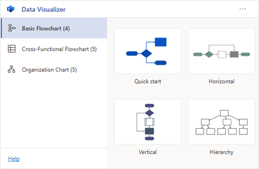
You can create basic flowcharts, cross-functional flowcharts, and organizational charts. The diagrams are drawn automatically from data in an Excel workbook. If you then edit the diagram in Visio, your changes are synced back to Excel.
This means you don’t need a Visio subscription to make stunning diagrams in Excel. View, print, or share your diagrams with others for free in the web version of Visio. For additional editing capabilities, you need either a Visio Plan 1 or Visio Plan 2 subscription.
Note: The Visio Data Visualizer add-in is supported in all the languages supported by Visio for the web. A complete list of the languages is shown at the end of this article.
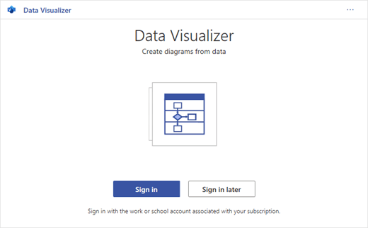
Start with the Visio Data Visualizer add-in
The Data Visualizer add-in is available for Excel on PC, Mac, and the browser with a Microsoft 365 work or school account.
(If the only Microsoft account you have is a personal one—that is, hotmail.com, live.com, outlook.com, or msn.com—you can still try out parts of the Data Visualizer add-in without signing in. It just means that the features available to you are somewhat limited. Read The Data Visualizer add-in is designed for Microsoft 365 work and school accounts for more details.)
-
Open Excel and create a new Blank workbook.
-
Save the workbook to a OneDrive or SharePoint location for seamless sharing and the optimal experience. You can also save your file locally to your computer.
-
Ensure that an empty cell is selected in the workbook.
-
Select Insert > Get Add-ins or Add-ins. In the Office Add-ins Store, search for “Data Visualizer», and then select Add. If you see a security message regarding the add-in, select Trust this add-in.
-
Sign in with the account associated with your Microsoft 365 work or school subscription, or select Sign in later.
In the add-in, we no longer support manual sign-in («ADAL»). But we automatically detect your identity and sign you in. If we can’t sign you in, it means your version of Excel doesn’t work with the add-in. You can fix this by using Excel for the web or upgrading to Excel for Microsoft 365.
Note: When you’re signed in, you unlock capabilities in Visio for the web such as printing, sharing, and viewing in the browser. You don’t need a Visio subscription to use this add-in, but if you have one, you’ll also be able to make edits to your diagram.
If you see a permissions prompt, select Allow.

As an alternative to the procedure above, you can download our add-in ready templates to get started in Excel:
Modify the data-linked table to customize your diagram
-
Choose a diagram type and then select the template you’d like to work with. This will insert a sample diagram and its data-linked table. That process may take a minute. The templates come with different layout and theme options that can be further customized in Visio.
-
If you’re signed in, the diagram is saved as a Visio file in your OneDrive or SharePoint location. If you’re not signed in, then the diagram is part of your Excel workbook instead. You can always choose to create a Visio file by signing in.
-
To create your own diagram, modify the values in the data table. For example, you can change the shape text that will appear, the shape types, and more by changing the values in the data table.
For more information, see the section How the data table interacts with the Data Visualizer diagram below and select the tab for your type of diagram.
-
Add or remove shapes for steps or people by adding or removing rows in the data table.
-
Connect shapes to design the logic of your diagram by entering the IDs of the connected shapes in the corresponding table column for your diagram type.
-
After you’ve finished modifying the data table, select Refresh in the diagram area to update your visualization.
Note: If there is an issue with the source data table, the Data Checker will appear with instructions on how to fix the issue. After you modify the table, select Retry in the Data Checker to confirm the issue is resolved. Then you’ll see the updated diagram.
Tips for modifying the data table
-
Save the Excel workbook (if you’re working in the Visio client) and Refresh frequently.
-
Consider sketching out the logic of your diagram on paper first. This may make it easier to translate into the data table.
View, print, or share your Visio diagram
You can open the Data Visualizer flowchart in Visio for the web to view, print, or share your diagram with others. Learn how:
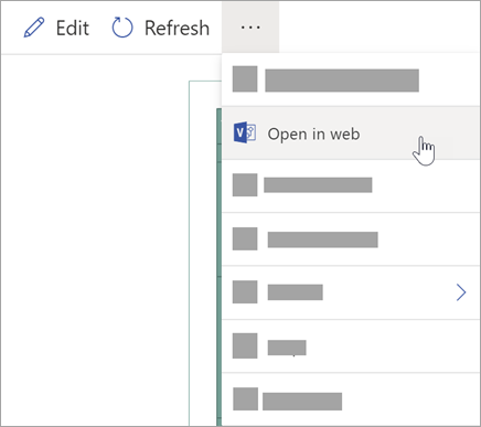
-
To view the diagram outside of Visio for the web, select the ellipses (. . .) in the diagram area and select Open in web.
Note: If you’re not signed in yet, you’ll be prompted to sign in with your Microsoft 365 work or school account.* Select Sign in and then Allow or Accept on any permission prompts.
-
After the Visio file is created, select Open file.
-
In Visio for the web, select the ellipses (. . .) > Print to print your diagram.
-
To share your diagram, select the Share button to create a link or to enter the email addresses of those you want to share with.
Edit the diagram with a Visio subscription
If you have a subscription to Visio, you can do more with the diagram. Add text or images, apply design themes, and make other modifications to customize the diagram.
Do basic editing with Visio for the web
Use Visio for the web for basic editing in the browser, such as changing themes, modifying layouts, formatting shapes, adding text boxes, etc.
-
In the diagram area in Excel, select Edit
.Note: If you’re not signed in yet, you’ll be prompted to sign in with your Microsoft 365 or Microsoft 365 work or school account. Select Sign in and then Allow or Accept on any permission prompts.
-
Make your changes to the diagram in Visio for the web.
To do this
Use
Add and format text
Home > Font options:
For more details, see Add and format text.
Change the theme
Design > Themes
Design > Theme Colors
For more details, see Apply a theme or theme color.
Change the diagram’s layout
Design > Layout
For more details, see Re-layout a diagram.
If you want to add or modify a shape while still keeping the source data in sync, then edit the diagram with the Visio desktop app. Such changes made in Visio for the web can’t by synced back to the Excel source file.
-
When you’re done editing the diagram, go back to the Excel file and select Refresh
to see your changes.
 .
.


 to see your changes.
Do advanced editing with the Visio app
Use the Visio desktop app for advanced edits, such as adding new shapes, modifying connections, and other changes to the structure of the diagram. The Visio app supports two-way sync, so any changes you make can be synced back to your Excel workbook where you can see your diagram changes after refreshing.
Note: To edit in the Visio app, you need a Visio Plan 2 subscription.
-
In the diagram area in Excel, select Edit.
-
Save and close your Excel file.
To edit in the Visio app and successfully sync changes, the Excel file with the data table and diagram must be closed.
-
In Visio for the web select Edit in Desktop App in the ribbon.
-
Select Open to confirm. If you receive a security warning asking if this Visio file is a trusted document, select Yes.
-
Make your changes to the diagram in the Visio app.
-
When you’re done, select the diagram container to see the Data Tools Design tab in the ribbon, and then select Update Source Data.
Note: If you try to update the source data and the link to the Visio data is broken, Visio prompts you to relink. Select the diagram area in Visio, and under the Data Tools Design tab select Relink Source Data. Browse to the Visio workbook with the source table, select Relink, then Update Source Data again.
-
Now that your data has synced back to your Excel workbook, save your Visio file—preferably in the same location as your Excel file.) Close the Visio file.
-
Open the Excel file and select Refresh in the diagram area to see your changes.
Note: If you run into a Refresh Conflict, you can refresh the diagram. You’ll lose any edits you’ve made, but any formatting changes to the shapes or connectors inside the container are preserved.

Microsoft 365 subscribers who have Visio Plan 2 can use Data Visualizer templates to get more advanced diagramming features, such as those listed below. See Create a Data Visualizer diagram for more details:
-
Create a diagram using custom stencils
-
Create sub-processes
-
Bring your diagram to life with data graphics
-
Have two-way synchronization between the data and the diagram
How the data table interacts with the Data Visualizer diagram
Each column of the table uniquely identifies an important aspect of the flowchart that you see. See the reference information below to learn more about each column and how it applies and affects the flowchart.
A number or name that identifies each shape in the diagram. This column is required, and each value in the Excel table must be unique and not be blank. This value does not appear on the flowchart.

This is the shape text that is visible in the diagram. Describe what occurs in this step of the process. Consider also adding a similar or more descriptive text to the Alt text column.

The Process Step ID of the next shape in the sequence. A branching shape has two next steps and is represented by comma-separated numbers such as P600,P400. You can have more than two next steps.
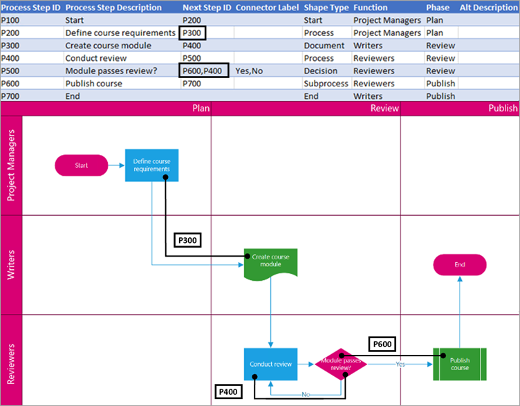
For branching shapes, connector labels are represented as text separated by a comma, such as Yes,No. Yes corresponds to P600 and No corresponds to P400 in the example. Connector labels are not required.
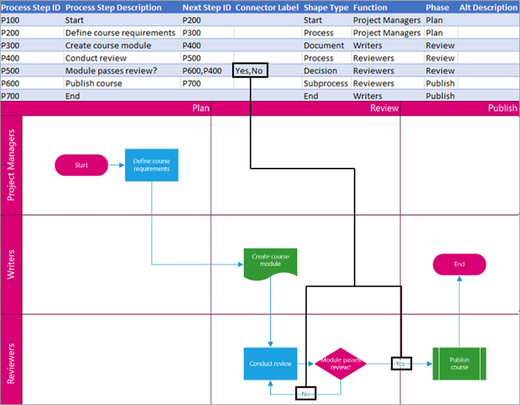
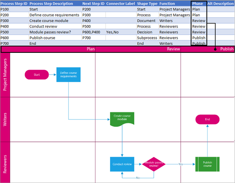
The function (or swimlane) that each shape belongs to. Use the Function and Phase columns to help you organize different stakeholders in your flowchart. This column only applies to a Cross-Functional Flowchart and isn’t included as part of the Basic Flowchart diagram.

The phase (or timeline) that each shape belongs to. Use the Function and Phase columns to help you organize different stakeholders in your flowchart. This column only applies to a Cross-Functional Flowchart and isn’t included as part of the Basic Flowchart diagram.
Alt text is used by screen readers to assist those with visual impairments. You can view alt text you’ve entered as part of the Shape Info of a shape. Entering descriptive alt text is not required, but recommended.
Each column of the table uniquely identifies an important aspect of the organization chart that you see. See the reference information below to learn more about each column and how it applies and affects the diagram.
A number that identifies each employee in your organization chart. This column is required, and each value in the Excel table must be unique and not blank. This value doesn’t appear in the diagram.
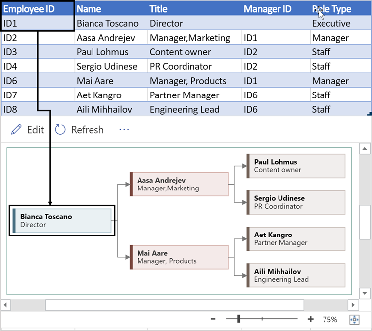
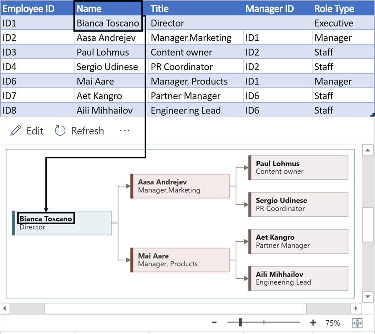
Enter the full name of the employee you want to associate with the employee ID number. This text displays in the diagram as shape text.
Provide additional details for the employee by entering the job title or role. This text displays in the diagram shapes underneath the employee’s name.
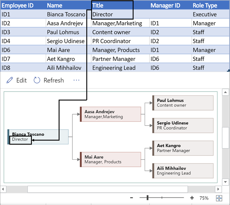
To create the structure of the organization chart, use this column to identify the manager of each employee. You can leave it blank for those who don’t report to anyone. You’ll enter the corresponding employee ID from the first column. You can also separate multiple managers using a comma.
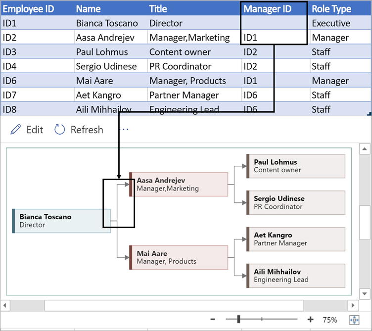
Organization charts in the add-in come with different role types for you to choose from. Select a field under the Role Type column to choose a role that best describes the employee. This will change the color of the shape in the diagram.

Supported languages for the Data Visualizer add-in
Click the subheading to open the list:
-
Chinese (Simplified)
-
Chinese (Traditional)
-
Czech
-
Danish
-
Dutch
-
German
-
Greek
-
English
-
Finnish
-
French
-
Hungarian
-
Italian
-
Japanese
-
Norwegian
-
Polish
-
Portuguese (Brazil)
-
Portuguese (Portugal)
-
Romanian
-
Russian
-
Slovenian
-
Spanish
-
Swedish
-
Turkish
-
Ukrainian
See Also
About the Data Visualizer add-in for Excel
A picture is worth 1,000 words.
Words on pictures are worth millions more.
The aforementioned fact is highly applicable to (us) humans. Multiple scientific researches show that the human brain interprets visual content 60,000 times more than texts and numbers.


Essentially, visual communication is an incredible storytelling tool.
Remember, people remember stories and images more than words and statistics.
Researchers, Data Analysts, and Marketing Managers need to visualize data to communicate meaningful stories to their stakeholders.
Visualization simplifies the communication in the world that involves tons of data. Besides, it communicates the relationships and associations in your data with images.
Given the amount of data generated, you need to be able to interpret increasingly larger batches of data.
“Visualization provides you with insights whenever you find yourself in data wasteland.”
Excel is one of the most-used analytics and data visualization tools by small and medium-sized companies.
However, it lacks a library of custom charts relevant to research, analysis, and marketing management, among other weaknesses, as you shall discover later.
Excel is an incredible tool for data visualization in research and analysis, only when combined with a third-party add-in.
This blog will walk you through time-saving and straightforward steps to visualize your data on Excel, including data visualization examples.
What’s Data Visualization?
Definition: Data visualization is the representation of data or information in a graph, chart, or other visual formats.
In other words, it’s the act of taking information (data) and placing it into a visual context, such as a map or chart.
Visualizing your data makes massive data sets more effortless for the human brain to understand.
A data visualization strategy executed well prioritizes meanings into the massive and complicated paid search marketing campaign datasets.
5 Best Data Visualization Examples Using Excel Spreadsheet
There are over 50 revolutionary and easy-to-read data visualization charts, which are categorized into 6 major sub-groups.
Check them out below. The list is quite long.
Each of the charts has been carefully selected to ensure its 100% relevant.
Coincidentally, ChartExpo is loaded with almost all of them.
I’ll select a single chart example from each sub-group (shown below) and demonstrate how to create highly intuitive and easy-to-read visual storytelling diagrams on Excel using ChartExpo add-in.
Let’s analyze the 5-major chart types on ChartExpo and how you can deploy them quickly.
Let’s dive in without wasting time.
1-Comparative Analysis Charts
Comparative Analysis Charts visualize similarities, differences, and relationships between two or more items based on different parameters.
For example, a simple relationship between ‘keyword A’ and ‘keyword B’ is based on their respective CPC. However, other parameters to consider, such as the clicks per keyword, and impression share, among others.
How would you compare Keyword A and Keyword B based on metrics, such as CPC?
Comparative Analysis Charts are well-positioned to provide you with comparison insights of various dimensions based on particular metrics.
Conduct a ‘health check-up’ on your pay-per-click (PPC) campaigns FREE of charge.
In ChartExpo™, there are various Comparative Analysis Charts that you can use to depict your data story in the best way.
Comparative Analysis Charts on ChartExpo™ include:
- Bar Stacked Comparative Analysis Chart
- Line Comparative Analysis Chart
- Comparison Sentiment Chart
- Comparison Non-Sentiment Chart
- SM Comparison Chart
How do you Generate Comparative Analysis Charts using ChartExpo for Excel?
Remember, the primary aim of drawing charts is to lessen the time and energy that you spend analyzing and drawing inferences from data.
Generation of the charts should also be quick, easy, and less stressful.

Let’s Work with Adjacent Bar Charts for Demonstration Purposes
It is important to check from which device type you are getting the most clicks this will help you to refine your targeting. Adjacent bar chart will help you to analyze this within ChartExpo add-in.
What are the Insights?

With these two metrics set right next to one another, it’s a bit like looking at the two sides of the same coin. It’s a very easy viewpoint to see how each keyword is performing for these two crucial metrics.
Using the sample data, here are some quick insights you can draw:
- Keyword8 is arguably your most valuable target because you have the highest CTR and at a fairly reasonable CPC.
- While Keyword1 looks problematic because of its high CPC, the low CTR means that not many search users are clicking your ads. Thus, you aren’t paying that high CPC too often. This could be a good keyword for generating impressions and brand awareness.
- The real budget eater is Keyword2 because it has a high CTR and a high CPC.
2-Sentiment Analysis Charts
Sentiment Analysis Charts compare products or services to uncover differences. The differences can include categories, such as:
- Quality
- Cost
- Customer satisfaction
The data comparison is represented in the form of columns. Whole columns show all the features of the product or service at a particular time.
The whole columns are then divided into subcategories to show their percentages in the whole. The subcategories can be linked to show their progress over time.
These subcategories are marked with various colors for visual upgrade and easy understanding. Sentiment Analysis Charts can be subdivided into the following:
- Sentiment Trend Chart
- TreeMap Sentiment Chart
- Sentiment Matrix Chart
- Chord Chart
- SM Comparison Chart
- Sentiment Sparkline Chart
Let’s work with some data to simplify your understanding.

How do you Generate Sentiment Analysis Charts using ChartExpo?
Let’s use the Sentiment Matrix Chart for Visualization.
Take a look at the data set as depicted by the screenshot above.
What are the Insights?

From this visualization, you can easily check the feedback about a hospital on different metrics that can help you polish your policies on which you get the negative feedback from your customers. This type of analysis is very helpful to generate good results from your business
3-Specialized Survey Charts
From time to time, seasoned PPC managers conduct surveys to gather the voice of customer (VOC) data for ad targeting purposes.
VOC data is instrumental if you want to personalize ad messages aligned with users’ intent for higher engagement and clicks.
Do you gather VOC data to improve your clients’ PPC campaigns?
If you’re yet to start gathering VOC data, you’re really missing very big.
Don’t worry!
ChartExpo has special survey charts tailor-made for PPC managers to conduct surveys efficiently and in an affordable manner.
Register for ChartExpo Trial NOW to enjoy a 7-days Free Trial
The visualization templates that fall under the broad category of Specialized Survey Charts include:
- Likert Chart
- Score Detail Chart
- Score Bar
- Score Summary Chart
- Rating Bar
- Rating Chart
Let’s visualize our survey data using the Likert Chart to gain insights.
Each bar in the Likert chart represents a survey question. On each survey question, there’s a rating scale (1-5).
The Likert Bar segments have customizable default colors.
How do you Generate Likert Charts using ChartExpo?

Take a look at the sample survey data for a hospital, as depicted by the screenshot above.
Each of the survey questions has a rating scale (1-5).
Each rating has a count, which is the number of people who gave a particular rating. For instance, 324 people provided a 1-star rating on the cleanliness of the hospital.
What are the Insights Generated?

The data set makes sense in the format shown above. The green color denotes a positive response, while red denotes a lower rating.
Overall, the hospital had higher ratings in the key areas respondents were queried during the survey.
The questions: “how do you rate the quality of the hospital staff, and how do you rate your overall experience?” received higher ratings than other questions in the survey.
The most upper bar – the overall bar – represents the summary for all the survey questions.
Each bar has a weighted mean. The chart axis represents the overall percentage.
4-General Analysis Charts
As the name suggests, General Analysis Charts are used for visualizing data in an ordinary manner, such as comparing two metrics over a specific time.
The beauty of these charts is that they are very easy to interpret, irrespective of your analytical skills.
For instance, you can use a world map chart to visualize the contribution of every location targeted by your clients’ ad campaigns.
There are over 30 chart templates in ChartExpo purposely for general analysis.
How cool is this?
The chart templates under General Analysis include:
- Area Chart
- Stacked Area Chart
- Bar Chart Horizontal
- Vertical chart vertical
- Stacked bar chart
- Parallel Bar Chart
Generate Hierarchical Bar Chart with ChartExpo?
This chart presents data in two hierarchy levels. At the top of the chart, there is the share of percentages across all categories. The remaining bars are subcategories.
As a hierarchy, the most relevant data is listed at the top of the chart. By arranging the information in such a way, it is easy to see what’s most significant and takes priority over the other categories
Let’s look at an example.

The data as depicted on the screenshot will be visualized using, Hierarchical Bar Chart which is somewhat familiar to most PPC managers.
What are the Insights?

Using this chart, here are a few insights you can extract:
- Across the board, Google Chrome is the most common browser that people are using.
- Facebook is the #1 social media site for driving traffic.
Understanding how different social media sites and browsers access your content and website can help you better optimize your strategies. You can look at your social media sites with low traffic and determine new ways to boost those channels’ effectiveness.
5-Sankey Charts?
Sankey Diagram provides an overview of the flows in a system, such as a customer journey in search engine marketing (SEM).

This data visualization chart makes it easy to draw actionable insights for optimizing your clients’ Google Ad campaigns.
Sankey charts visually display how clients’ prospects are moving through sales funnels and how their choices and steps coordinate with the ideal way you want the funnels to function.

This chart helps you understand from on which landing page you are getting more users and from which social network. These insights can be used to make the landing pages more attractive and responsive so you can get more users from the social networks.
Why does Visualizing Data Matter?
There’s an interesting relationship between the human brain and visual storytelling.
Essentially, the human brain understands and retains visual story content more easily than mere texts or statistics.
You need data visualization because a visual summary of information makes it easier to identify patterns and trends than looking through thousands of rows on a spreadsheet.
Top 5 Terrific Benefits of Data Visualization
1. Data Visualization Provides Clearer Understanding of the Message
Not only does data visualization help communicate your story to your PPC clients and teams, but it also helps you understand your own story better.
Better, in fact, than any other data analysis tool.
By allowing you to process a large amount of information at once, data visualization opens windows of understanding into the inner workings of your clients’ PPC ad campaigns either by measuring impact or providing actionable visual insight.
Why is this critical to search engine marketing (SEM) management?
As a key decision-maker in your PPC ad agency, you’re not an expert in every activity, but with the proper data visualization comparisons, you can make quicker, more informed decisions.
Just as before, beware of improper comparative visualizations.
If your PPC ad agency’s data analysis objective is unclear, confusing, or complicated, your visualizations might be doing more harm than good.
2. Data Visualization Transform Data into In-depth, Actionable Insights
Spreadsheets are great tools when it comes to collecting and organizing raw data. Visualizations are not a replacement for spreadsheets.
Instead, they are a tool that complements and embellish the data for you to draw meaningful conclusions at just a glance.
Take a close look at the campaign data set below.

Can you make sense of the data?
Exactly, it’s impossible to make meaningful decisions using the data set above.
Let’s visualize the data set.
Note the difference.

Every component is represented and organized in a far better manner. It’s easy to know what’s going on with your clients’ ad campaigns with just a glance.
For instance, Desktop attributes 51.2% of the total ad impressions, which is a critical insight.
Your brain puts the pieces together much faster, thereby giving you more time to put the insights into action!
3. Data Visualization Promotes Insight-Driven Decision Making
Your decision analysis in pay-per-click (PPC) management should be fueled by the data generated by your clients’ PPC ad campaigns.
When you feed accurate, unbiased data visualizations into your decision-making process, you can make better decisions for your PPC business.
If you have a compelling, data-driven story, you’re better equipped to influence the decisions of among your stakeholders (PPC clients and teams)
4. Visualization Reveal Stories Hidden In The Data
Data visualization is an art form often misunderstood by a majority of PPC managers.
It’s not just about creating eye-catching visualizations. It’s about displaying the information in such a way that you convey the insights effectively.
Context is the relevancy that surrounds the data and is necessary to understand the insights.
As a PPC manager, it’s easy to forget about this context because you work with the data often. Clients, however, do not. With the proper visualization, your clients receive all of the information they need to see the whole picture.
Your data has a narrative that you need the visualization to tell.
When you pair the right pay-per-click (PPC) data with the exemplary chart, data storytelling happens.
You’ll be able to convey all of the essential details and underlying trends that would otherwise be lost in the numbers. These patterns, outliers, and other information are vital to getting the insights across to audiences.
5. Data Visualization Reduces Your Costs Instantly
Like I said earlier, PPC ad campaigns generate a massive amount of data, which is less potent without relevant data visualization tools.
PPC managers running multiple accounts would need to hire data scientists to analyze data and compile insights for you.
The salary range of a data analyst in 2020 was between $50,000 and $120,000 per year.
With an intelligent and affordable data visualization solution, you eliminate the need for a data analyst. Coronavirus pandemic is already taking a toll on your agency.
Why would you need extra costs in the current recession?
In light of the above, it makes perfect sense to diagnose your clients’ PPC ad campaigns using intuitive visualization charts.
How To Visualize PPC Ads Campaign Data in Excel?
Excel is one of the most-used tools for analytics by small and medium-sized PPC agencies.
The spreadsheet tool organizes data in columns and rows. Each cell can accommodate different forms of data, such as texts and numbers.
Excel can analyze marketing data and generate basic visual insights using its inbuilt charts.
For example, you could create an Excel spreadsheet that calculates a monthly budget, tracks expenses, or interactively sorts data.
What are the Weaknesses of Excel?
Excel has potentially money-draining weaknesses that could consume your time unproductively and still produce undesirable results.
Firstly, creating specialized charts purposely for PPC management is nearly impossible because Excel lacks intuitive chart templates.
Besides, it’s prone to human error, especially if vast amounts of data are involved.
Secondly, it’s not agile, especially in handling massive amounts of data. Excel is prone to crash, especially if it’s loaded with tons of data.
It’s needless to reinforce that data is gold in today’s digital marketing landscape.
Without data, you cannot access actionable insights to optimize your clients’ pay-per-click (PPC) ad campaigns for desirable results.
Thirdly, visualizing your data using Excel is synonymous with manual PPC management.
Why?
Essentially, it takes a considerable amount of time to visualize your PPC data using Excel without the help of highly efficient and specialized third-party add-ins.
Remember, as a PPC strategist, the last thing you need is a data visualization tool that limits your ability to make maximum use of your massive data.
Creating a custom PPCs chart using Excel is tedious.
Custom PPC charts are data visualization diagrams designed using metrics and dimensions to reinforce accuracy and relevancy.
Lastly, Excel spreadsheet is not collaborative like other tools, such as Excel and a third-party data visualization tool, which I will cover in detail below.
You don’t want to miss the last section.
In light of the Excel revelations above, what’s the solution?
What’s the Solution?
Well, there’s an intelligent and highly affordable Excel add-in that provides in-depth insights in a timely fashion.
This sensational tool accomplishes the mission by diving deeper into your massive search engine marketing (SEM) campaigns data to help you fill in the gaps in your story swiftly.
This Excel add-in is called ChartExpo.
ChartExpo is a fabulous data visualization tool that comes as an add-in for Excel.
Essentially, it turns your Excel into a fantastic data visualization companion capable of simplifying communication and reporting with your stakeholders (clients, colleagues, team etc.).
Mind-blowing Benefits of Using ChartExpo
- ChartExpo has an in-built library with over 50 custom charts designed purposely for pay-per-click (PPC) management.
Guess what?
ChartExpo has all the custom, intuitive charts to:
- Save you money,
- Save you time
- Provide you with a 360-degree view of your clients’ ad campaigns.
- ChartExpo add-in for Excel comes with a free 7-day trial.
Essentially, if you’re not satisfied with the tool within a week, you can opt-out as quickly as signing up for a trial.
- ChartExpo add-in is ONLY $10 a month after the end of the trial period.
It’s cheaper than Starbucks.
- ChartExpo is cloud-hosted, which makes it extremely light. You have a 100% guarantee that your computer or Excel won’t be slowed down.
- When you sign-up for a trial to use ChartExpo, you get a free audit on your clients’ PPC ad campaigns.
The audit results are sent straight away to your email for your reference and action.
- You can export your beautiful, easy-to-read, and intuitive charts in JPEG and PNG, the world’s most-used formats for sharing images.
How to Install ChartExpo add-in on your Excel?
To get started with ChartExpo for Excel add-In, follow the simple and easy steps below.
- Open the worksheet and click the Insert menu button.
- Click the My Apps button and then click the See All, as shown.

- Search for a ChartExpo add-in in the My Apps Store.

- Click the Insert button, as shown above.

- Click the Sign In with Microsoft button link, as shown above.

- Log in with your Microsoft account or create a new account.
- Enter your account and provide ChartExpo with permission to operate in your Excel spreadsheet.
Once you are logged in you will see ChartExpo interface in your sheet.

- Click the Category button on your top right-side to view all the six major categories in ChartExpo.

Wrap Up:
Effective data visualization is the crucial final step of data analytics.
Without it, essential insights and messages will be lost.
With the rise of big data in today’s digital marketing, you really need to be able to interpret increasingly larger batches of data.
There’re multiple revolutionary and amazing custom charts to choose from (as highlighted in the mid-section of the blog post). The main relevant chart categories that come highly recommended for the management includes:
- General Analysis Charts
- Sentiment Analysis Charts
- Comparative Analysis Charts
- Specialized Survey Charts
- PPC Charts
- Sankey
Some of the incredible reasons why you should visualize your data are highlighted below:
- Visualizations reveal stories hidden in the data
- Data visualization provides a clearer understanding of your data.
- It promotes data-driven decision-making.
- Data visualization transform data into in-depth, actionable insights
- Data visualization reduces your costs instantly
The central goal of managers is to help their clients achieve their desired goals and objectives.
This means that paid search managers need a data visualization tool to troubleshoot problems preventing their clients from tapping into the full potential of their search engine marketing (SEM) ads.
Excel is one of the most popular data visualization tools among growing PPC ad agencies due to its responsiveness, ease of use, and, most importantly, its freemium status.
However, it’s time-consuming and mentally exhausting to visualize your campaign data on Excel. Besides, it lacks an in-depth visualization library tailor-made purposely for pay-per-click (PPC) management.
You need a third-party add-in to turn Excel into an intuitive data visualization tool.
In light of the weaknesses of Excel and the vital importance of visualization, you need an affordable tool to get hold of the insights to optimize your clients’ ad campaigns for maximum desired goals at minimal costs.
ChartExpo is easy to install and run on your campaign data irrespective of the magnitude. The intelligent app should be your data visualization partner because of the following money-saving reasons.
- ChartExpo add-in for Excel has an in-built library with over 50 custom charts designed purposely for pay-per-click management.
- ChartExpo add-in for Excel comes with a free 7-day trial. Essentially, if you’re not satisfied with the tool within a week, you can opt out as easily as signing up for a trial.
- ChartExpo is a mere $10 a month after the end of the trial period.
- The money-saving data visualization app is cloud-hosted, which makes it extremely light.
- When you sign-up for a trial to use ChartExpo, you get a free audit on your clients’ PPC ad campaigns.
Sign-up for ChartExpo today to visualize your clients’ campaign data using over 50 custom, revolutionary, affordable, and easy-to-read charts for easy communication with your significant stakeholders-customers and teams.
You have everything to gain and nothing to lose by trying ChartExpo today.