Data validation from excel - Word и Excel - помощь в работе с программами

Note: This is an advanced topic on data validation. For an introduction to data validation, and how to validate a cell or a range, see Add data validation to a cell or a range.

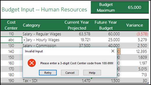
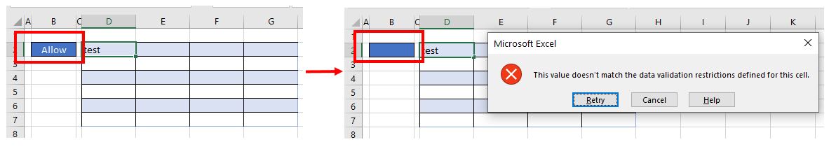
You can use data validation to restrict the type of data or values that users enter into cells. For example, you might use data validation to calculate the maximum allowed value in a cell based on a value elsewhere in the workbook. In the following example, the user has typed abc , which is not an acceptable value in that cell.

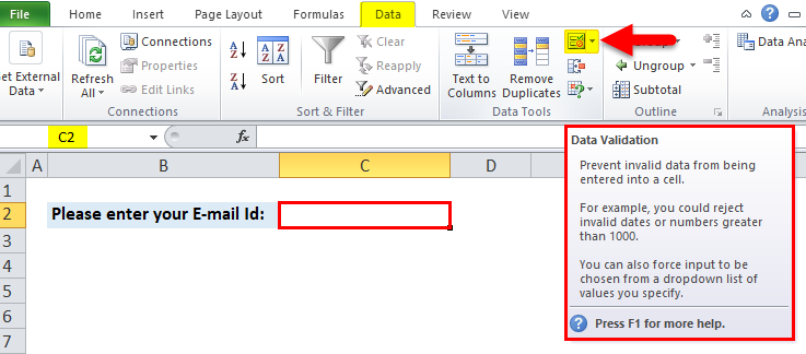
When is data validation useful?

Data validation is invaluable when you want to share a workbook with others, and you want the data entered to be accurate and consistent. Among other things, you can use data validation for the following:

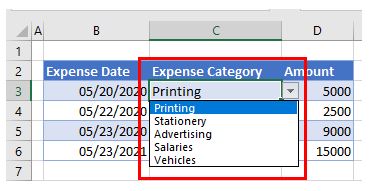
Restrict entries to predefined items in a list— For example, you can limit a user’s department selections to Accounting, Payroll, HR, to name a few.
Restrict numbers outside a specified range— For example, you can specify a maximum percentage input for an employee’s annual merit increase, let’s say 3%, or only allow a whole number between 1 and 100.
Restrict dates outside a certain time frame— For example, in an employee time off request, you can prevent someone from selecting a date before today’s date.
Restrict times outside a certain time frame— For example, you can specify meeting scheduling between 8:00 AM and 5:00 PM.
Limit the number of text characters— For example, you can limit the allowed text in a cell to 10 or fewer characters.
Validate data based on formulas or values in other cells— For example, you can use data validation to set a maximum limit for commissions and bonuses based on the overall projected payroll value. If users enter more than the limit amount, they see an error message.

Data Validation Input and Error Messages

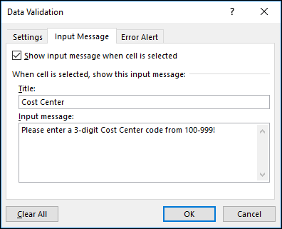
You can choose to show an Input Message when the user selects the cell. Input messages are generally used to offer users guidance about the type of data that you want entered in the cell. This type of message appears near the cell. You can move this message if you want to, and it remains visible until you move to another cell or press Esc.

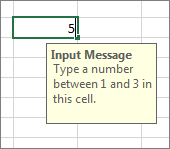
You set up your Input Message in the second data validation tab.

Once your users get used to your Input Message, you can uncheck the Show input message when cell is selected option.

You can also show an Error Alert that appears only after users enter invalid data.

You can choose from three types of error alerts:

Icon	Type	Use to
	Stop	Prevent users from entering invalid data in a cell. A Stop alert message has two options: Retry or Cancel.
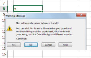
	Warning	Warn users that the data they entered is invalid, without preventing them from entering it. When a Warning alert message appears, users can click Yes to accept the invalid entry, No to edit the invalid entry, or Cancel to remove the invalid entry.
	Information	Inform users that the data they entered is invalid, without preventing them from entering it. This type of error alert is the most flexible. When an Information alert message appears, users can click OK to accept the invalid value or Cancel to reject it.

Tips for working with data validation

Use these tips and tricks for working with data validation in Excel.

Note: If you want to use data validation with workbooks in Excel Services or the Excel Web App you will need to create the data validation in the Excel desktop version first.

The width of the drop-down list is determined by the width of the cell that has the data validation. You might need to adjust the width of that cell to prevent truncating the width of valid entries that are wider than the width of the drop-down list.
If you plan to protect the worksheet or workbook, protect it after you have finished specifying any validation settings. Make sure that you unlock any validated cells before you protect the worksheet. Otherwise, users will not be able to type any data in the cells. See Protect a worksheet.
If you plan to share the workbook, share it only after you have finished specifying data validation and protection settings. After you share a workbook, you won’t be able to change the validation settings unless you stop sharing.
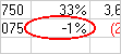
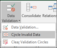
You can apply data validation to cells that already have data entered in them. However, Excel does not automatically notify you that the existing cells contain invalid data. In this scenario, you can highlight invalid data by instructing Excel to circle it on the worksheet. Once you have identified the invalid data, you can hide the circles again. If you correct an invalid entry, the circle disappears automatically.

To apply the circles, select the cells you want to evaluate and go to Data > Data Tools > Data Validation > Circle Invalid Data.
To quickly remove data validation for a cell, select it, and then go to Data > Data Tools > Data Validation > Settings > Clear All.
To find the cells on the worksheet that have data validation, on the Home tab, in the Editing group, click Find & Select, and then click Data Validation. After you have found the cells that have data validation, you can change, copy, or remove validation settings.
When creating a drop-down list, you can use the Define Name command (Formulas tab, Defined Names group) to define a name for the range that contains the list. After you create the list on another worksheet, you can hide the worksheet that contains the list and then protect the workbook so that users won’t have access to the list.
If you change the validation settings for a cell, you can automatically apply your changes to all other cells that have the same settings. To do so, on the Settings tab, select the Apply these changes to all other cells with the same settings check box.
If data validation isn’t working, make sure that:
- Users are not copying or filling data — Data validation is designed to show messages and prevent invalid entries only when users type data directly in a cell. When data is copied or filled, the messages do not appear. To prevent users from copying and filling data by dragging and dropping cells, go to File > Options > Advanced > Editing options > clear the Enable fill handle and cell drag-and-drop check box, and then protect the worksheet.
- Manual recalculation is turned off — If manual recalculation is turned on, uncalculated cells can prevent data from being validated correctly. To turn off manual recalculation, go to the Formulas tab > Calculation group > Calculation Options > click Automatic.
- Formulas are error free — Make sure that formulas in validated cells do not cause errors, such as #REF! or #DIV/0!. Excel ignores the data validation until you correct the error.
- Cells referenced in formulas are correct — If a referenced cell changes so that a formula in a validated cell calculates an invalid result, the validation message for the cell won’t appear.
- An Excel table might be linked to a SharePoint site — You cannot add data validation to an Excel table that is linked to a SharePoint site. To add data validation, you must unlink the Excel table or convert the Excel table to a range.
- You might currently be entering data — The Data Validation command is not available while you are entering data in a cell. To finish entering data, press Enter or ESC to quit.
- The worksheet might be protected or shared — You cannot change data validation settings if your workbook is shared or protected. You’ll need to unshare or unprotect your workbook first.

How to update or remove data validation in an inherited workbook

If you inherit a workbook with data validation, you can modify or remove it unless the worksheet is protected. If it’s protected with a password that you do not know you should try to contact the previous owner to help you unprotect the worksheet, as Excel has no way to recover unknown or lost passwords. You can also copy the data to another worksheet, and then remove the data validation.

If you see a data validation alert when you try to enter or change data in a cell, and you’re not clear about what you can enter, contact the owner of the workbook.

Need more help?

You can always ask an expert in the Excel Tech Community or get support in the Answers community.

Источник

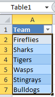
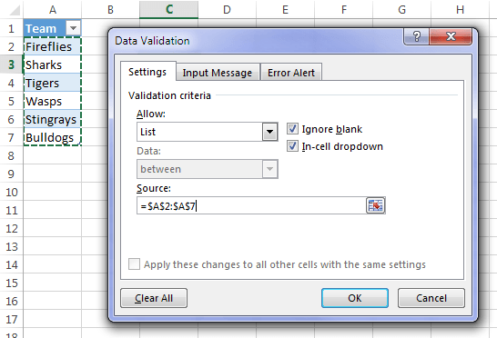
I’ve set up a table with some team names that I want to use in a Data Validation list.

The reason I formatted my list in an Excel table is because I want the range to dynamically update when I add or remove teams from the list.

My table’s name is Table1, as you can see here in the name box:

Now, if you’ve ever tried to reference an Excel Table as your Data Validation lists source like this:

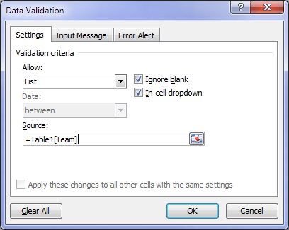
Then you probably got the error:

“The formula you typed contains and error”.

Here are three ways to fix this:

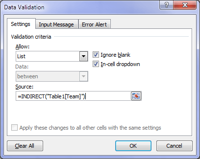
Method 1: Use the INDIRECT function with the tables structured references like this:

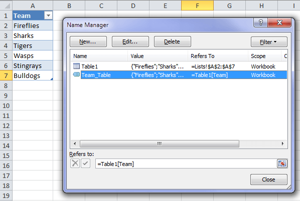
Method 2: Give your Table another name in the name manager. In this example my table is in cells A2:A7 and is called Table1. In the name manager I’ve set up a new named range called Team_Table and referenced it to the Team column (and only column in this case) of Table1:

Now I can set up my Data Validation list like this:

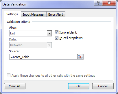
No need to use INDIRECT, and it will still dynamically update as new data is added or removed from the table just like the first example.

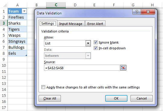
Method 3: Simply reference the cells in the table:

Then when you add items to the bottom of the Table your Data Validation List source automatically updates*, almost like magic. No named range, no Structured references:

It’s a shame you can’t just use the Table Structured Reference as your Data Validation list source. I suspect this is a bug/oversight. Unfortunately I’m not aware of any plans to fix it and it’s still like this in Excel 2016!

*Note: this requires the Table to be on the same sheet as the data validation list. If not, use method 2.

Источник

The data validation in excel helps control the kind of input entered by a user in the worksheet. In other words, the input typed in a specific cell must comply with the criteria set for that cell. Data validation also allows providing instructions to the user about the input to be typed. The cell to which the data validation rule is applied is called a validated cell.

For example, the following data validation rules can be created in certain cells of Excel:

A whole number between 1 (minimum) and 20 (maximum) is allowed.
A date is allowed to be entered which is greater than September 15, 2000 (start date) or lesser than September 15, 2020 (end date).
A text entry is allowed which matches any of the values (“yes,” “no,” and “cannot say”) of a drop-down list.

The pointers “a,” “b,” and “c” are the validating criteria defined for certain cells. If the input in these cells does not correspond to the respective pointer (a, b, or c), an error alert message is displayed by Excel.

Apart from setting the criteria, data validation in excel also allows to create a pre-defined range of inputs (drop-down list). In such cases, the user is asked to select the appropriate option (input) from this range. This ensures that all the data entries follow the same format.

Since the entries of all users are standardized, data validation brings about consistency and reduces errors. The “data validation” option is available in the “data tools” group of the Data tab of Excel.

What is Data Validation in Excel?
- How to Use Data Validation in Excel?
  - Example #1–“Data Validation” Window Explained
  - Example #2–Decimal Number Validation
- Data Formats in Data validation
- The Different Validation Criteria
- The Different Error Alert Styles
- Purpose of Data Validation in Excel
- The Limitations of Data Validation in Excel
- Frequently Asked Questions
- Recommended Articles

How to Use Data Validation in Excel?

Let us consider some examples to understand the working of the data validation feature of Excel.

You can download this Data Validation Excel Template here – Data Validation Excel Template

Example #1–“Data Validation” Window Explained

The following image shows a list of numbers in column B. We want to perform the following tasks:

Show how to create a data validation rule on the range B1:B4.
Explain the tabs of the “data validation” window.

The steps explaining the creation of a data validation rule in Excel are listed as follows:

Select the cells on which the data validation rule has to be created. So, select the range B1:B4.
Click the data validation drop-down (in the “data tools” group) from the Data tab of Excel. The same is shown in the following image.
Select “data validation” from the drop-down list.
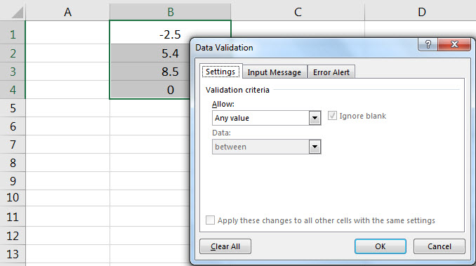
The “data validation” window appears, as shown in the following image.
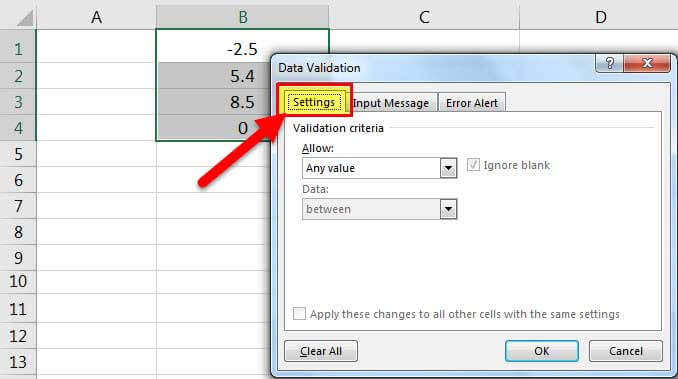
The first tab is “settings,” which contains the validation criteria. The same is shown in the succeeding image.
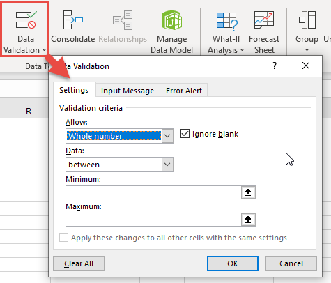
From the drop-down list under “allow,” one can select the data format allowed to the users. The drop-down list under “data” is used for defining the criteria.

For instance, if the input should be entered as a whole number, select the same from the drop-down list under “allow.” Once “whole number” is selected, one can choose the minimum and the maximum range between which this number is allowed to be entered.

Likewise, the desired validation criteria can be defined for the user.

Note: Refer to the topics “The Different Data Formats” and “The Different Validation Criteria” of this article for more information on adding validation criteria.
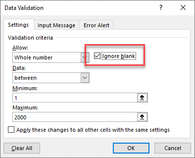
The checkbox “ignore blank” is selected by default. This selection tells Excel to ignore the blank values.
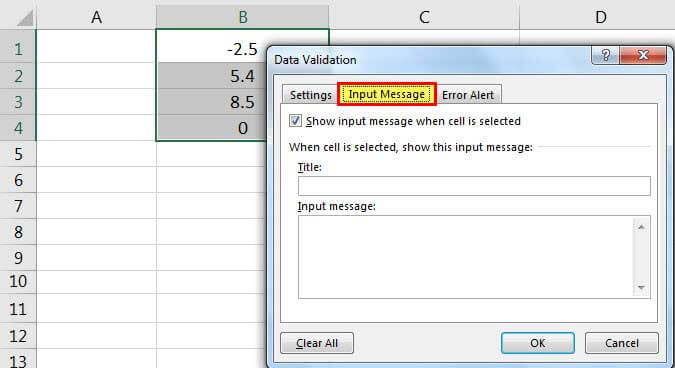
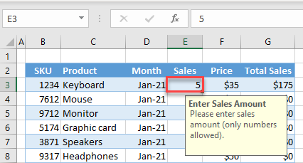
The second tab is “input message,” as shown in the succeeding image. One can enter the “title” and the “input message,” which are displayed when a validated cell is selected.
Note: An “input message” tells the user about the kind of input allowed in a validated cell. However, it is optional to add an input message. But, if one does add an input message, ensure that the checkbox of “show input message when cell is selected” is checked.
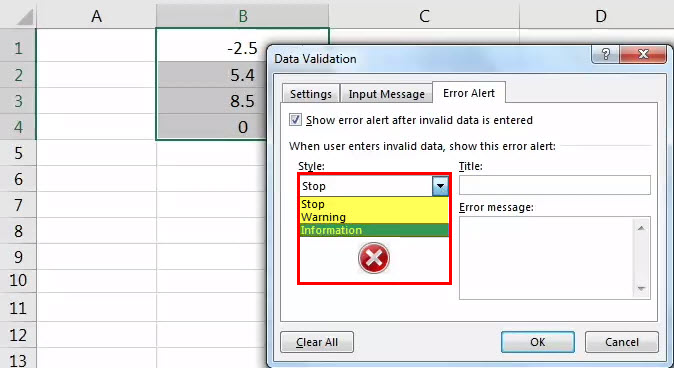
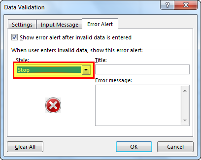
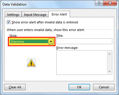
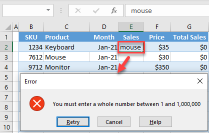
The third tab is “error alert.” In this tab, one can enter the “title” and the “error message” that are displayed on typing invalid data in the validated cell.
From the “style” drop-down, one can select any of the three options, “stop,” “warning” or “information.” These are shown in the succeeding image.

Note 1: An “error message” is a customized message which tells the user that he/she has made an error while typing data in the validated cell. However, it is optional to add an error message. If an error message is added, ensure that the checkbox of “show error alert after invalid data is entered” is checked.

Note 2: In case an error message is not added, Excel displays the default error message, which states that restrictions have been defined for the validated cell.

Note 3: For more information on the error alert styles, refer to the topic “The Different Error Alert Styles” of this article.
Once the entries in the three tabs, “settings,” “input message,” and “error alert” have been defined, click “Ok” in the “data validation” window.
The data validation excel rule is applied to the selected range B1:B4. Likewise, one can create a data validation rule by selecting either a single cell or a range of cells in Excel.

Note: For creating a data validation rule, it is mandatory to enter the validation criteria in the “settings” tab (step 5). However, it is optional to define the tabs “input message” (step 7) and “error alert” (step 8).

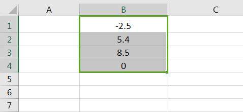
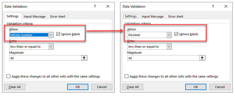
Example #2–Decimal Number Validation

Working on the data of example #1, we want to perform the following tasks:

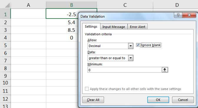
Create a data validation excel rule on cell B1. In this cell, a decimal number greater than or equal to zero is allowed to be entered.
Define an input message which appears on selecting cell B1. The title should be “negative number detected” and the message should be “enter number greater than zero.”

The steps for performing the stated tasks are listed as follows:

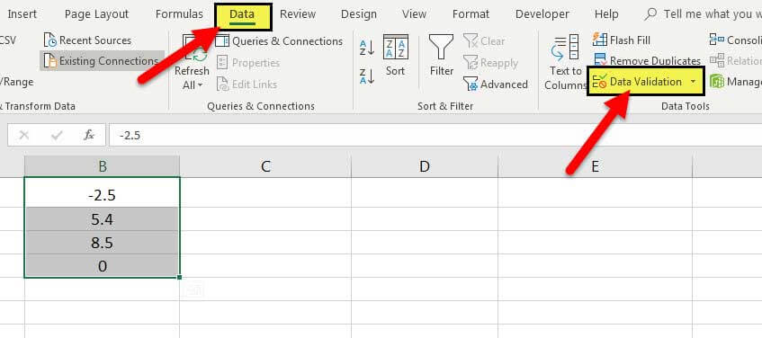
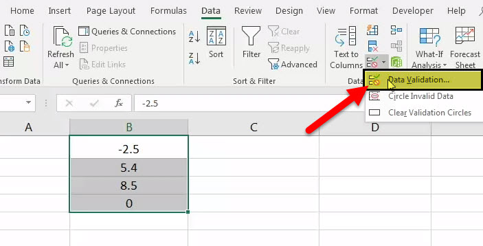
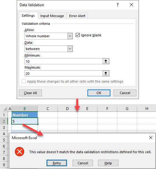
Step 1: Select cell B1 which contains -2.5. From the Data tab of Excel, click the “data validation” drop-down. Select “data validation.”

Step 2: The “data validation” window appears, as shown in the following image. In the “settings” tab, select “decimal” under the “allow” drop-down.

Under the “data” drop-down, select “greater than or equal to.” In the box under “minimum,” enter “0” (without the double quotation marks).

Step 3: In the “input message” tab, select the checkbox of “show input message when cell is selected.”

In the box under “title,” type “negative number detected” without the double quotation marks. In the box “input message,” type “enter number greater than zero.” This should also be written without the double quotation marks. Click “Ok.”

The data validation rule is created on cell B1. To cross-check it, select the validated cell B1. The defined input message appears, as shown in the following image.

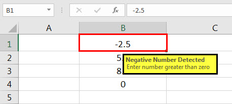
The number -2.5 was already there in cell B1 before the creation of the validation rule. This number is not deleted (from cell B1) even after creating a data validation rule.

However, in future, if a number is entered in cell B1, it must conform to the newly created rule. This implies that a decimal number greater than or equal to zero can be entered in cell B1. So, negative numbers are restricted in this cell. In case this rule is not complied with, Excel will display the default error alert.

Data Formats in Data validation

While entering data in a validated cell, there are certain formats that are allowed to the user. The rule creator (who is creating the data validation rule) can pick any of these formats based on which a validation rule can be created.

In the “settings” tab of the “data validation” window, the “allow” drop-down shows the following formats:

Any value: This implies that no validation will be executed. In case a data validation rule is created and then “any value” is selected, the created validation rule is removed. However, the input message of the created validation rule can be viewed even after “any value” has been selected.
Whole number: This requires that the user should enter a whole number in the validated cell.
Decimal: This implies that the data format allowed in the validated cell is decimal numbers.
List: This implies that the format allowed is a drop-down list. So, a drop-down list consisting of pre-defined values needs to be created. This drop-down list can be created in any of the following ways:
- Supply the values directly in the box under “source.”
- Provide the reference to the range (in the “source” box), which consists of the required values.
- Enter the name of the named range (in the “source” box), which begins with an “equal to” (=) sign.

Date: This implies that the user can enter only a date in the validated cell.
Time: This implies that a time value should be entered in the validated cell.
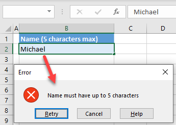
Text Length: This helps fix the number of digits or text entered in a validated cell. For instance, the user can enter either numbers or text up to 5 digits or 5 characters respectively.
Custom: This allows one to create a formula. This formula is used to validate (restrict) the input entered by the user. For instance, a formula can be entered to ensure that a text entry ends with certain characters, the text should be in uppercase or the entry must only be numeric, etc.

The Different Validation Criteria

Excel presents different criteria for validating data. The rule creator can select any of these criteria. Based on this selection, one can set the limits within which the input is allowed.

In the “settings” tab of the “data validation” dialog box, the drop-down under “data” shows the following validating criteria:

Between: This implies that the input should be between the minimum and the maximum numbers specified.
Not between: This implies that the input should not be between the minimum and the maximum numbers specified.
Equal to: This implies that the input should be equal to the specified value. In other words, the input should be the same as the specified value.
Not equal to: This implies that the input should not be equal to the specified value. In other words, the input should be different from the specified value.
Greater than: This implies that the input should be greater than the minimum number specified.
Less than: This implies that the input should be lesser than the maximum number specified.
Greater than or equal to: This implies that the input should be greater than or equal to the minimum number specified.
Less than or equal to: This implies that the input should be lesser than or equal to the maximum number specified.

The Different Error Alert Styles

There are different error alert styles in Excel. The rule creator can select any of these styles to notify the user that an error has been made while typing data in the validated cell.

In the “error alert” tab of the “data validation” window, the drop-down under “style” presents the following options:

Stop: This stops the users from entering invalid data in the validated cell. With the “stop” style, the error alert message presents the following main options to the user:
- Retry– Clicking “retry” allows typing a new input.
- Cancel–Clicking “cancel” deletes the invalid input.

The “stop” style is the default error alert style of Excel.

Warning: This warns the users that an invalid input has been entered. However, it does not stop the user from entering incorrect data. With the “warning” style, the user is presented with the following main options:
- Yes–Clicking “yes” makes Excel accept the invalid input.
- No–Clicking “no” allows typing a new input.
- Cancel–Clicking “cancel” deletes the invalid input.

Warning

Information: This informs the user that the input entered is invalid. Like the “warning” style, this also does not stop the user from entering incorrect data. With the “information” style, the user is presented with the following main options:
- Ok–Clicking “Ok” makes Excel accept the invalid input.
- Cancel–Clicking “cancel” deletes the invalid input.

By selecting a style, its respective icon appears in the error alert message displayed by Excel.

For instance, with the “stop” style, the cross within the red circle is shown (in the error alert message) as the user enters invalid data. Likewise, with the “warning” and “information” styles, the exclamation mark (within a yellow triangle) and the “i” sign (within a blue circle) show up respectively.

Note: Apart from the main options listed (in the preceding pointers 1, 2, and 3), Excel also displays the “help” option in all the error alert messages, irrespective of the style selected.

Purpose of Data Validation in Excel

The objectives of data validation in excel are listed as follows:

To restrict the users from entering unwanted or incorrect data values in the worksheet
To sort and study the data obtained with the help of defined criteria
To suggest the valid data format to the users through customized input messages (displayed when a validated cell is selected)

Excel Data validation is particularly helpful in the following situations:

When the number of users is large and there is a possibility of entering inputs in different formats
When the allowed entries need to be defined with a drop-down list
When an error alert (warning message) needs to be displayed on entering invalid data

The Limitations of Data Validation in Excel

The limitations of data validation in excel are listed as follows:

Data validation in excel does not prevent a user from copying an incorrect input from a non-validated cell to a validated cell. It can stop one from typing an incorrect input but not from copying the same. Hence, the purpose of data validation can become pointless if a user copies and pastes an invalid input.
Excel Data validation cannot fully protect a worksheet from invalid data entries. If a user copies an incorrect input from a non-validated cell and pastes it in a validated cell, the validation rule in the latter cell is eliminated. As a result, the validation rule is absent on the copied data.

Frequently Asked Questions

1. Define data validation in Excel.

Data validation restricts (limits) the type of input entered by a user in the worksheet. One can set the criteria for a specific cell and ensure that the input typed (in that cell) complies with it.

For instance, in cell A1, one is allowed to type only a decimal number between 1.5 and 9.5. This is a data validation rule applied to cell A1 of the worksheet.

2. How can a data validation rule be edited in Excel?

Let us say that rule X has been applied to cells A1 and D1. We want to change this to rule Y for both the mentioned cells.

The steps to edit a data validation rule are listed as follows:

a. Select any of the cells to which rule X has been applied.
b. Select “data validation” from the “data validation” drop-down (in the “data tools” group) of the Data tab.
c. In the “settings” tab of the “data validation” window, enter the new criteria as per rule Y.
d. Select the checkbox of “apply these changes to all other cells with the same settings.” This ensures that rule Y is applied to both the cells A1 and D1.
e. Click “Ok.”

The rule Y has been applied to both cells A1 and D1.

Note: The new data validation rule can be applied to all the validated cells only if they all had the same validation criteria initially. In this case, the initial validation criterion (rule X) was the same for both the validated cells (A1 and D1).

3. How can a data validation rule be removed in Excel?

The steps to remove (delete) a data validation rule are listed as follows:

a. Select the validated cell.
b. From the “data validation” drop-down (in the “data tools” group) of the Data tab, select “data validation.”
c. The “data validation” window opens. In the “settings” tab, click “clear all” appearing at the bottom left side.
d. Click “Ok.”

The validation rule will be cleared from the selected cell (selected in step a).

Note: To remove the same validation rule applied to multiple cells, select the checkbox of “apply these changes to all other cells with the same settings.” Thereafter, click “clear all” followed by “Ok.”

Data Validation in Excel

Data validation is a feature in MS Excel used to control what a user can enter in a cell of an excel sheet. Like, restrict entries in a sheet, such as a date range or whole numbers only. We can even create dropdowns as well, which saves un-necessary space and shows the values in a single cell. Also, we can create a customized message which will appear user insert any incorrect value or an incorrect format.

As an example, A user can specify a meeting scheduled between 9:00 AM and 6:00 PM.

As we can use data validation in excel to make sure a value is a positive number, a date between 15 and 30, make sure a date occurs in the next 30 days, or make sure a text entry is less than 25 characters etc.

Locate in MS Excel

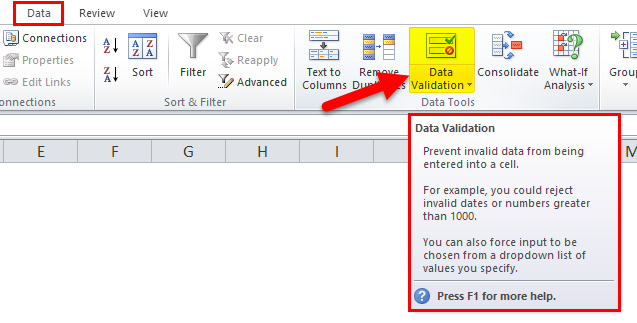
Click on Data Tab in the Menu bar.

Select on Data Validation from the toolbar under the Data Tab:

How to Create Data Validation Rule in Excel?

Let us understand the working of Data validation in excel by some examples.

You can download this Data Validation Excel Template here – Data Validation Excel Template

Example #1

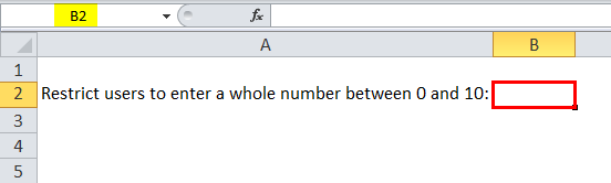
We can restrict a user to enter a whole number between 0 and 10.

Execute the Below mention steps for the creation of the data validation rule in excel:

Step 1: Select B2 Cell.

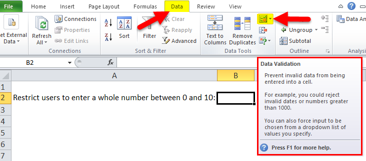
Step 2: Go to the Data tab, click on Data Validation from Data in the toolbar.

Step 3: A data validation Pop-Up will open:

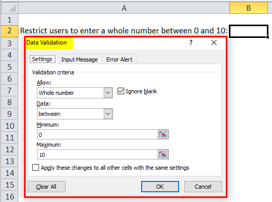
Step 3.1: On the Settings tab, Click on Allow drop-down under validation Criteria.

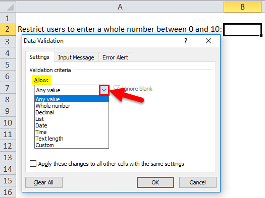
Step 3.2: Select the Whole number, then Some more required options will be enabled.

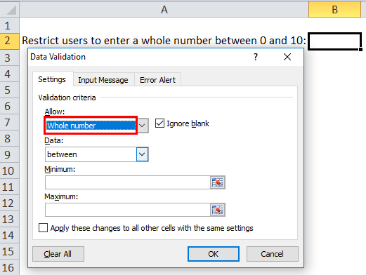
Step 3.3: Select between from the drop-down of the Data list, Enter the Minimum and Maximum number for restriction. And click ok.

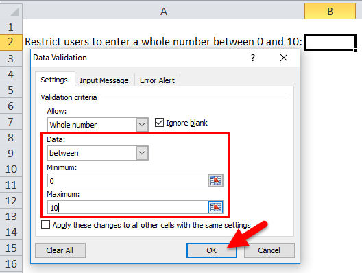
Step 3.4: All settings will apply to the selected cell.

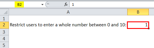
Now Enter 1 in cell B2- It will allow a user to enter any whole number from 0 to 10.

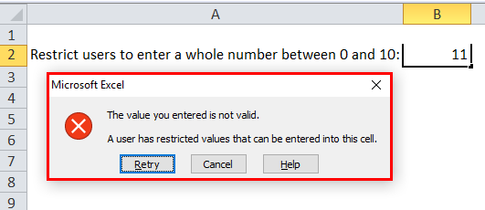
Now Enter 11 in cell B2- It will throw by default error.

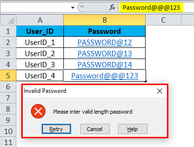
Example #2 – Set Input Message and Error Alert

We can restrict a user to enter a limited text.

Step 1: Select B5 Cell from Example 2 Sheet.

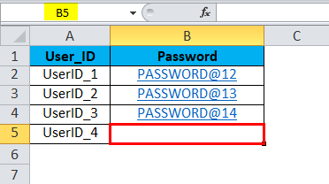
Step 2: Click on the data validation tool from the Data Menu Bar and select Text Length in Allow drop-down.

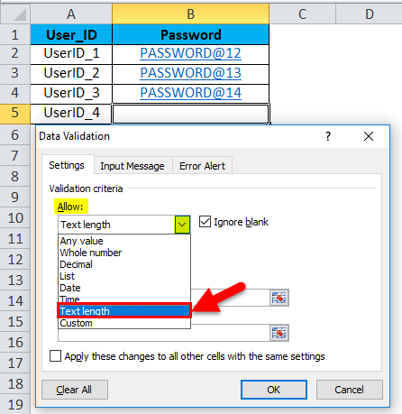
Step 3: Select equal to from the data list drop-down.

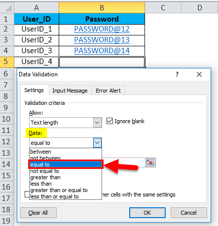
Step 4: Enter your desired length of the password (as an example 11).

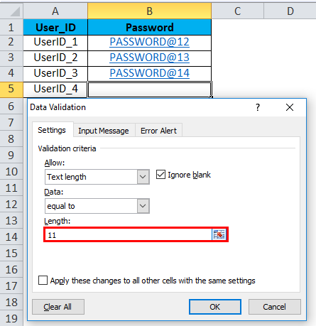
Step 5: Click on the Input Message tab and provide a message displayed on the selection of cell.

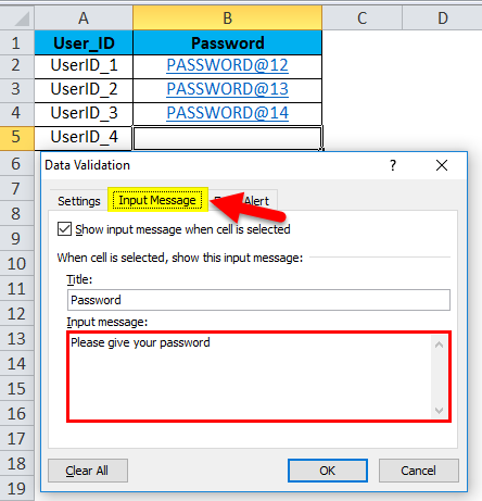
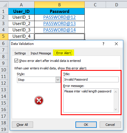
Step 6: Click on the Error Alert tab, provide a Title and the Error message, which will be displayed if a user entered an invalid length password.

Step 7: After that, click the Ok button, the setting will be applied to the selected cell.

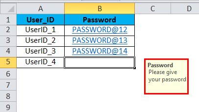
On the Selection of Cell, an Input message will be displayed.

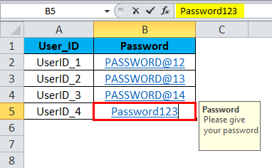
Enter a text which has a text length of 11. It will be selected successfully.

Now enter an invalid password. It will throw the described error message.

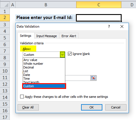
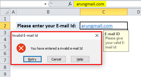
Example #3 – Custom option for e-mail address validation

Step 1: Select the C2 cell, Go to Data Tab and click on Validation data in the toolbar.

Step 2: Select custom in Allow drop-down.

Step 3: Write a formula for selecting only value if it is having ‘@’.

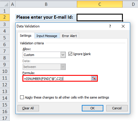
Step 4: Click on the Input Message tab, provide the message, which will be displayed on the selection of a cell.

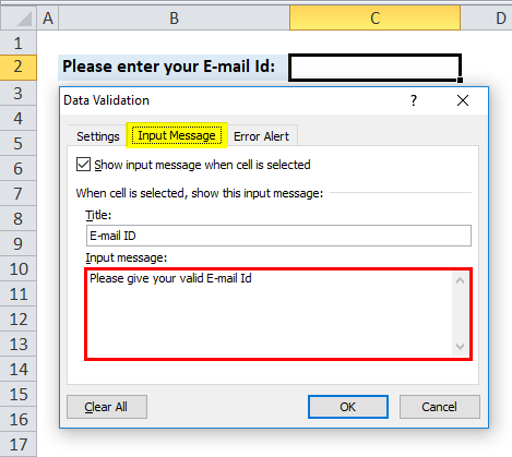
Step 5: Click on the Error Alert tab, provide the Title and an Error message, which will be displayed if a user entered an invalid length E-mail Id.

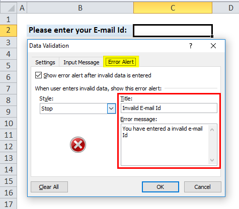
Step 6: After that, click the Ok button, the setting will be applied to the selected cell.

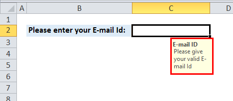
On the Selection of Cell, the Input message will display.

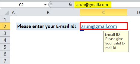
Enter a valid e-mail id – It will be selected successfully.

Now enter any invalid e-mail Id- It will throw a described error Message.

Valuation criteria of excel data validation Settings

Any Value – To provide any type of data.
Whole Number – Enter only whole numbers.
Decimal – Enter only decimal numbers.
List – Pick data from the drop-down list.
Date – Accept the only date.
Time – Enter only time.
Text Length – Fixed the length of the text.
Custom – Enter a custom formula.

Conditions in data list in Valuation criteria settings

Between, not between, equal to, not equal to, greater than, less than, greater than or equal to, less than or equal to.

Some more condition of excel data validation Settings

If a user wants to ignore the blank, then there is a checkbox called Ignore.
If a user selects between, then a user needs to select the Minimum and Maximum values for the cell(s).
If a user wants to apply these changes to all other cells with the same setting, then there is a checkbox that needs to mark, and it will apply to the remaining cells in the sheet.

When to Use Data Validation in Excel?

Best used when a user wants to share a sheet with another user, and he wants the data entered to be accurate and consistent.
Restrict entries to predefined items in a list.
Restrict numbers outside a specified range.
Restrict dates outside a certain time frame.
Restrict times outside a certain time frame.
Limit the number of text characters.
Validation of the data, which is available on other sheets or workbook.
Choose to be displayed an Input Message when a user clicks on a cell as a user’s guide.
A user can customize the error alert; it can be anything as per a user-defined.

Things to Remember About Data Validation in Excel

If a user wants to create a data validation rule in the workbook for excel web apps or Excel services, then he needs to create an excel data validation rule on the desktop first.
If one user sender a workbook to another, then first, a user needs to make sure that the workbook is unlocking; otherwise second, a user is never able to access the workbook cells to fill value.
Always make in mind that there is no error in a formula like #REF! or #DIV/0!
Anyone who can create a data validation rule in the filled cell MS excel will not detect it.

How to Remove the Excel Data Validation rule?

A user can remove excel data validation from a cell, select the cell, click Data Validation, and then click Clear All.

A user can modify or delete the excel data validation rule only if the inherited sheet is unprotected. If it is password protected, contact the owner of the workbook. Only he can help to unprotect the workbook. As there is no way to recover or lost the password option in MS Excel.

Use Drop-Down Lists

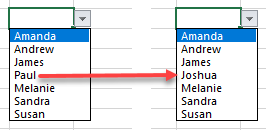
The most useful type of data validation is the drop-down list feature. For instructions on creating a drop-down list, see Create or Add a Drop-Down List in Excel and Google Sheets.

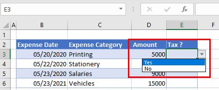
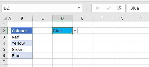
There are plenty of uses for drop-down lists and many ways to create them. For example, a simple yes/no drop-down list like the one below can be added as a quick and dependable indicator in a spreadsheet.

You can also use VBA to create a drop-down list in a cell. Enter this code in the VBA editor:

Sub DropDownListinVBA()
Range("A2").Validation.Add Type:=xlValidateList, AlertStyle:=xlValidAlertStop, _
Formula1:="Orange,Apple,Mango,Pear,Peach"
End Sub

Dynamic Drop-Down Lists

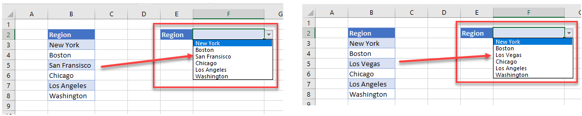
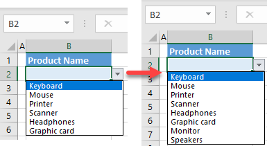
When you create a drop-down list based on a range of cells using a data validation rule, if the data in that specific range changes, then the values in the drop-down list also change.

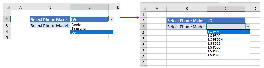
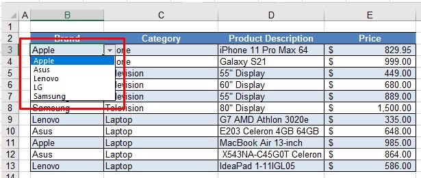
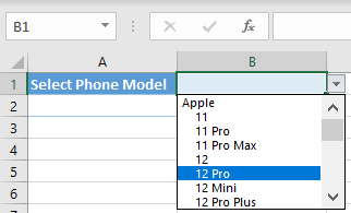
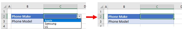
Go a step further with a cascading drop-down list based on the value that is selected in a different list. In the example below, the user has selected LG as the Phone Make. The list of Phone Models then shows only the LG models. If the user were to select either Apple or Samsung, then the list would change to show the relevant models for those makes of phone.

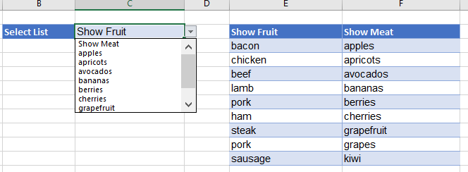
An alternative method is to use an IF statement within the data validation feature to show a specific list that changes according to what the user selects. In the example below, if the user selects Show Fruit, then the fruit drop-down list is shown, whereas selecting Show Meat brings up the meat drop-down list.

Filter Data With a Drop-Down List

You can use Excel’s filter tool alongside a drop-down list for extended functionality.

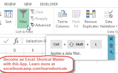
Filters and drop-down lists are similar and even use the same keyboard shortcut (CTRL + SHIFT + L). In a data validation context, the shortcut activates a drop-down menu.

A drop-down list can also be used as a filter in Excel. It enables you to extract rows of data that match the entry in the drop-down list and return these rows to a separate area of the worksheet.

Drop-Down List Formatting and Display Tools

If you want to create a drop-down list where the background color depends on the text selected, you can use Conditional Formatting to amend the background color when an item from the list is selected.

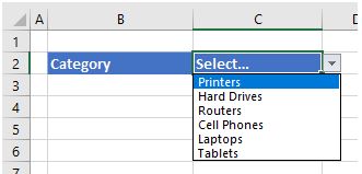
When you create a drop-down list, the default value of the cell where you have placed the list is usually blank. It can be useful to pre-populate this cell with either a default value or a message to the user, such as Select…

Once you’ve created a drop-down list, you can use the SORT and UNIQUE Functions to sort the drop-down list into alphabetical order.

To make a drop-down list more readable, you can group a list of items by category (phone models in brand groups, for example).

AutoComplete Drop Down

AutoComplete is a useful feature of Excel in that it can reduce the number of characters you need to type in each cell. The standard data validation drop-down functionality does not support AutoComplete. However, you can learn here how to approximate autocomplete with a drop-down list. Then, when you start typing the first letters of an entry in the drop-down list, the rest of the entry automatically shows up.

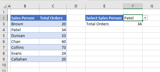
Drop Down Populates Another Cell

Selecting an item from a drop down can populate a different cell in Excel and Google Sheets. For example, in the graphic below, Patel is selected from the list, and the cell below is then populated with the value 34. You can learn how to do this by clicking here.

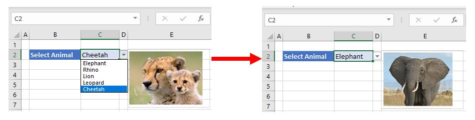
Using a drop-down list, you can also insert a picture into another cell automatically.

Data Validation Based on Another Cell

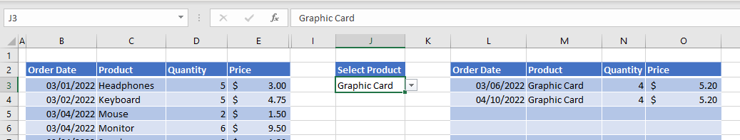
When entering values in Excel, you can restrict the data that is entered into any range of cells based on text or a value held in another cell.

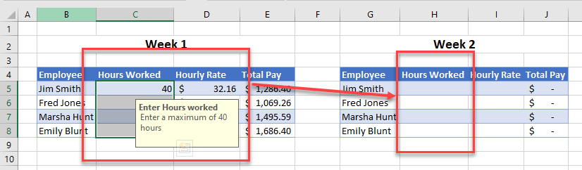
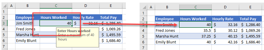
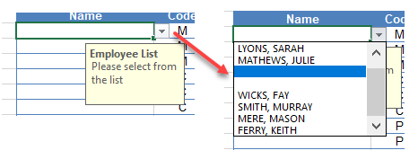
When you create a drop-down list, you can write a custom input message that is seen on the screen when a cell is selected. This input message can also be referred to as a ToolTip.

You can also customize the output (error alert) message that is returned to the user if invalid data is entered into a cell.

Options and Settings

There are seven different data types you can select from the Allow box of the Validation criteria: Whole number, Decimal, List, Date, Time, Text length, and Custom.

The Ignore blank option is only available if you are actually editing a cell that has that option switched off.

You can also choose, when editing a data validation rule, whether or not to apply the changes to other cells with the same settings.

Date and Time Formats

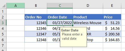
You can use Data Validation to restrict the format entered into a cell to ensure it is a date, and also to restrict the entry to be set between a start date and an end date.

Set a Character Limit

In Excel, the number of characters allowed in a single cell is 32767. However, you can set your own character limit for a text cell.

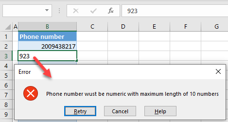
Validate Phone Numbers and Emails

You can use Data Validation to ensure that a phone number is entered correctly into Excel.

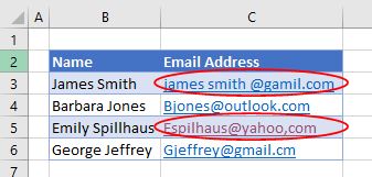
You can also use Data Validation to ensure that an email address contains a @ sign and does not have any spaces or commas in it.

Custom Formulas

You can write a custom formula to make your own data validation rules. In the example below, the formula ensures that the data in a cell begins with certain text.

Custom Formula Examples

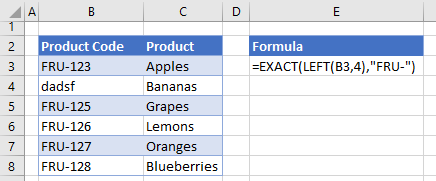
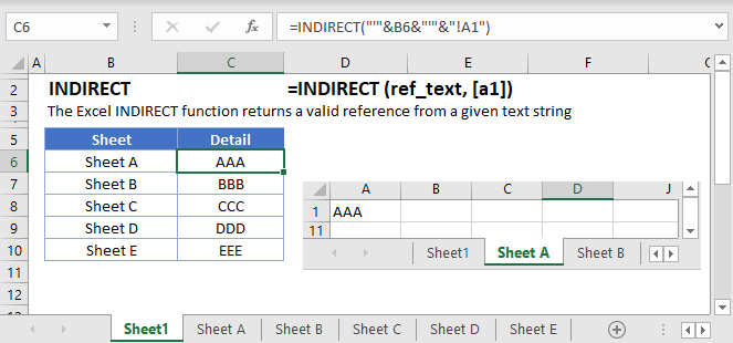
You can use the INDIRECT Function in Excel in conjunction with a data validation drop-down list to create a cell reference from text.

Use the ISNUMBER Function to check that the data inputted is in fact, a number. Data Validation has a built-in Whole number option, but you can generalize further with a custom formula.

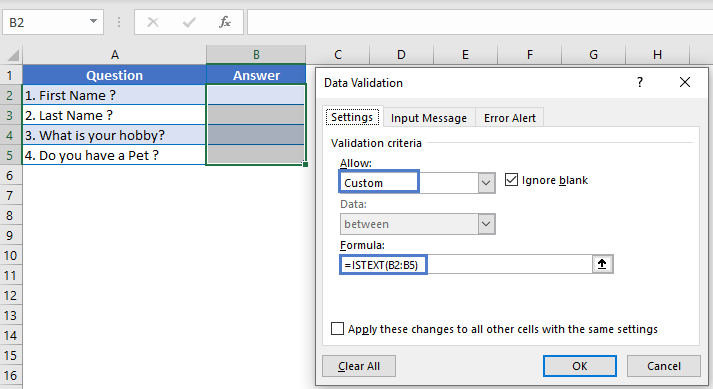
Use a the ISTEXT Function to check for text. The example below allows only text values in the cells with data validation applied.

You can use a data validation drop down with the COUNTIF Function to count cells that meet certain criteria and return a total.

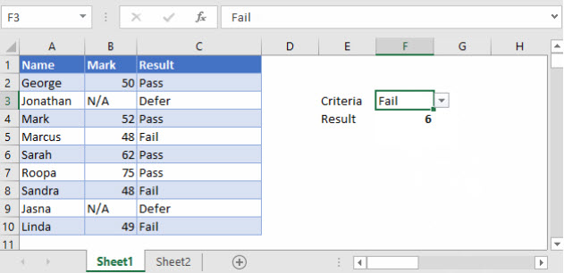
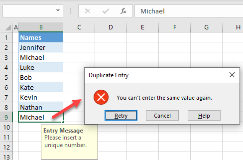
COUNTIF is also useful for preventing users from entering duplicate values.

A risk score matrix is a matrix that is used during risk assessment in order to calculate a risk value by inputting the likelihood and consequence of an event. You can use a data validation drop down in conjunction with the VLOOKUP and MATCH Functions to create a risk score matrix.

Change or Remove Data Validation Rules

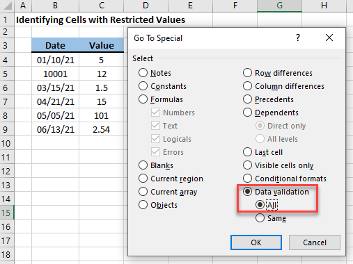
If you have a data validation rule set in Excel, you can find any restricted values by selecting Data validation in the Go To Special dialog box.

You can copy data validation rules from one set of cells to another set of cells by using the Paste Special command (CTRL + ALT + V).

If you already have rules set up in a worksheet, you can amend the validation rules should your requirements change.

You can amend the contents of a drop-down list by following the instructions in this tutorial.

You can easily update (change, extend, or have fewer items) a drop-down list by adding or deleting items from the list’s source range.

If data validation on a range is no longer required, you can remove it.

If you no longer require a drop-down list, you can easily remove the data validation settings by following the instructions in this tutorial.

Issues and Fixes

If you have a value in Google Sheets that does not match the items in your drop-down list (an invalid item), you get a red triangle in the top left corner of the cell. To get rid of this triangle, you can follow the steps in this tutorial.

There are a number of reasons why your data validation rule or drop-down list is not working correctly. You can troubleshoot these issues by referring to this tutorial.

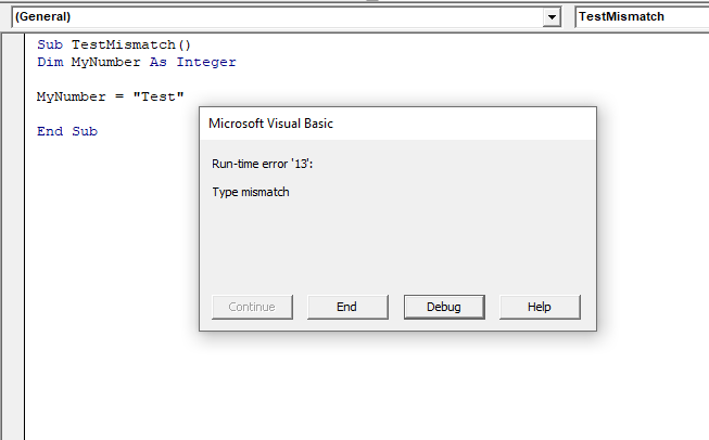
A mismatch error can occur when you run VBA code. The error stops your code from running completely and flags the error by means of a message box. One of the ways you can prevent this from happening is to use Data Validation on the spreadsheet to prevent the user from causing worksheet errors in the first place. Only allow them to enter values that don’t cause worksheet errors.

Источник

When is data validation useful?

Data Validation Input and Error Messages

Tips for working with data validation

How to update or remove data validation in an inherited workbook

Need more help?

Table of contents

How to Use Data Validation in Excel?

Example #1–“Data Validation” Window Explained

Example #2–Decimal Number Validation

Data Formats in Data validation

The Different Validation Criteria

The Different Error Alert Styles

Purpose of Data Validation in Excel

The Limitations of Data Validation in Excel

Frequently Asked Questions

Recommended Articles

Data Validation in Excel

How to Create Data Validation Rule in Excel?

Example #1

Example #2 – Set Input Message and Error Alert

Example #3 – Custom option for e-mail address validation

Valuation criteria of excel data validation Settings

Conditions in data list in Valuation criteria settings

When to Use Data Validation in Excel?

Things to Remember About Data Validation in Excel

How to Remove the Excel Data Validation rule?

Recommended Articles

Use Drop-Down Lists

Dynamic Drop-Down Lists

Filter Data With a Drop-Down List

Drop-Down List Formatting and Display Tools

AutoComplete Drop Down

Drop Down Populates Another Cell

Data Validation Based on Another Cell

Options and Settings

Date and Time Formats

Set a Character Limit

Validate Phone Numbers and Emails

Custom Formulas

Custom Formula Examples

Change or Remove Data Validation Rules

Issues and Fixes