Data validation excel duplicates

This example teaches you how to use data validation to prevent users from entering duplicate values.

1. Select the range A2:A20.

2. On the Data tab, in the Data Tools group, click Data Validation.

3. In the Allow list, click Custom.

4. In the Formula box, enter the formula shown below and click OK.

Explanation: The COUNTIF function takes two arguments. =COUNTIF($A$2:$A$20,A2) counts the number of values in the range A2:A20 that are equal to the value in cell A2. This value may only occur once (=1) since we don’t want duplicate entries. Because we selected the range A2:A20 before we clicked on Data Validation, Excel automatically copies the formula to the other cells. Notice how we created an absolute reference ($A$2:$A$20) to fix this reference.

5. To check this, select cell A3 and click Data Validation.

As you can see, this function counts the number of values in the range A2:A20 that are equal to the value in cell A3. Again, this value may only occur once (=1) since we don’t want duplicate entries.

6. Enter a duplicate invoice number.

Result. Excel shows an error alert. You’ve already entered that invoice number.

Note: to enter an input message and error alert message, go to the Input Message and Error Alert tab.

See all How-To Articles

This tutorial demonstrates how to prevent duplicate entries in Excel and Google Sheets.

Prevent Duplicate Entries

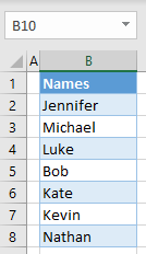
If you want to allow only unique values in a column, use the data validation functionality in Excel. This way, you can prevent a user from entering duplicate values. Say you have the following list of names in Column B.

To prevent duplicate entries in a range, follow these steps:

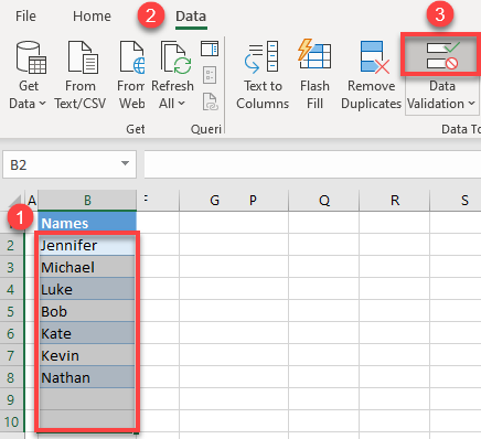
1. Select the range for data validation (e.g., B2:B10), and in the Ribbon, go to Data > Data Validation.

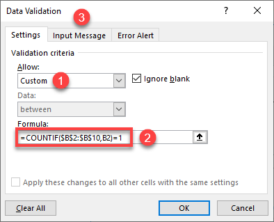
1. In the Data Validation window, (1) select Custom as the validation criteria under Allow, and (2) enter the COUNTIF formula:

=COUNTIF($B$2:$B$10,B2)=1

This formula counts – for each entry – how many times that value appears in the range B2:B10. If the result is 1 (meaning the entry appears only once in the range) then it is allowed. Otherwise, the data validation rule prevents a user from entering that value, since it is already in the range.
Then (3) go to the Input Message tab.

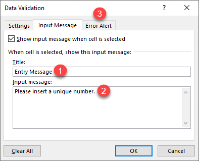
1. In the Input Message tab, enter (1) the Title of the message you’re adding and (2) the Input message. This message appears when a user selects a cell in the data validation range to provide information about the data validation rule.
   Then (3) go to the Error Alert tab.

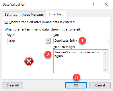
1. In the Error Alert tab, enter (1) the Title of the error message and (2) the Error message. This message appears if a user enters an existing value and prevent them from entering duplicate values.
   Then (3) click OK.

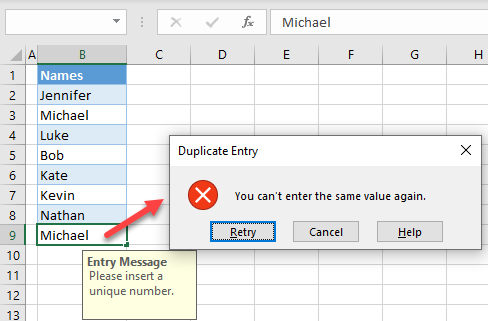
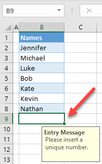
Now selecting an empty cell from the data validation range (for example, B9) prompts an input message about data validation.

If you try to enter an existing value in cell B9 (e.g., Michael), you get the error message pictured below, stopping you from entering a duplicate value.

Note: To remove duplicate values or duplicate rows that were already present in the data, see How to Remove Duplicate Cells or this VBA tutorial.

Prevent Duplicate Entries in Google Sheets

To prevent duplicate entries in Google Sheets, follow these steps.

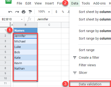
1. Select the range for data validation (e.g., B2:B10), and in the Menu, go to Data > Data validation.

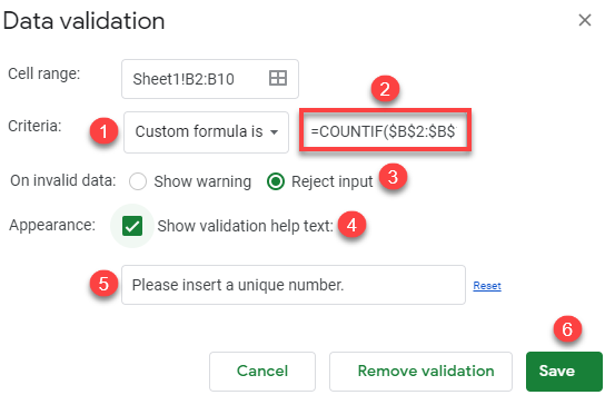
1. In the Data validation window, (1) enter Custom formula is as the Criteria, and (2) enter the formula:

=COUNTIF($B$2:$B$10,B2)=1

Then (3) select Reject input, (4) check Show validation help text, and (5) enter an error message. (6) Click Save.

Now, if you try to enter a value in cell B9 that already exists in the range, you get the error message you just set.

Author: Oscar Cronquist Article last updated on April 21, 2020

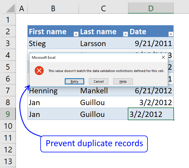
This article demonstrates how to set up Data Validation in order to control what the Excel user is allowed to enter. The condition is that there can’t be two identical records in the Excel Table.

The image above shows a warning that the Excel user tried to enter a duplicate record which is not valid, the dialog box tells you that «This value doesn’t match the data validation restrictions defined for this cell.

There are three buttons available, «Retry», «Cancel» and «Help» on the dialog box. The «Retry» button leaves the value as it is but selected, this allows you to edit the value you just entered. The «Cancel» button removes the value you just entered. The «Help» button opens a web page at Microsoft Support explaining how Data Validation works.

Create an Excel Table

An Excel Table allows you to dynamically apply Data Validation to new data meaning if you enter a new record below the data set it will also have the same data validation rules automatically as the rest of the data.

With this setup there is no need to adjust cell ranges when new data is added or deleted, the Excel Tables does that for you instantly.

1. Select any cell in the data set.
2. Press shortcut keys CTRL + T to open the «Create Table» dialog box, see image above.
3. Enable/disable checkbox «My table has headers» accordingly.
4. Press with left mouse button on «OK» button to apply settings and create an Excel Table.

The data set is now an Excel Table which you can tell by the cell formatting and the arrows next to column headers. You can change the Excel Table style and remove «Filter» arrows next to column headers if you want.

A new tab on the ribbon named «Table Design» appears if you select on any cell in the Excel Table, it allows you to change Table Options and Styles.

Apply Data Validation

Data Validation lets you control what the Excel user can and can’t enter using different methods. We are going to use a «Data Validation» formula that will trigger a dialog box warning if conditions are not met.

1. Select data in your Excel Table, I selected cell range B3:D9.
2. Go to tab «Data» on the ribbon.
3. Press with left mouse button on «Data validation» button.
   
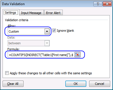
4. Choose Custom, see image above.
5. Type in «Formula:» field:

   =COUNTIFS(INDIRECT(«Table1[First name]»), $B3, INDIRECT(«Table1[Last name]»), $C3, INDIRECT(«Table1[Date]»), $D3)<=1

6. Press with left mouse button on OK button to apply settings and create «Data Validation» to cell range B3:D8

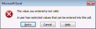
If you enter a duplicate record, the following error message appears.

Explaining the data validation formula in row 9

To learn how formulas work in greater detail I recommend the «Evaluate Formula» tool which is built-in to Excel, you can use this tool for «Data Validation» formulas as well. Copy the «Data Validation» formula and paste to a cell.

I pasted the formula to cell F3 and then pressed Enter. Select cell F3, press with left mouse button on tab «Formulas» on the ribbon. Press with left mouse button on «Evaluate Formulas» button to show the «Evaluate Formula» dialog box, see image above.

The INDIRECT function is a volatile function meaning it recalculates every time Excel recalculates, this may make it more cpu-intensive if used extensively. This function is needed in order to reference values to an Excel Table in a Data Validation formula.

This is why you get the warning text «A function in this formula causes the result to change each time the spreadsheet is calculated. The final evaluation step will match the result in the cell, but interim steps may not» in the «Evaluate Formula» dialog box, see image above.

Underlined expressions are what is about to be evaluated in the next step and italic values are the result. Press with left mouse button on the «Evaluate» button to move to the next calculation step in the formula. Press with left mouse button on «Close» button to dismiss the dialog box.

Step 1 — How to reference values in Excel data validation formulas

You can’t reference Excel Tables in Data Validation formulas, however, there is a workaround. The INDIRECT function allows you to reference Excel Tables.

References to Excel Tables are called «structured references» and they don’t change when values or records are added or deleted in the Excel Table.

Table1[First name]

becomes

INDIRECT(«Table1[First name]»)

The downside is that you need to change the formulas if you change the Table name or the Table header names accordingly, they do not change automatically in this case.

Step 2 — Count how many times a record exists in a table

The COUNTIFS function lets you count cells based on multiple conditions, we are going to count rows based on the values the Excel user enters in the Excel Table.

COUNTIFS(criteria_range1, criteria1, [criteria_range2, criteria2]…)

We will use as many criteria pairs (ranges and criteria) as there are columns in the Excel Table. I will use six arguments as there are three columns in my Excel Table. You need to adjust that to your specific Excel Table.

COUNTIFS(INDIRECT(«Table1[First name]»), $B3, INDIRECT(«Table1[Last name]»), $C3, INDIRECT(«Table1[Date]»), $D3)

becomes

COUNTIFS($B$3:$B$9, $B3, $C$3:$C$9, $C3, $C$3:$D$9, $D3)

becomes

COUNTIFS({«Stieg»; «Jonas»; «Camilla»; «Lars»; «Henning»; «Jan»}, $B3, {«Larsson»; «Jonasson»; «Läckberg»; «Kepler»; «Mankell»; «Guillou»}, $C3, {40807; 41324; 41215; 40777; 41081; 40970}, $D3)

becomes

COUNTIFS({«Stieg»; «Jonas»; «Camilla»; «Lars»; «Henning»; «Jan» ; «Stieg»}, «Stieg», {«Larsson»; «Jonasson»; «Läckberg»; «Kepler»; «Mankell»; «Guillou»; «Larsson»}, «Larsson», {40807; 41324; 41215; 40777; 41081; 40970; 40807}, 40807)

and returns 1 in cell F3.

Step 3 — Check if number is smaller than or equal to 1

The less than sign and the equal sign together means that the number must be equal to or less than 1 in order to return True.

COUNTIFS(INDIRECT(«Table1[First name]»), $B3, INDIRECT(«Table1[Last name]»), $C3, INDIRECT(«Table1[Date]»), $D3)<=1

becomes

1<=1

and returns TRU. The «Data validation» error message does not appear.

Recommended articles

• Block duplicate entries in Excel table
• Apply data validation to cells

• Software

Today I finally decided to make an Excel dashboard on debtors aging analysis. The main reasons to do this dashboard were that:

1. I thought now enough knowledge has been delivered to my cult followers that they will understand the ins and outs of making this dashboard; and
2. that majority of computational work was already done in the shape of my old tutorial where learnt how to make aging analysis report in Excel.

But soon it was dawned upon me that not everything has already been discussed that is needed. So consider this article to be the second article of the Aging Analysis Dashboard Series. The first one being the base article in which aging calculation was done.

As with any dashboard the list of requirements was developed and one of such requirement was to get the data validated list of customers. It was seemingly easy task as I have already discussed how to create drop-down lists using data validation lists in many of my articles.

So here is what I did:

But things were NOT so simple and a big question mark dropped on my head when I clicked the drop down arrow button. Have a look at the result and see what kind of list I got. That is definitely not what we wanted:

So why it happened. If you download the file and open it you will see that customers’ names are repeated as in reality we can have many transactions with the same customer in a period. Also the data is sorted according to the date transaction occurred and not according to customers’ names. So we have two problems now:

1. One: the data is unsorted and that will make lists ugly as lists are meant to be in alphabetical order.
2. Two: We have duplication of names because of multiple transactions with the same customer. So if we use this data the same customer will be listed multiple times in the list whereas one customer should be listed only once.

Though we can easily fix the first problem by sorting the data. But the second problem is still there.

Use Remove Duplicate Tool

One way is to copy the whole column containing customers’ names in another column or worksheet and run Remove duplicates command from the ribbon. Following animation shows how this command works:

This will leave us with unique values and we can use them to make our drop down list. Which we can use to make drop down list as the following animation shows:

But this approach has one serious caveat. Well at least I consider it really serious and that is what if data grows in the future and more customers are added? In that case we will have to create new drop down list every time a transaction takes place with a new customer.

So this is a plausible solution but not a good one. I needed a more dynamic and future proof approach and I found that solution is pivoted on Excel’s Pivot Tables.

Pivot Tables + Data Validation = Awesome Lists!

I must say that Pivot tables are not really used for this purpose but so far data validation tools is still without an option to consider only unique values and ignore duplicates like we have an option to ignore blanks.

So the basic idea is that we will make a small pivot table containing just customers’ names. Pivot tables are awesome in so many ways but one no TWO great deals about it are:

1. It removes the duplicates automatically and only fetch unique values as it can count the repetitive entries and take them as one.
2. It sort the data in alphabetical order automatically.

So this ONE solution is automatically solving TWO of our problems. But we still need to learn:

• firstly how to make the required pivot table? and
• secondly how to get the drop-down list on the basis of this pivot table?

Follow these steps to get this done:

Step 1: Select the data containing customers, dates, invoice numbers and amounts by hitting Ctrl+A and convert it to a Table by hitting Ctrl+T. A dialogue box will show up. Make sure “my table has headers” option is ticked. Click OK. This will make our source dynamic and anything based on this table will also be dynamic.

Step 2: Select the table again if it is not selected and go to Insert tab > Tables group > click Pivot table button. This will invoke create pivot table dialogue box. You can give it a name and choose it to be on existing worksheet or new. Just ignore and simply click OK button. This will move you to new worksheet with pivot table options.

Step 3: From the options above left click HOLD and drag the value to rows box below. This will get you customers’ names sorted and without repetition.

Step 4: Have an active cell inside pivot table, go to Design tab > layout group > click grand totals drop-down > click off for rows and columns. This will remove the grand total row from pivot table.

Step 5: Right click on the worksheet tab and rename it to pivot.

Step 6: Now go to the cell where you want drop down list. I want it to be on the same worksheet where my original data is. Go to Data tab > Data tools group > click data validation tool button. This will open up data validation dialogue. From allow drop down select list and in source input field put this formula:

=OFFSET(pivot!$A$4,0,0,COUNTA(pivot!$A:$A)-1)

Following animation also shows how this formula is actually put in place.

Now as I said that data input source is dynamic so if add any new customer and refresh the pivot table my drop down list will update automatically and thus saves me the hassle of doing the whole process again.

But remember once the underlying data is changed you have to refresh the pivot table.

So here you are one step closer to make your first ever Excel dashboard. We will be continuing on Aging analysis dashboard from this point in the future.

Don’t forget to checkout more of our articles on:

• Excel pivot tables
• Uses of data validation tool