Data table in what if analysis in excel

There are some Microsoft Excel features that are awesome but somewhat hidden. And the «data table analysis» is one of them.

Sometimes a formula depends on multiple inputs, and you’d like to see how different inputs values would impact the result. The data table is perfect for that situation.

This is extremely useful to analyze a problem in Excel and figure out the best solution.

The Dataset

To use the data table feature we will need some data.

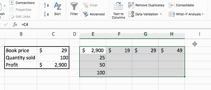
Here’s a table with 2 inputs (book price and quantity sold), and a formula (revenue = price * quantity).

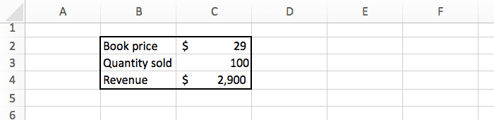
If we sell 100 books at $29 each, we will make $2,900.

The data above assume we know the book price and how many copies we will sell. But we’re actually not sure, so we’d like to know the revenue for different combination of price and quantity. For example: how much profit will we make if we sell 150 copies instead of 100, and what if the price is $19 or $49?

There are 2 main ways to do that:

Manually change the 2 inputs, and see how the result change.
Do that automatically with the data table feature.

Nobody likes doing repetitive tasks manually, so let’s try the second option

The Set Up

Before we start using the data table, we need to do some changes to our data.

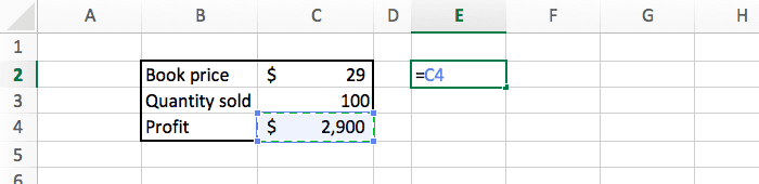
First we need to copy the formula to a separate place. You can do this by simply typing =C4 in a blank cell.

Then we need to tell Excel what values we would like to test. To the right of the formula we list all the prices ($19, $29, $49), and below the formula we list all the quantities (25, 50, 100).

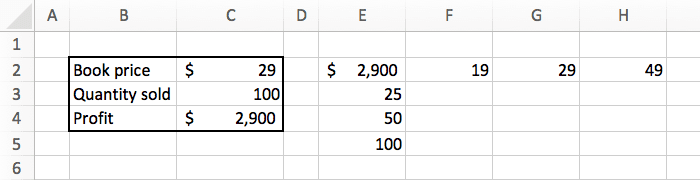
And we can add some basic formatting (borders and currency) to make things look slightly better.

Our goal is to fill this table with the profit for each combination of price and quantity.

Data Table Example

Now we can start the interesting part!

Select the new table we just created, and in the «data» tab, click on the «what if analysis» button. There select «data table».

A popup will appear that you need to fill like this:

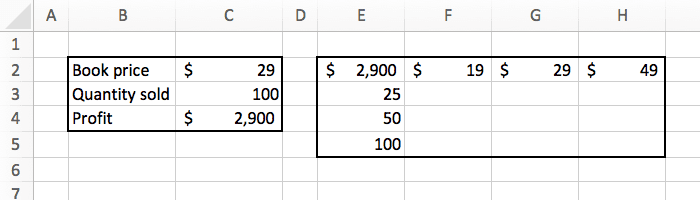
Row input cell: we listed the price at the top, so the «row input» is the price, which is in C2.
Column input cell»: we listed the quantity in the left, so the «column input» is the quantity, which is in C3.

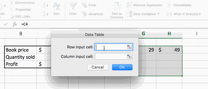
Press OK, and we are done. Excel did the math for us, and automatically updated the spreadsheet with all the numbers we wanted.

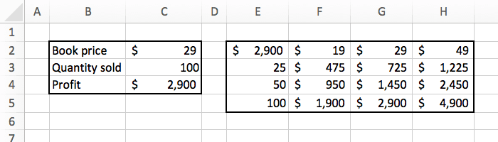
Now we can see exactly how much revenue we will make based on the different combination of inputs. For example it shows that selling 50 copies at $49 will make us $2,450. That’s super powerful.

Limitations

For your information, using data tables have some drawbacks. Here I listed three limitations that make me most uncomfortable:

The performance and calculation speed of an Excel file will be slowed down if it contains many data tables.
The structure of the data table is fixed. You will get an error message if you try to insert a row or column in a data table, or if you delete just a single cell in it.
The data table must be located on the same tab as the setup data table (as mentionned above in the Set Up section). You cannot link the data table to cells on a different tab.

Conclusion

With just a few clicks, we can get Excel to do some magic computation and give us interesting information.

For this example we had a simple formula. But you could do the same on something much more complex, and Excel will give you the perfect answer in no time.

Источник

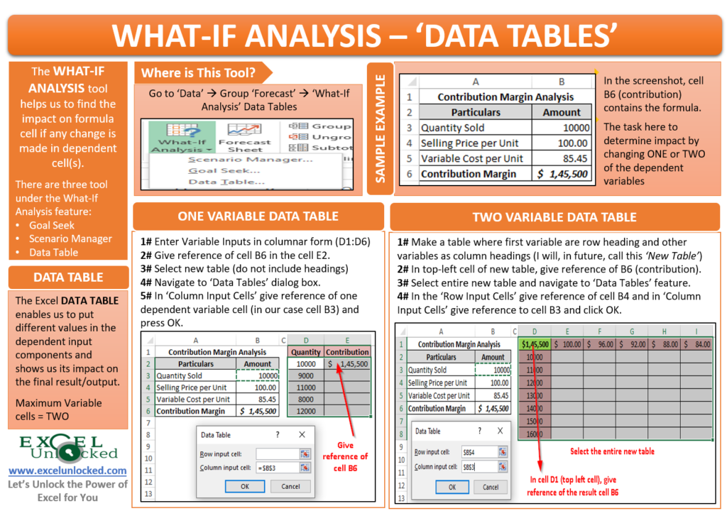
With a Data Table in Excel, you can easily vary one or two inputs and perform What-if analysis. A Data Table is a range of cells in which you can change values in some of the cells and come up with different answers to a problem.

There are two types of Data Tables −

One-variable Data Tables
Two-variable Data Tables

If you have more than two variables in your analysis problem, you need to use Scenario Manager Tool of Excel. For details, refer to the chapter – What-If Analysis with Scenario Manager in this tutorial.

One-variable Data Tables

A one-variable Data Table can be used if you want to see how different values of one variable in one or more formulas will change the results of those formulas. In other words, with a one-variable Data Table, you can determine how changing one input changes any number of outputs. You will understand this with the help of an example.

Example

There is a loan of 5,000,000 for a tenure of 30 years. You want to know the monthly payments (EMI) for varied interest rates. You also might be interested in knowing the amount of interest and Principal that is paid in the second year.

Analysis with One-variable Data Table

Analysis with one-variable Data Table needs to be done in three steps −

Step 1 − Set the required background.

Step 2 − Create the Data Table.

Step 3 − Perform the Analysis.

Let us understand these steps in detail −

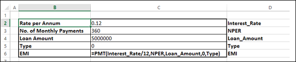
Step 1: Set the required background

Assume that the interest rate is 12%.
List all the required values.
Name the cells containing the values, so that the formulas will have names instead of cell references.
Set the calculations for EMI, Cumulative Interest and Cumulative Principal with the Excel functions – PMT, CUMIPMT and CUMPRINC respectively.

Your worksheet should look as follows −

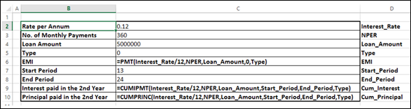
You can see that the cells in column C are named as given in the corresponding cells in column D.

Step 2: Create the Data Table

Type the list of values i.e. interest rates that you want to substitute in the input cell down the column E as follows −

As you observe, there is an empty row above the Interest Rate values. This row is for the formulas that you want to use.

Type the first function (PMT) in the cell one row above and one cell to the right of the column of values. Type the other functions (CUMIPMT and CUMPRINC) in the cells to the right of the first function.

Now, the two rows above the Interest Rate values look as follows −

The Data Table looks as given below −

Step 3: Do the analysis with the What-If Analysis Data Table Tool

Select the range of cells that contains the formulas and values that you want to substitute, i.e. select the range – E2:H13.
Click the DATA tab on the Ribbon.
Click What-if Analysis in the Data Tools group.
Select Data Table in the dropdown list.

Data Table dialog box appears.

Click the icon in the Column input cell box.
Click the cell Interest_Rate, which is C2.

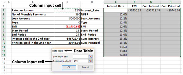
You can see that the Column input cell is taken as $C$2. Click OK.

The Data Table is filled with the calculated results for each of the input values as shown below −

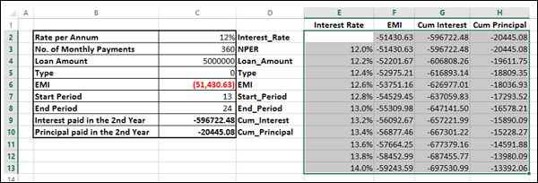
If you can pay an EMI of 54,000, you can observe that the interest rate of 12.6% is suitable for you.

Two-variable Data Tables

A two-variable Data Table can be used if you want to see how different values of two variables in a formula will change the results of that formula. In other words, with a twovariable Data Table, you can determine how changing two inputs changes a single output. You will understand this with the help of an example.

Example

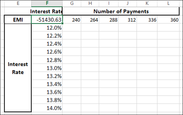
There is a loan of 50,000,000. You want to know how different combinations of interest rates and loan tenures will affect the monthly payment (EMI).

Analysis with Two-variable Data Table

Analysis with two-variable Data Table needs to be done in three steps −

Step 1 − Set the required background.

Step 2 − Create the Data Table.

Step 3 − Perform the Analysis.

Step 1: Set the required background

Assume that the interest rate is 12%.
List all the required values.
Name the cells containing the values, so that the formula will have names instead of cell references.
Set the calculation for EMI with the Excel function – PMT.

Your worksheet should look as follows −

You can see that the cells in the column C are named as given in the corresponding cells in the column D.

Step 2: Create the Data Table

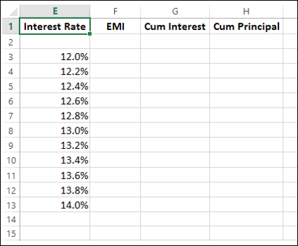
Type =EMI in cell F2.

Set EMI

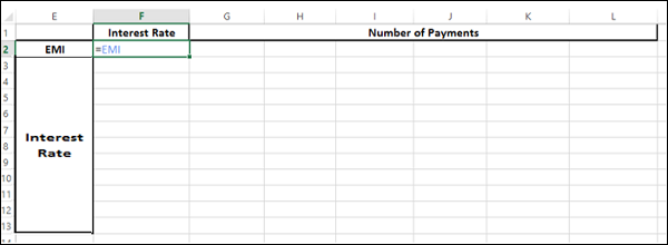
Type the first list of input values, i.e. interest rates down the column F, starting with the cell below the formula, i.e. F3.
Type the second list of input values, i.e. number of payments across row 2, starting with the cell to the right of the formula, i.e. G2.

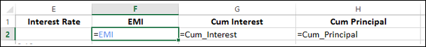
The Data Table looks as follows −

Do the analysis with the What-If Analysis Tool Data Table

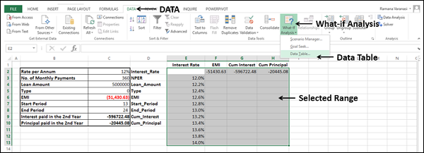
Select the range of cells that contains the formula and the two sets of values that you want to substitute, i.e. select the range – F2:L13.
Click the DATA tab on the Ribbon.
Click What-if Analysis in the Data Tools group.
Select Data Table from the dropdown list.

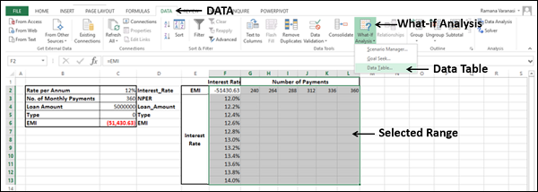
Data Table dialog box appears.

Click the icon in the Row input cell box.
Click the cell NPER, which is C3.
Again, click the icon in the Row input cell box.
Next, click the icon in the Column input cell box.
Click the cell Interest_Rate, which is C2.
Again, click the icon in the Column input cell box.

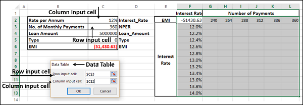
You will see that the Row input cell is taken as $C$3 and the Column input cell is taken as $C$2. Click OK.

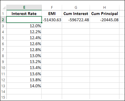
The Data Table gets filled with the calculated results for each combination of the two input values −

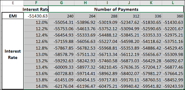
If you can pay an EMI of 54,000, the interest rate of 12.2% and 288 EMIs are suitable for you. This means the tenure of the loan would be 24 years.

Data Table Calculations

Data Tables are recalculated each time the worksheet containing them is recalculated, even if they have not changed. To speed up the calculations in a worksheet that contains a Data Table, you need to change the calculation options to Automatically Recalculate the worksheet but not the Data Tables, as given in the next section.

Speeding up the Calculations in a Worksheet

You can speed up the calculations in a worksheet containing Data Tables in two ways −

From Excel Options.
From the Ribbon.

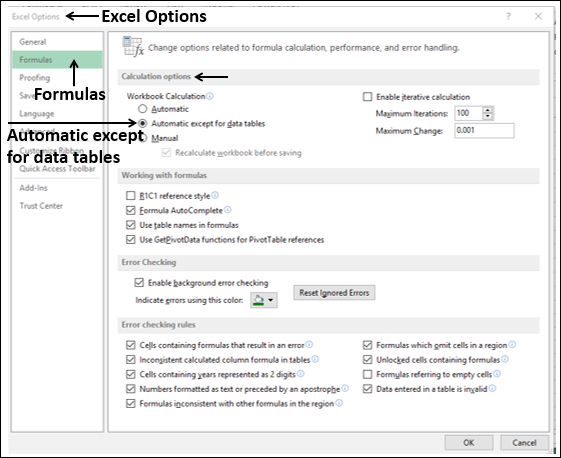
From Excel Options

Click the FILE tab on the Ribbon.
Select Options from the list in the left pane.

Excel Options dialog box appears.

From the left pane, select Formulas.
Select the option Automatic except for data tables under Workbook Calculation in the Calculation options section. Click OK.

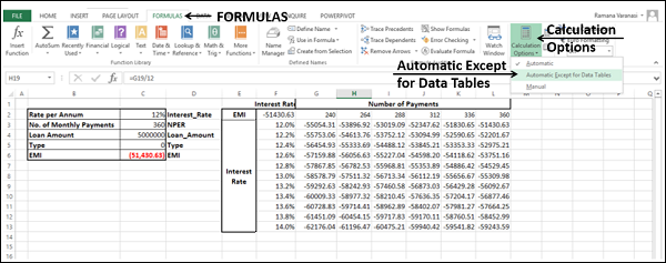
From the Ribbon

Click the FORMULAS tab on the Ribbon.
Click the Calculation Options in the Calculations group.
Select Automatic Except for Data Tables in the dropdown list.

Источник

Excel for Microsoft 365 Excel for Microsoft 365 for Mac Excel 2021 Excel 2021 for Mac Excel 2019 Excel 2019 for Mac Excel 2016 Excel 2016 for Mac Excel 2013 Excel 2010 Excel 2007 Excel for Mac 2011 More…Less

By using What-If Analysis tools in Excel, you can use several different sets of values in one or more formulas to explore all the various results.

For example, you can do What-If Analysis to build two budgets that each assumes a certain level of revenue. Or, you can specify a result that you want a formula to produce, and then determine what sets of values will produce that result. Excel provides several different tools to help you perform the type of analysis that fits your needs.

Note that this is just an overview of those tools. There are links to help topics for each one specifically.

What-If Analysis is the process of changing the values in cells to see how those changes will affect the outcome of formulas on the worksheet.

Three kinds of What-If Analysis tools come with Excel: Scenarios, Goal Seek, and Data Tables. Scenarios and Data tables take sets of input values and determine possible results. A Data Table works with only one or two variables, but it can accept many different values for those variables. A Scenario can have multiple variables, but it can only accommodate up to 32 values. Goal Seek works differently from Scenarios and Data Tables in that it takes a result and determines possible input values that produce that result.

In addition to these three tools, you can install add-ins that help you perform What-If Analysis, such as the Solver add-in. The Solver add-in is similar to Goal Seek, but it can accommodate more variables. You can also create forecasts by using the fill handle and various commands that are built into Excel.

For more advanced models, you can use the Analysis ToolPak add-in.

A Scenario is a set of values that Excel saves and can substitute automatically in cells on a worksheet. You can create and save different groups of values on a worksheet and then switch to any of these new scenarios to view different results.

For example, suppose you have two budget scenarios: a worst case and a best case. You can use the Scenario Manager to create both scenarios on the same worksheet, and then switch between them. For each scenario, you specify the cells that change and the values to use for that scenario. When you switch between scenarios, the result cell changes to reflect the different changing cell values.

1. Changing cells

2. Result cell

1. Changing cells

2. Result cell

If several people have specific information in separate workbooks that you want to use in scenarios, you can collect those workbooks and merge their scenarios.

After you have created or gathered all the scenarios that you need, you can create a Scenario Summary Report that incorporates information from those scenarios. A scenario report displays all the scenario information in one table on a new worksheet.

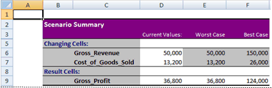
Note: Scenario reports are not automatically recalculated. If you change the values of a scenario, those changes will not show up in an existing summary report. Instead, you must create a new summary report.

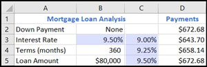
If you know the result that you want from a formula, but you’re not sure what input value the formula requires to get that result, you can use the Goal Seek feature. For example, suppose that you need to borrow some money. You know how much money you want, how long a period you want in which to pay off the loan, and how much you can afford to pay each month. You can use Goal Seek to determine what interest rate you must secure in order to meet your loan goal.

Cells B1, B2, and B3 are the values for the loan amount, term length, and interest rate.

Cell B4 displays the result of the formula =PMT(B3/12,B2,B1).

Note: Goal Seek works with only one variable input value. If you want to determine more than one input value, for example, the loan amount and the monthly payment amount for a loan, you should instead use the Solver add-in. For more information about the Solver add-in, see the section Prepare forecasts and advanced business models, and follow the links in the See Also section.

If you have a formula that uses one or two variables, or multiple formulas that all use one common variable, you can use a Data Table to see all the outcomes in one place. Using Data Tables makes it easy to examine a range of possibilities at a glance. Because you focus on only one or two variables, results are easy to read and share in tabular form. If automatic recalculation is enabled for the workbook, the data in Data Tables immediately recalculates; as a result, you always have fresh data.

Cell B3 contains the input value.
Cells C3, C4, and C5 are values Excel substitutes based on the value entered in B3.

A Data Table cannot accommodate more than two variables. If you want to analyze more than two variables, you can use Scenarios. Although it is limited to only one or two variables, a Data Table can use as many different variable values as you want. A Scenario can have a maximum of 32 different values, but you can create as many scenarios as you want.

If you want to prepare forecasts, you can use Excel to automatically generate future values that are based on existing data, or to automatically generate extrapolated values that are based on linear trend or growth trend calculations.

You can fill in a series of values that fit a simple linear trend or an exponential growth trend by using the fill handle or the Series command. To extend complex and nonlinear data, you can use worksheet functions or the regression analysis tool in the Analysis ToolPak Add-in.

Although Goal Seek can accommodate only one variable, you can project backward for more variables by using the Solver add-in. By using Solver, you can find an optimal value for a formula in one cell—called the target cell—on a worksheet.

Solver works with a group of cells that are related to the formula in the target cell. Solver adjusts the values in the changing cells that you specify—called the adjustable cells—to produce the result that you specify from the target cell formula. You can apply constraints to restrict the values that Solver can use in the model, and the constraints can refer to other cells that affect the target cell formula.

Need more help?

You can always ask an expert in the Excel Tech Community or get support in the Answers community.

Tools of what-if analysis

There are three tools in what-if analysis:

Goal seek
Scenario manager
Data Table

Goal seek

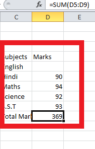
In goal seek we already know our output value we have to find the correct input value. For example, if a student wants to know his English marks and he knows all the rest of the marks and total marks in all subjects.

Step 1: Write all subjects and their marks in an excel sheet and do the sum by applying the formula sum.

Step 2: Go into the data tab of the Toolbar.

Step 3: Under the Data Table section, Select the What-if analysis.

Step 4: A drop-down appears. Select the Goal Seek.

Step 5: The dialogue box appears in the first column write the name of the cell in which you apply the formula sum. Type D10 in Set cell.

Step 6: In the second column write the value of the target. The target value for this example is 440.

Step 7: In the third column write the name of the cell in which you want to get marks in English. Provide absolute cell reference, i.e. $D$5.

Step 8: Click ok and see the result. The estimated marks for English are 71.

Scenario Manager

In scenario manager, we create different scenarios by proving different input values for the same variable than by comparing scenarios to choose the correct result. For Example, To check the cost of revenue for three different months.

Step 1: Given a data set, for Revenue Cost of Jan, with Expenses and Cost as its columns.

Step 2: Select the numerical value cell and Go to the Data.

Step 3: Under the forecast section, click on the What-if analysis.

Step 4: A drop-down appears. Select the Scenario manager.

Step 5: A dialog box appears in the dialog box select add option.

Step 6: A new dialog appears to write the name of the new scenario in the first column. Under Scenario name, write “Revenue of Feb”.

Step 7: In the second column select the changing cell. The changing cells for this example, are $E$5:$E$9.

Step 8: A new dialogue box name Scenario Values appears to write the changed value in the box. Enter the values as per shown in the image. Click Ok.

Step 9: Repeat step5, step6, and step8.

Step 10: Click Ok then select summary.

Step 11: A new Dialog box name Scenario Summary appears. Select Result cells: $E$10.

Step 12: See the result.

Data Table

In data, we create a table with different input values for the same variables. It is one of the most helpful features in what-if analysis. One can change different values in x and can achieve different outputs accordingly for research as well as business-driven purposes.

A data table is of two types:

Data table in one Variable

In the data table in one variable, we can change only one input value either in a row or in a column. It includes only one input cell. For example, a company wants to know about its revenue by changing the cost of raw materials by using a data table. Given a data set, with material and their cost.

Step 1: Create a table of revenue cost.

Step 2: Copy the last cell in which you get output in another cell. D7 for this example.

Step 3: Write the values in the cell for which you want to make a change in a column or in rows.

Step 4: Go to the data tab of the Toolbar.

Step 5: Under the data table section, Select the what-if analysis.

Step 6: A drop-down appears. Select the Data Table.

Step 7: A dialogue box name data table appears then select the cell in which you want to change the input value in a row or in the column. Input the value of the Column input cell to be $D$3. Click Ok. Your data table is ready.

Data table in two Variable

In the Data table in two variables, we can change two input values in both row and column. It includes two input cells. For example, A person wants to know about per month installments of loan by the different rates of interest and for the different time periods for the same principal amount.

Step 1: Create a table to find PMT.

Step 2: Copy the last cell in which you get output in another cell

Step 3: Write both values you want to change in both columns and rows.

Step 4: Go to the Data tab of the toolbar.

Step 5: Select the what-if analysis.

Step 6: Select the Data Table.

Step 7: A dialogue box appears in which you have to select the cell in which you want to change the value in both row and column. The Row input cell value is $D$5 and the column input cell value is $D$6.

Step 8: Click ok and see the result.

Источник

In our previous blogs, we learned about two of the What-If Analysis features in Excel – Goal Seek and Scenario Manager. In this blog, we would unlock the third and the last tool called Data Table Feature of Excel What-If Analysis. Like the other two, this feature also enables us to make the forecast. The Data Table What-If Analysis excel feature assists us to determine the impact on the result if any change is made in the dependent variable components.

Let us take one simple example to understand this functionality.

Table of Contents

Data Table – Example
Basics About Excel Data Table
Where Would You Find This Feature?
Creating a One-Variable Data Table
Creating A Two-Variable Data Table
How to Delete A Table

Data Table – Example

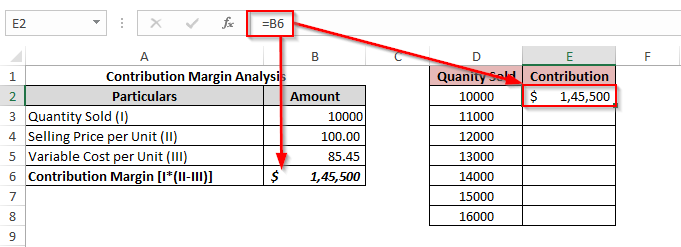
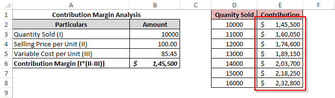
You are in the forecast and budgeting department in an organization and you use Excel as a utility software for performing your tasks. You are in the current in the process of preparing the contribution analysis budgeting tool for your manager’s usage.

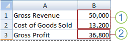
Below is the screenshot of the current quarter’s contribution margin.

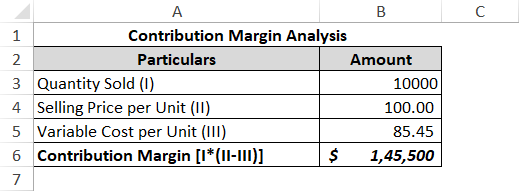
Contribution Margin AnalyContribution Margin Analysis Sample Datasis Sample Data

As you can see that the contribution margin (cell B6) contains the formula and is dependent on the other three variables (viz. Quantity sold, selling price, and variable cost per unit). The contribution margin is what is the final result and the other three are called the dependent variable components.

Now, suppose you want to analyze how the change in the dependent variables impact the contribution margin. You can perform the same by either using the Scenario Manager tool or the data table feature. The scenario manager feature has already been covered in our previous blog.

In this blog, we would learn to use the data table to achieve the desired objective.

Basics About Excel Data Table

Just like the other two What-If Analysis Tools, the Excel Data table feature also helps us to do forecasting. It enables us to put different values in the dependent input components and shows us its impact on the final result/output.

The example provided in the above section is a simple one, just to make you understand the functionality. You can use the what-if analysis tools with complex formula structure for your performing the budgeting/forecasting.

Unlike the scenario manager tool, where you can create scenarios with 32 variable components, the data table can be used when you want to analyze the impact on the formula cell by changing a maximum up to TWO variable components.

In the upcoming sections of this blog, you would learn both – one variable and two variables data table creation and many more related functions.

It is important to note that the ‘Data Table’ should not be confused with ‘Excel Tables’. Excel Tables are normal tables with few additional advantages.

Let us now begin.

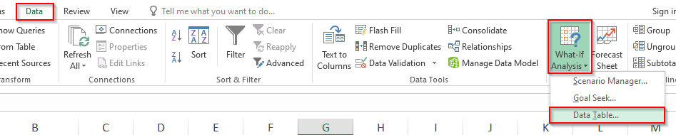
Where Would You Find This Feature?

Navigate to the following path to reach to this tool: Data tab > Forecast Tool > What-If Analysis button > Data Table.

Creating a One-Variable Data Table

The one variable data table allows you to see the impact on the result cell by changing one of the variable input cells.

Follow the below steps:

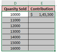
Enter the variable input values for which you want to do result analysis in either column or row. Firstly, we would learn to create a data table using the column-oriented tool. Therefore, I have put the variable input values in the form of a column.

In the adjacent cell, we want to have the resultant contribution amount. So, give the reference of the cell B6 in this adjacent cell.

Refer to the screenshot below:

Now, select the data range including all the cells except the heading cells (in our example range D2:E8)

Navigate to the Data Table tool (as shown in the above section), and the ‘Data Table’ dialog box would pop out on your screen.

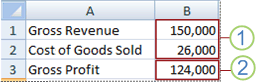
Now, click on the ‘Column Input Cell’ (As the quantities sold are in a column form) and give reference to the cell B3 in the original table. Cell B3 represents the variable Quantity Sold.

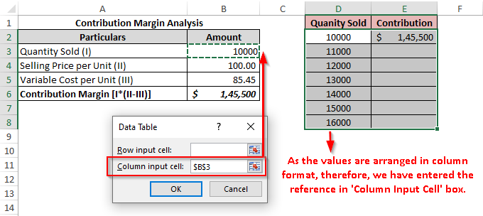
Finally, click on the ‘OK’ button and as a result, you would notice that the excel fills the contribution column (Column E) with the contribution amount based on the formula.

You can even arrange the resultant table in the row orientation. In that case, the only change is that you need to enter the reference formula in ‘Row Input Cell’ instead of the ‘Column Input Cell’.

Refer to the below screenshot:

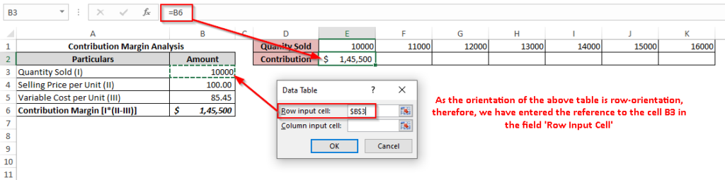
The result would be as under:

Creating A Two-Variable Data Table

The two-variable data table helps to determine the change in the formula cell when two dependent variables change simultaneously.

In the same example, let us understand the impact on the contribution with a simultaneous change in the quantity sold and selling price per unit, keeping the variable cost per unit as a constant value of $85.45 per unit.

Follow the below steps to achieve the same:

Where you want to create a two-variable data table, you need to put one variable as the table row and another as the table columns.

I have put the column headings as the quantity sold and row headings are selling price per unit.

Then give reference to the contribution margin cell from the original table (cell B6) in this top-left cell of this newly created table as highlighted in the screenshot below:

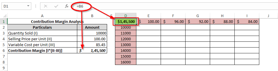
Firstly, select the entire table from D1 to I8 and then open the ‘Data Table’ dialog box.

In the section, ‘Row Input Cell’ select the cell B4 from the original table. This represents the row heading in the newly created table). Similarly, in section, ‘Column Input Cell’, select cell B3 from the original table, which represents the column headings in the new table.

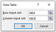
As soon as you click on the ‘OK’ button, you would notice that the excel fills the blank cell s in this newly created table with the appropriate values. Refer to the screenshot below:

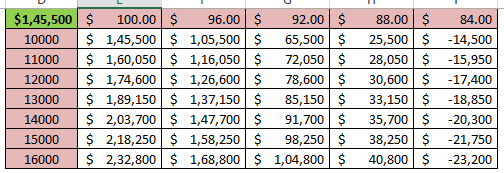
Therefore, we can see that if we sell 14,000 units at $96 each, then we would earn a contribution margin of $ 1,47,700.

This brings us to the end of this section.

How to Delete A Table

Before starting with deleting the data table, let us perform one activity. Select a cell in the data table then use your keyboard and press the ‘Delete’ key.

What did you notice? Did the excel allow you to delete the individual cell value in the data table?

The answer is NO !!

The Excel pops out a message dialog box. Refer to the screenshot below:

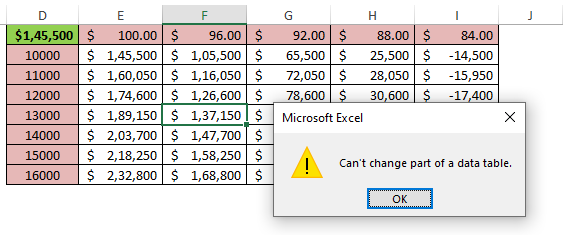
However, when you would try to delete the entire table, the excel would allow. Just, select the entire table and use your keyboard to ‘Delete’.

As a result, Excel would allow you to delete the values.

This brings us to the end of this blog. Share your views and comments in the comment section below.

How to Add Conditional Column in Excel Power Query
Introduction to Charts in Microsoft Excel
Making Calculated Field in Pivot Table in Excel
How to Make A Table In Excel – A Hidden Functionality
Quick Overview On Pivot Table in Excel
Pivot Table in Excel – Making Pivot Tables

Источник

The Dataset

The Set Up

Data Table Example

Limitations

Conclusion

One-variable Data Tables

Analysis with One-variable Data Table

Step 1: Set the required background

Step 2: Create the Data Table

Step 3: Do the analysis with the What-If Analysis Data Table Tool

Two-variable Data Tables

Analysis with Two-variable Data Table

Step 1: Set the required background

Step 2: Create the Data Table

Do the analysis with the What-If Analysis Tool Data Table

Data Table Calculations

Speeding up the Calculations in a Worksheet

From Excel Options

From the Ribbon

Need more help?

See Also

Need more help?

What is What-if Analysis?

Tools of what-if analysis

Goal seek

Scenario Manager

Data Table

Data Table – Example

Basics About Excel Data Table

Where Would You Find This Feature?

Creating a One-Variable Data Table

Creating A Two-Variable Data Table

How to Delete A Table

RELATED POSTS