
On this webpage I discuss a number of problems with data tables, and how to repair the problems using simple VBA programs. I demonstrate that relatively simple and short VBA code can be used as an alternative to data tables that the problems. The main principle when using the VBA alternative to data tables is using a FOR and NEXT loop along with the CELLS tool. You can quickly make a one-way or a two-way data table by going around and changing a row or a column cell in the loop and then using the same loop to show the output. You can make the VBA code very flexible so that it can start on different rows and different columns. When making the code flexible, you can use the .ROW and .COLUMN things in VBA (I don’t know the official name) along with .ROWS.COUNT and .COLUMNS.COUNT. You can also make the code flexible so you can use alternative range names for inputs and outputs. The VBA method to make data tables is also a good way work through the fundamental ideas of creating VBA programs. So, on this page I present two different methods to program the data tables. The first method that I present is using an output range and deriving the rows and columns from the range name. The second method uses definitions of row start and row end along with a FOR and NEXT loop.
Instructions for Downloading Files with Macros
.
Some Problems with the Excel Data Table Tool
When you use VBA code instead of data tables you can fix many of the problems. You can illustrate the scenario analysis with a graph because you don’t have to fill in the blank with a number. If you have a big database file while your little file with a data table is open (even with the calculation method adjusted). This will slow things down a lot. Say you do not want to use code numbers but you want to put your sensitivity analysis in another sheet. You will be stuck. If you have a goal seek and would like to make your sensitivity analysis work with the goal seek you will also be frustrated. You can use a crude and unflexible method with row numbers and column number input as illustrated below. In this case, a data table is made with a copy and paste routine.
Sub table2()

For Row = 72 To 74
      Range("leverage1").Value = Cells(Row, 6).Value
       For col = 7 To 9
            Range("idc_1").Value = Cells(71, col)
            copy_paste_fee
            Cells(Row, col).Value = Range("debt1")
        Next col
Next Row

End Sub
VBA code can fix problem with data tables. These problems involve writing a macro that should take two minutes:
- Inputs for the data table must be in same sheet as the data table itself. This is fixed by using range names and changing the inputs with the CELLS function.
- Data tables slow you down when save and open even if using automatic except data tables calculation option is selected
- When you press the F9 to re-calculate, you can mess things up even if you have a large data table
- Because of the restricted formatting when you make a data table, you cannot easily make a graph with the F11 key.
- You cannot use the goal seek with a data table where excel would somehow magically know to run the goal seek function every time the sensitivity tables are run.
- It can be a pain to put the input variables in different sheets when do not use code numbers.
- Data tables cannot be used with copy and paste macros (they can be used with the UDF method).
The code below is for a one way data table that uses the range name OUTPUT. Note how you can create a lot just from the range name using the .ROWS.count. In this case, a scenario number is being used to drive the results and the results are in a single line.
Sub One_Way_Table()

total_rows = Range("output").Rows.Count
total_cols = Range("output").Columns.Count

    For Row = 1 To total_rows

       Range("scenario").Value = Row

       For col = 1 To total_cols
           Range("output").Cells(Row, col).Value = Range("results").Cells(1, col).Value
       Next col

    Next Row

End Sub
Output Range Method of Computing Data Tables
In my revised method, I simply define a range named output that is a square with rows and columns. You can use this square to find the number of rows and columns as well as the starting row and the starting column. You can use the total rows and the total columns in the FOR and NEXT loop and you can also use the starting row and the starting column to create sensitivity ranges for the data table. You can download the file with VBA code by clicking on the button below. The screenshot below the button demonstrates the output of the data table. The key things to add to your VBA include:
The code below is for a two way data table. It includes some colouring and other items. Here the start row and the end row and the start colum and end colum are used with the .ROW and .ROWS,COUNT.
Sub table5()

Range("output1").Clear
Range("output1").Interior.Color = 60000

row_start = Range("output1").Row
row_end = row_start + Range("output1").Rows.Count - 1
col_start = Range("output1").Column
col_end = col_start + Range("output1").Columns.Count - 1

For Row = row_start To row_end

   Range("leverage1").Value = Cells(Row, col_start - 1).Value

   For col = col_start To col_end
     Range("idc_1").Value = Cells(row_start - 1, col)
     copy_paste_fee Cells(Row, col).Value = Range("debt1")
   Next col
Next Row
End Sub
.
.
| rows = range(“output”).rows.count |
| columns = range(“output”).columns.count |
| row_start = range(“ouptut”).row |
| col_start = range(“output”).col |
| row_sensitivity = row_start – 1 |
| col_sensitivity = col_start – 1 |
.
Excel File with VBA Code for Creating a Data Table from the an Output Range with Efficiency Tests
.
.
.
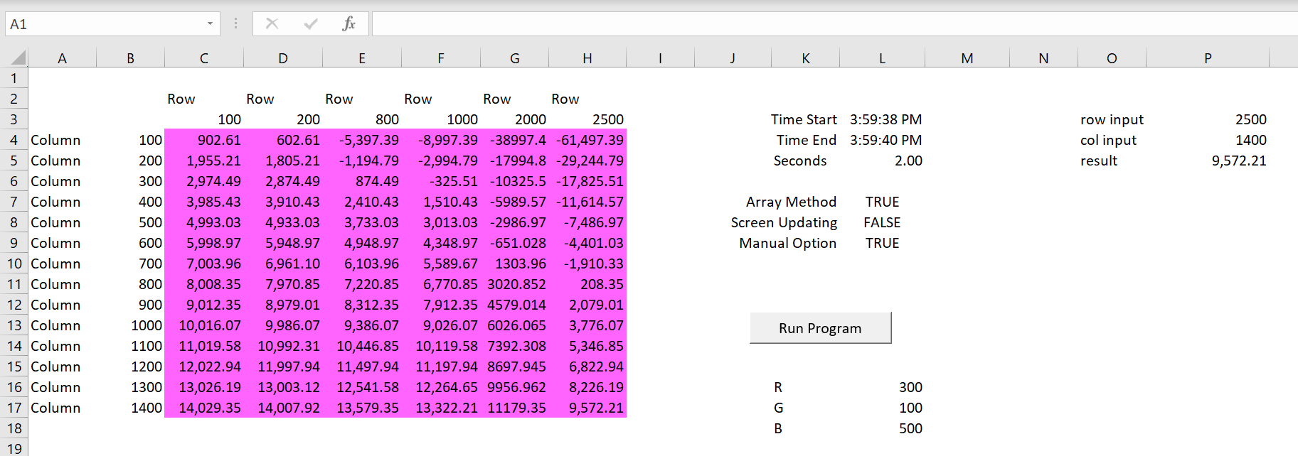
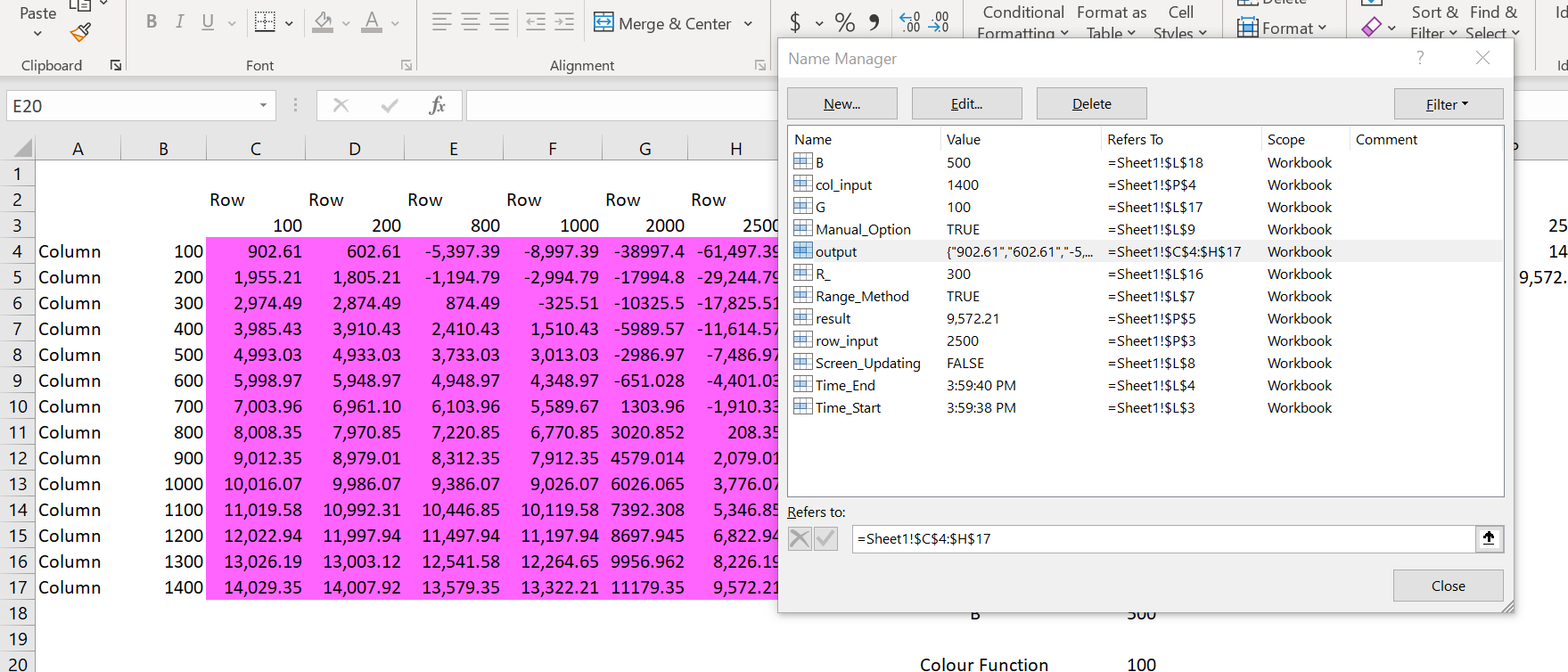
The method works by creating a range name that is illustrated on the screenshot below. You can use CNTL, F3 to change the dimensions of the range name and the data table will change as hopefully shown on the screenshot. This changes the dimension of the FOR and NEXT loop from the range(“output”).rows.count and the range(“output”).columns.count. The VBA code is shown at the bottom of this section.
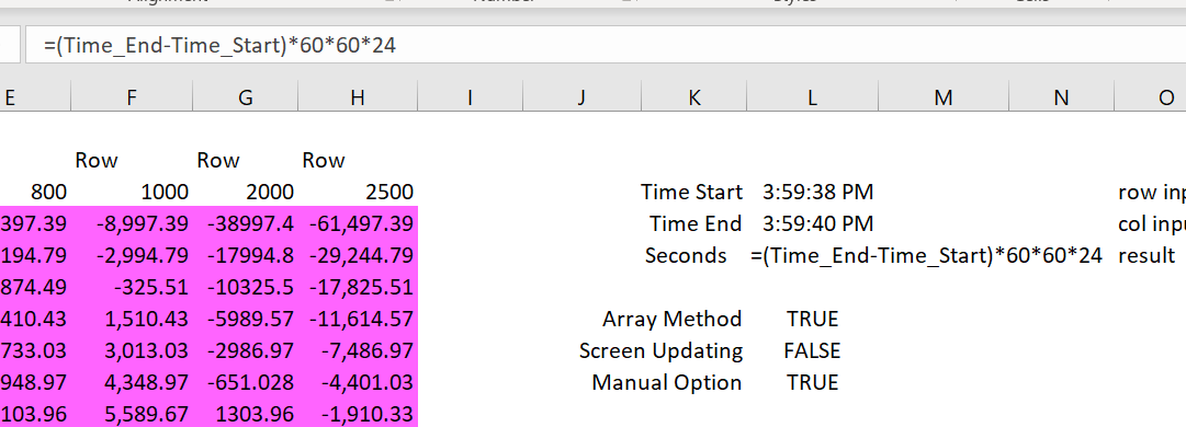
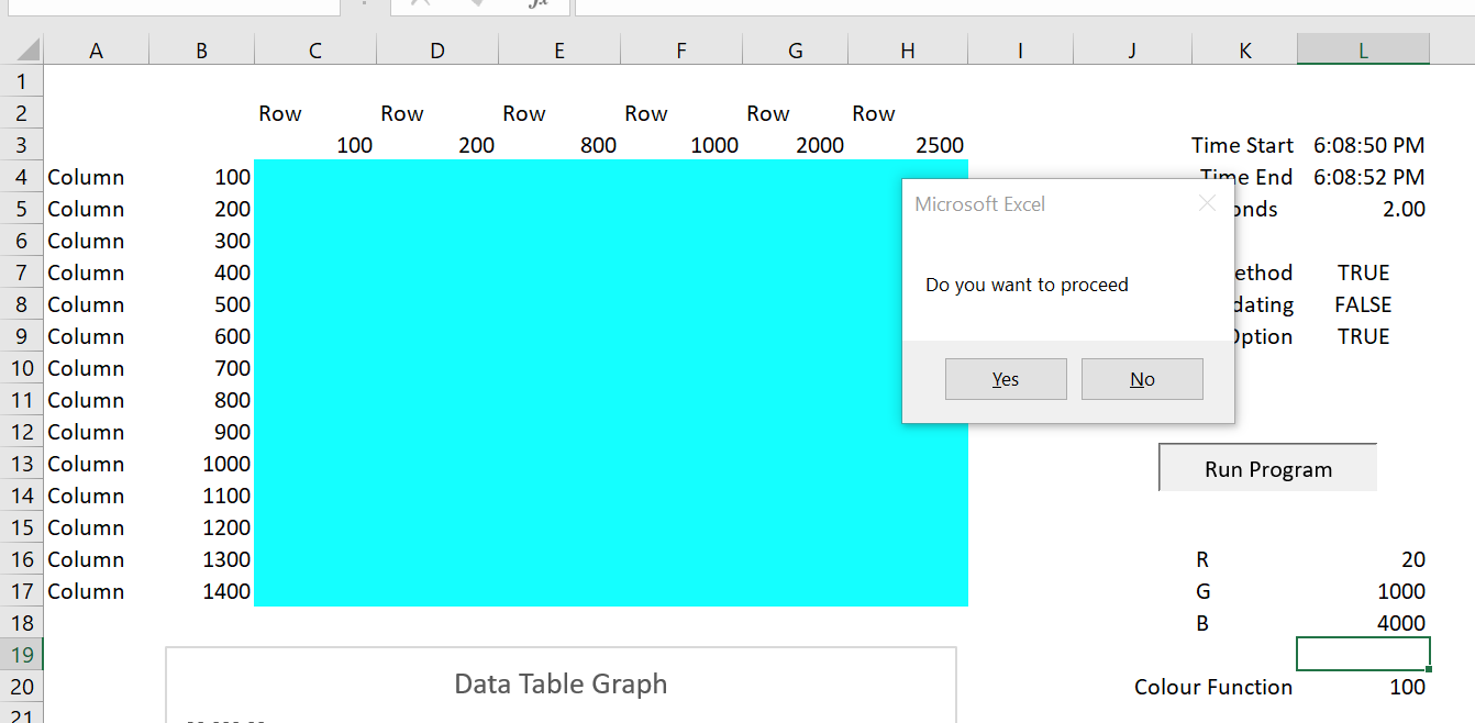
In testing alternative VBA code including only re-calculating the calculation of calculated cell; using the application.screenupdating =false and using an array variable rather than directly writing to the output variable. In evaluating the alternative strategies I have printed the length of time it takes to run the loop. The manner in which the time can be converted to seconds is illustrated in the screenshot below. To present the time, you can use the Range(“Start_time”) = time before the loop and the statement Range(“End_time”) = time after the loop. This is illustrated in the screenshot below.
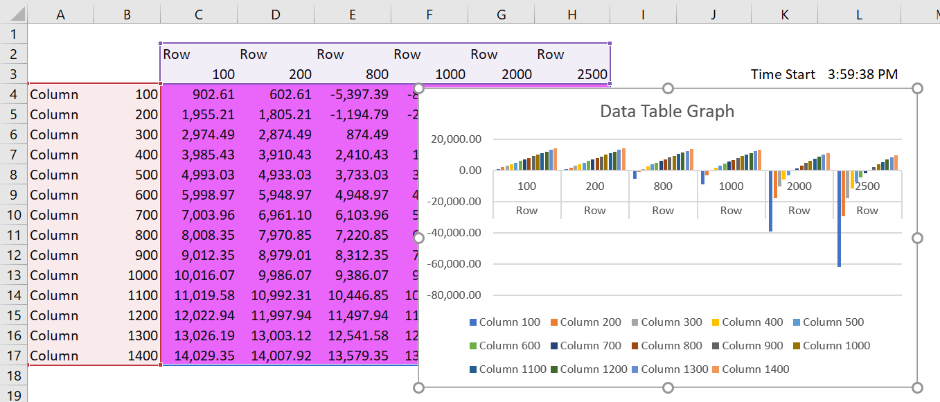
The screenshot below illustrates how you can make a graph from the data table. This is not possible with the normal data table because of the formula between the row and the column. Remember that the row and the column title must be blank for the x-axis to be used.
The screenshot below illustrates how you can change the colour of the output range with the code range(“output”) = RGB( red number, green number, blue number). In this case the red, green and blue codes are read in from the excel sheet. The code for this is shown in the VBA code below.
.
testSub table()
' When you change to manual and define the calculation area you can speed up a lot
current_status = Application.Calculation
' Get the current calcluation methodIf Range("Manual_option") Then Application.Calculation = xlCalculationManual
' Change to manual
Application.ScreenUpdating = True
' To show the cleared areaMsgBox " Before clear "
' Standard mgsboxRange("output").ClearContents
' Clear out the rangeApplication.ScreenUpdating = False
If Range("screen_updating") Then Application.ScreenUpdating = Truerange_method = Range("range_method")
' read the true or false from the sheetDim result() As Variant
' sets-up a flexibe array variabletest = MsgBox(" Do you want to proceed ", vbYesNo)
' put a question in msgboxIf test <> 6 Then Exit Sub
' exit the sub if not equal to 6=trueRange("output").Interior.Color = RGB(Range("R_"), Range("G"), Range("B"))
' try the RGB with the outputTotal_Rows = Range("output").Rows.Count
' Use the .rows to find the total rowsTotal_Columns = Range("output").Columns.Count
' Use the .columns to find the total rowsReDim result(Total_Rows, Total_Columns)
' Used for the range methodstart_row = Range("output").Row
' The start row for the range namestart_col = Range("output").Column
' The start columnRange("time_start") = Time
' put the start time in the sheetFor Row = 1 To Total_Rows
' Start of nested loopRange("col_input") = Cells(Row + start_row - 1, start_col - 1)
' Key -- define the column inputFor col = 1 To Total_Columns
' loop around columnsRange("row_input") = Cells(start_row - 1, col + start_col - 1) ' Go around columns and set the row input
Range("result").Calculate
' Only calculates the output cell -- the key to making the model work fastIf range_method = False Then Range("output").Cells(Row, col) = Range("result") ' Simple methood
If range_method = True Then result(Row, col) = Range("result") ' Puts output into an array to make faster
Next col
Next Row
If range_method = True Then Range("output") = result
' If put into array, fill up output with valueRange("time_end") = Time
Application.Calculation = current_status
' Reset the calculuation method to the originalEnd Sub
Data Table using Prior Method with Row Start, Row End, Column Start, and Column End
I have made a simple file that demonstrates how to make multiple data tables and solve the problems with data tables in excel. This file includes the VBA code that is demonstrated in the video below and creates four different flexible data tables from the valuation analysis.
Excel File with Simple Valuation Model that Illustrates VBA Principles that you can use to make Multiple Data Tables
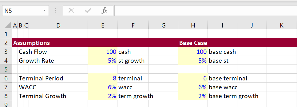
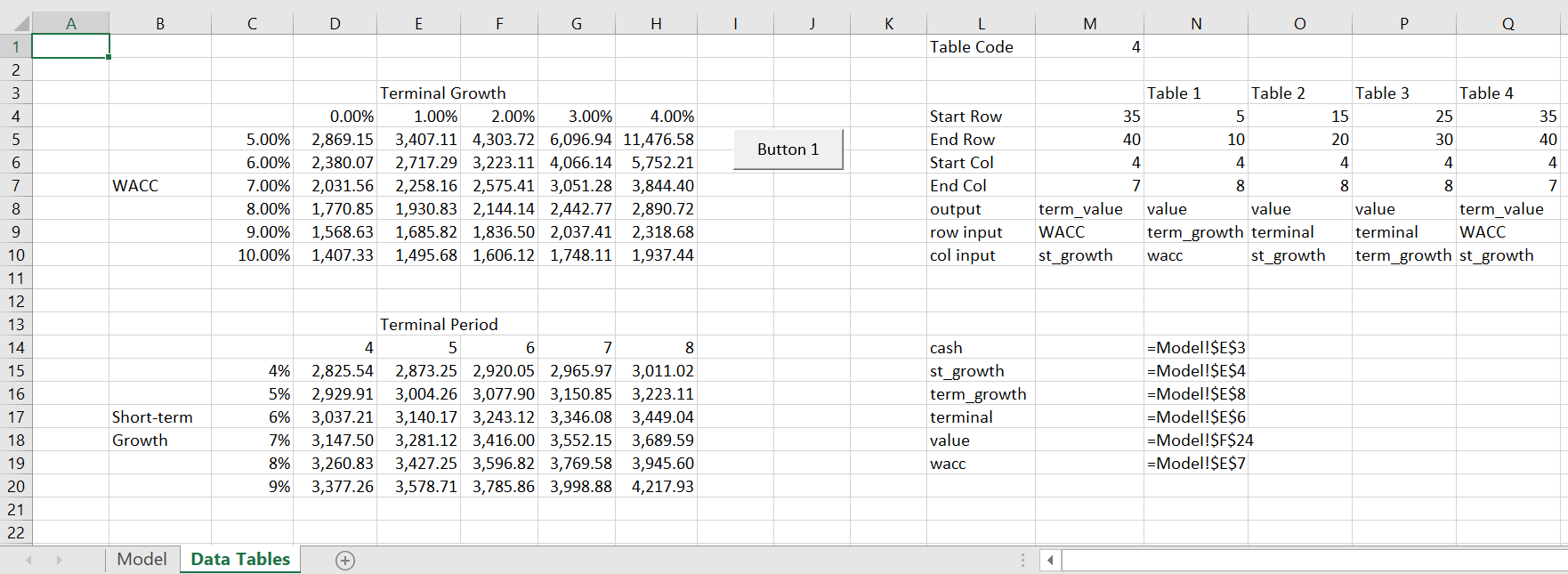
I am using the case of building data tables with VBA to demonstrate some VBA principles of FOR/NEXT and using VBA with the INDEX function in excel. In the exercise, I use a very simple valuation example where we want to investigate the effect of WACC, Terminal Growth, Short-term Growth and the length of the explicit period. The screenshot below illustrates the inputs. Note that I put names next to the inputs and I used the SHIFT, CNTL, F3 keystrokes to make named ranges. I also put the base case values with range names next to the values that are used in the model. The range names are important because they are used in the VBA code.
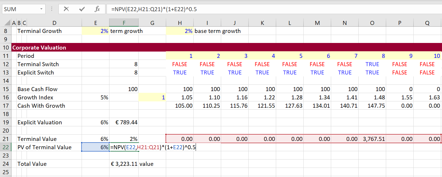
The second screenshot demonstrates the model with outputs that will be used in the data tables. Note that I put a name next to the total value and next to the terminal value which will be outputs of a series of data tables. The model allows you to use alternative terminal value dates and includes a half-year convention. I pretend that you want a whole lot of data tables with different explicit periods; different short-term growth rates as well as the WACC and the terminal growth which are in almost every sensitivity table.
Now let’s move to creation of the data tables in a new sheet. The data tables will not have the irritating thing in the middle that prevents you from making graphs. The format of the graphs is shown in the screenshot below. Note that I have chosen different variables for the row and column input.
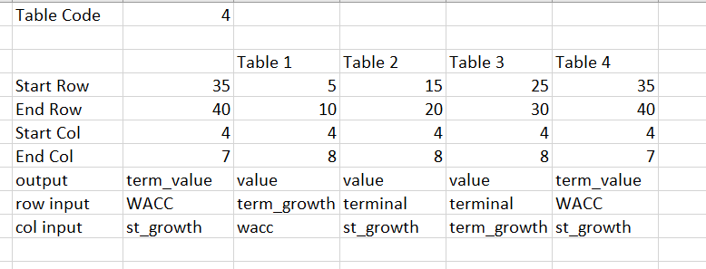
To make the data tables, define the row start, row end, column start and column end. Then also define the range names that will be used for the row input and column input. When entering the data, use in INDEX function so that you can choose alternative data tables. The VBA code will move through the different data tables by changing the code number. The values that are currently in use are in the left hand side of the table. As the data table 4 is in place, the start row is 35 and the start column is 40 and the output is the terminal value. You can make as many data tables as you want and this will work with by changing code number that is shown is 4 in the example below.
Now lets run the data table. This is done with VBA code that loops through the rows and columns of the data table defined from the range names shown in the screenshot above. The VBA code is illustrated at the bottom of this explanation.
The VBA code is shown below. There are two programs. The first program creates one data table with FOR/NEXT and the CELLS statements. You go up one row from the start row to define the series of row scenarios. You go one to the left to get the column scenarios associated with the column input. The code includes an error check and at the end of the data table I re-assigned the data to the base case.
.
Sub table()

'cash
'st_growth
'term_growth
'terminal
'Value
'wacc

For Row = Range("start_row") To Range("end_row")

Range(Range("col_input")) = Cells(Row, Range("start_col") - 1)

For col = Range("start_col") To Range("end_col")
Range(Range("row_input")) = Cells(Range("start_row") - 1, col)

On Error GoTo out_of_loop:
Cells(Row, col) = Range(Range("output"))

back_to_loop:

Next col
Next Row


'
' Reset the values to base case
'

Range("cash") = Range("Base_cash")
Range("st_growth") = Range("Base_st")
Range("term_growth") = Range("Base_terminal")
Range("wacc") = Range("Base_wacc")
Range("term_growth") = Range("base_term_growth")


Exit Sub

out_of_loop:

Resume back_to_loop:

End Sub

.
The second VBA code demonstrates how to create multiple data tables from this code. You define the code used in the INDEX excel function. Then you use a FOR/NEXT loop to change the index code number.
.
Sub all_tables()

For table_no = 1 To 4

Range("table_code") = table_no
table

Next table_no

End Sub

.
.
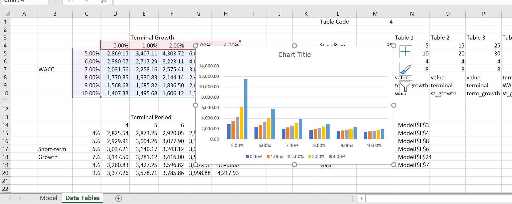
Graphs with Data Tables made by VBA
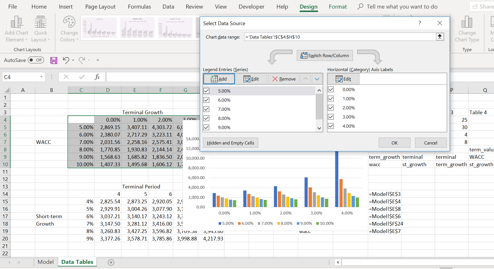
One of the things I really hate about data tables made with excel is that you cannot quickly make graphs because of the number at the top left of the table. With the VBA method you have much more flexibility. With the data tables created from the code shown in the associated file, you can select the area of the table including the row and column sensitivity variables. Then you can press F11 or press ALT and F9. This will create a graph that shows the inter-relationships between the variables. This is demonstrate in the screenshots below. The second screenshot shows how you can change the row and column variables by clicking on the select data thing.
Video Explanations
.
.
Speeding up Data Tables by Assigning the Output to a Range Name
Going around rows and columns can take some time. To speed things up you can assign the output to an array variable. This is demonstrated in the little test VBA code below.
.

Sub table()

Dim temp_out(9000, 1) As Single

num = Range("row_end") - Range("row_start") + 1

range_name = "P" & Range("row_start") & ":P" & Range("row_end")

num = 1

For Row = Range("row_start") To Range("row_end")

Range("gross_load") = Cells(Row, Range("column"))

temp_out(num, 1) = Range("total_cost_for_hour")

num = num + 1

Next Row

Range(range_name) = temp_out


End Sub


.
.
Tables are one of the most powerful features of Excel. Controlling them using VBA provides a way to automate that power, which generates a double benefit 🙂
Excel likes to store data within tables. The basic structural rules, such as (a) headings must be unique (b) only one header row allowed, make tables compatible with more complex tools. For example, Power Query, Power Pivot, and SharePoint lists all use tables as either a source or an output. Therefore, it is clearly Microsoft’s intention that we use tables.
However, the biggest benefit to the everyday Excel user is much simpler; if we add new data to the bottom of a table, any formulas referencing the table will automatically expand to include the new data.
Whether you love tables as much as I do or not, this post will help you automate them with VBA.
Tables, as we know them today, first appeared in Excel 2007. This was a replacement for the Lists functionality found in Excel 2003. From a VBA perspective, the document object model (DOM) did not change with the upgraded functionality. So, while we use the term ‘tables’ in Excel, they are still referred to as ListObjects within VBA.
Download the example file
I recommend you download the example file for this post. Then you’ll be able to work along with examples and see the solution in action, plus the file will be useful for future reference.
![]()
Download the file: 0009 VBA tables and ListObjects.zip
Structure of a table
Before we get deep into any VBA code, it’s useful to understand how tables are structured.
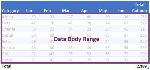
Range & Data Body Range
The range is the whole area of the table.
The data body range only includes the rows of data, it excludes the header and totals.
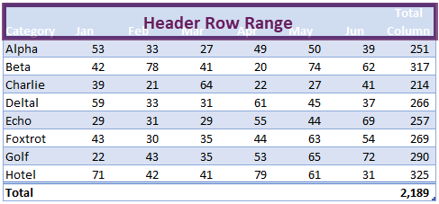
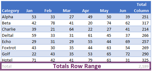
Header and total rows
The header row range is the top row of the table containing the column headers.
The totals row range, if displayed, includes calculations at the bottom of the table.
List columns and list rows
The individual columns are known as list columns.
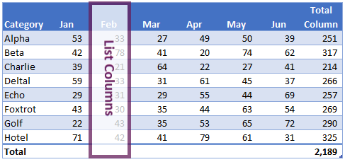
Each row is known as a list row.
The VBA code in this post details how to manage all these table objects.
Referencing the parts of a table
While you may be tempted to skip this section, I recommend you read it in full and work through the examples. Understanding Excel’s document object model is the key to reading and writing VBA code. Master this, and your ability to write your own VBA code will be much higher.
Many of the examples in this first section use the select method, this is to illustrate how to reference parts of the table. In reality, you would rarely use the select method.
Select the entire table
The following macro will select the whole table, including the totals and header rows.
Sub SelectTable()

ActiveSheet.ListObjects("myTable").Range.Select

End Sub
Select the data within a table
The DataBodyRange excludes the header and totals sections of the table.
Sub SelectTableData()

ActiveSheet.ListObjects("myTable").DataBodyRange.Select

End Sub
Get a value from an individual cell within a table
The following macro retrieves the table value from row 2, column 4, and displays it in a message box.
Sub GetValueFromTable()

MsgBox ActiveSheet.ListObjects("myTable").DataBodyRange(2, 4).value

End Sub
Select an entire column
The macro below shows how to select a column by its position, or by its name.
Sub SelectAnEntireColumn()

'Select column based on position
ActiveSheet.ListObjects("myTable").ListColumns(2).Range.Select

'Select column based on name
ActiveSheet.ListObjects("myTable").ListColumns("Category").Range.Select

End Sub
Select a column (data only)
This is similar to the macro above, but it uses the DataBodyRange to only select the data; it excludes the headers and totals.
Sub SelectColumnData()

'Select column data based on position
ActiveSheet.ListObjects("myTable").ListColumns(4).DataBodyRange.Select

'Select column data based on name
ActiveSheet.ListObjects("myTable").ListColumns("Category").DataBodyRange.Select

End Sub
Select a specific column header
This macro shows how to select the column header cell of the 5th column.
Sub SelectCellInHeader()

ActiveSheet.ListObjects("myTable").HeaderRowRange(5).Select

End Sub
Select a specific column within the totals section
This example demonstrates how to select the cell in the totals row of the 3rd column.
Sub SelectCellInTotal()

ActiveSheet.ListObjects("myTable").TotalsRowRange(3).Select

End Sub
Select an entire row of data
The macro below selects the 3rd row of data from the table.
NOTE – The header row is not included as a ListRow. Therefore, ListRows(3) is the 3rd row within the DataBodyRange, and not the 3rd row from the top of the table.
Sub SelectRowOfData()

ActiveSheet.ListObjects("myTable").ListRows(3).Range.Select

End Sub
Select the header row
The following macro selects the header section of the table.
Sub SelectHeaderSection()

ActiveSheet.ListObjects("myTable").HeaderRowRange.Select

End Sub
Select the totals row
To select the totals row of the table, use the following code.
Sub SelectTotalsSection()

ActiveSheet.ListObjects("myTable").TotalsRowRange.Select

End Sub
OK, now we know how to reference the parts of a table, it’s time to get into some more interesting examples.
Creating and converting tables
This section of macros focuses on creating and resizing tables.
Convert selection to a table
The macro below creates a table based on the currently selected region and names it as myTable. The range is referenced as Selection.CurrentRegion, but this can be substituted for any range object.
If you’re working along with the example file, this macro will trigger an error, as a table called myTable already exists in the workbook. A new table will still be created with a default name, but the VBA code will error at the renaming step.
Sub ConvertRangeToTable()

tableName As String
Dim tableRange As Range

Set tableName = "myTable"
Set tableRange = Selection.CurrentRegion
ActiveSheet.ListObjects.Add(SourceType:=xlSrcRange, _
    Source:=tableRange, _
    xlListObjectHasHeaders:=xlYes _
    ).Name = tableName

End Sub
Convert a table back to a range
This macro will convert a table back to a standard range.
Sub ConvertTableToRange()

ActiveSheet.ListObjects("myTable").Unlist

End Sub
NOTE – Unfortunately, when converting a table to a standard range, the table formatting is not removed. Therefore, the cells may still look like a table, even when they are not – that’s frustrating!!!
Resize the range of the table
To following macro resizes a table to cell A1 – J100.
Sub ResizeTableRange()

ActiveSheet.ListObjects("myTable").Resize Range("$A$1:$J$100")

End Sub
Table styles
There are many table formatting options, the most common of which are shown below.
Change the table style
Change the style of a table to an existing pre-defined style.
Sub ChangeTableStyle()

ActiveSheet.ListObjects("myTable").TableStyle = "TableStyleLight15"

End Sub
To apply different table styles, the easiest method is to use the macro recorder. The recorded VBA code will include the name of any styles you select.
Get the table style name
Use the following macro to get the name of the style already applied to a table.
Sub GetTableStyleName()

MsgBox ActiveSheet.ListObjects("myTable").TableStyle

End Sub
Apply a style to the first or last column
The first and last columns of a table can be formatted differently using the following macros.
Sub ColumnStyles()

'Apply special style to first column
ActiveSheet.ListObjects("myTable").ShowTableStyleFirstColumn = True

'Apply special style to last column
ActiveSheet.ListObjects("myTable").ShowTableStyleLastColumn = True

End Sub
Adding or removing stripes
By default, tables have banded rows, but there are other options for this, such as removing row banding or adding column banding.
Sub ChangeStripes()

'Apply column stripes
ActiveSheet.ListObjects("myTable").ShowTableStyleColumnStripes = True

'Remove row stripes
ActiveSheet.ListObjects("myTable").ShowTableStyleRowStripes = False

End Sub
Set the default table style
The following macro sets the default table style.
Sub SetDefaultTableStyle()

'Set default table style
ActiveWorkbook.DefaultTableStyle = "TableStyleMedium2"

End Sub
Looping through tables
The macros in this section loop through all the tables on the worksheet or workbook.
Loop through all tables on a worksheet
If we want to run a macro on every table of a worksheet, we must loop through the ListObjects collection.
Sub LoopThroughAllTablesWorksheet()

'Create variables to hold the worksheet and the table
Dim ws As Worksheet
Dim tbl As ListObject

Set ws = ActiveSheet
'Loop through each table in worksheet
For Each tbl In ws.ListObjects

    'Do something to the Table....

Next tbl

End Sub
In the code above, we have set the table to a variable, so we must refer to the table in the right way. In the section labeled ‘Do something to the table…, insert the action to be undertaken on each table, using tbl to reference the table.
For example, the following will change the table style of every table.
tbl.TableStyle = "TableStyleLight15"
Loop through all tables in a workbook
Rather than looping through a single worksheet, as shown above, the macro below loops through every table on every worksheet.
Sub LoopThroughAllTablesWorkbook()

'Create variables to hold the worksheet and the table
Dim ws As Worksheet
Dim tbl As ListObject

'Loop through each worksheet
For Each ws In ActiveWorkbook.Worksheets

    'Loop through each table in worksheet
    For Each tbl In ws.ListObjects

        'Do something to the Table....

    Next tbl

Next ws

End Sub
As noted in the section above, we must refer to the table using its variable. For example, the following will display the totals row for every table.
tbl.ShowTotals = True
Adding & removing rows and columns
The following macros add and remove rows, headers, and totals from a table.
Add columns into a table
The following macro adds a column to a table.
Sub AddColumnToTable()

'Add column at the end
ActiveSheet.ListObjects("myTable").ListColumns.Add

'Add column at position 2
ActiveSheet.ListObjects("myTable").ListColumns.Add Position:=2
End Sub
Add rows to the bottom of a table
The next macro will add a row to the bottom of a table
Sub AddRowsToTable()

'Add row at bottom
ActiveSheet.ListObjects("myTable").ListRows.Add

'Add row at the first row
ActiveSheet.ListObjects("myTable").ListRows.Add Position:=1
End Sub
Delete columns from a table
To delete a column, it is necessary to use either the column index number or the column header.
Sub DeleteColumnsFromTable()

'Delete column 2
ActiveSheet.ListObjects("myTable").ListColumns(2).Delete

'Delete a column by name
ActiveSheet.ListObjects("myTable").ListColumns("Feb").Delete
End Sub
Delete rows from a table
In the table structure, rows do not have names, and therefore can only be deleted by referring to the row number.
Sub DeleteRowsFromTable()

'Delete row 2
ActiveSheet.ListObjects("myTable").ListRows(2).Delete

'Delete multiple rows
ActiveSheet.ListObjects("myTable").Range.Rows("4:6").Delete
End Sub
Add total row to a table
The total row at the bottom of a table can be used for calculations.
Sub AddTotalRowToTable()

'Display total row with value in last column
ActiveSheet.ListObjects("myTable").ShowTotals = True

'Change the total for the "Total Column" to an average
ActiveSheet.ListObjects("myTable").ListColumns("TotalColumn").TotalsCalculation = _
    xlTotalsCalculationAverage

'Totals can be added by position, rather than name
ActiveSheet.ListObjects("myTable").ListColumns(2).TotalsCalculation = _
    xlTotalsCalculationAverage
End Sub
Types of totals calculation
xlTotalsCalculationNone
xlTotalsCalculationAverage
xlTotalsCalculationCount
xlTotalsCalculationCountNums
xlTotalsCalculationMax
xlTotalsCalculationMin
xlTotalsCalculationSum
xlTotalsCalculationStdDev
xlTotalsCalculationVar
Table header visability
Table headers can be turned on or off. The following will hide the headers.
Sub ChangeTableHeader()

ActiveSheet.ListObjects("myTable").ShowHeaders = False

End Sub
Remove auto filter
The auto filter can be hidden. Please note, the table header must be visible for this code to work.
Sub RemoveAutoFilter()

ActiveSheet.ListObjects("myTable").ShowAutoFilterDropDown = False

End Sub
I have a separate post about controlling auto filter settings – check it out here. Most of that post applies to tables too.
Other range techniques
Other existing VBA techniques for managing ranges can also be applied to tables.
Using the union operator
To select multiple ranges, we can use VBA’s union operator. Here is an example, it will select rows 4, 1, and 3.
Sub SelectMultipleRangesUnionOperator()

Union(ActiveSheet.ListObjects("myTable").ListRows(4).Range, _
    ActiveSheet.ListObjects("myTable").ListRows(1).Range, _
    ActiveSheet.ListObjects("myTable").ListRows(3).Range).Select

End Sub
Assign values from a variant array to a table row
To assign values to an entire row from a variant array, use code similar to the following:
Sub AssignValueToTableFromArray()

'Assing values to array (for illustration)
Dim myArray As Variant
myArray = Range("A2:D2")

'Assign values in array to the table
ActiveSheet.ListObjects("myTable").ListRows(2).Range.Value = myArray

End Sub
Reference parts of a table using the range object
Within VBA, a table can be referenced as if it were a standard range object.
Sub SelectTablePartsAsRange()

ActiveSheet.Range("myTable[Category]").Select

End Sub
Counting rows and columns
Often, it is useful to count the number of rows or columns. This is a good method to reference rows or columns which have been added.
Counting rows
To count the number of rows within the table, use the following macro.
Sub CountNumberOfRows()

Msgbox ActiveSheet.ListObjects("myTable").ListRows.Count

End Sub
Counting columns
The following macro will count the number of columns within the table.
Sub CountNumberOfColumns()

Msgbox ActiveSheet.ListObjects("myTable").ListColumns.Count

End Sub
Useful table techniques
The following are some other useful VBA codes for controlling tables.
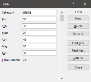
Show the table data entry form
If a table starts at cell A1, there is a simple data entry form that can be displayed.
Sub ShowDataEntryForm()

'Only works if Table starts at Cell A1
ActiveSheet.ShowDataForm

End Sub
The following screenshot shows the data form for the example table.
Check if a table exists
The following macro checks if a table already exists within a workbook. Change the tblName variable to adapt this to your requirements.
Sub CheckIfTableExists()

'Create variables to hold the worksheet and the table
Dim ws As Worksheet
Dim tbl As ListObject
Dim tblName As String
Dim tblExists As Boolean

tblName = "myTable"

'Loop through eac worksheet
For Each ws In ActiveWorkbook.Worksheets

    'Loop through each table in worksheet
    For Each tbl In ws.ListObjects

        If tbl.Name = tblName Then

            tblExists = True

        End If

    Next tbl

Next ws

If tblExists = True Then

    MsgBox "Table " & tblName & " exists."

Else

    MsgBox "Table " & tblName & " does not exists."

End If

End Sub
Find out if a table has been selected, if so which
The following macros find the name of the selected table.
Method 1
As you will see in the comments Jon Peltier had an easy approach to this, which has now become my preferred approach.
Sub SimulateActiveTable()

Dim ActiveTable As ListObject

On Error Resume Next
Set ActiveTable = ActiveCell.ListObject
On Error GoTo 0

'Confirm if a cell is in a Table
If ActiveTable Is Nothing Then
    MsgBox "Select table and try again"
Else
    MsgBox "The active cell is in a Table called: " & ActiveTable.Name
End If

End Sub
Method 2
This option, which was my original method, loops through each table on the worksheet and checks if they intersect with the active cell.
Sub SimulateActiveTable_Method2()

Dim ActiveTable As ListObject
Dim tbl As ListObject

'Loop through each table, check if table intersects with active cell
For Each tbl In ActiveSheet.ListObjects

    If Not Intersect(ActiveCell, tbl.Range) Is Nothing Then

        Set ActiveTable = tbl
        MsgBox "The active cell is in a Table called: " & ActiveTable.Name

    End If

Next tbl

'If no intersection then no tabl selected
If ActiveTable Is Nothing Then

    MsgBox "Select an Excel table and try again"

End If

End Sub
Conclusion
Wow! That was a lot of code examples.
There are over 30 VBA macros above, and even this does not cover everything, but hopefully covers 99% of your requirements. For your remaining requirements, you could try Microsoft’s VBA object reference library (https://docs.microsoft.com/en-us/office/vba/api/Excel.ListObject)

About the author
Hey, I’m Mark, and I run Excel Off The Grid.
My parents tell me that at the age of 7 I declared I was going to become a qualified accountant. I was either psychic or had no imagination, as that is exactly what happened. However, it wasn’t until I was 35 that my journey really began.
In 2015, I started a new job, for which I was regularly working after 10pm. As a result, I rarely saw my children during the week. So, I started searching for the secrets to automating Excel. I discovered that by building a small number of simple tools, I could combine them together in different ways to automate nearly all my regular tasks. This meant I could work less hours (and I got pay raises!). Today, I teach these techniques to other professionals in our training program so they too can spend less time at work (and more time with their children and doing the things they love).
Do you need help adapting this post to your needs?
I’m guessing the examples in this post don’t exactly match your situation. We all use Excel differently, so it’s impossible to write a post that will meet everybody’s needs. By taking the time to understand the techniques and principles in this post (and elsewhere on this site), you should be able to adapt it to your needs.
But, if you’re still struggling you should:
- Read other blogs, or watch YouTube videos on the same topic. You will benefit much more by discovering your own solutions.
- Ask the ‘Excel Ninja’ in your office. It’s amazing what things other people know.
- Ask a question in a forum like Mr Excel, or the Microsoft Answers Community. Remember, the people on these forums are generally giving their time for free. So take care to craft your question, make sure it’s clear and concise. List all the things you’ve tried, and provide screenshots, code segments and example workbooks.
- Use Excel Rescue, who are my consultancy partner. They help by providing solutions to smaller Excel problems.
What next?
Don’t go yet, there is plenty more to learn on Excel Off The Grid. Check out the latest posts:
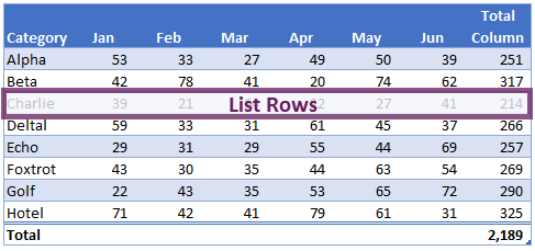
All About The Tables
For a data analyst, Excel Tables are a necessity! They are the most efficient way to organize your raw data and refer to data that contracts or expands on a regular basis. Likewise, Excel tables can be extremely useful in combination with VBA.
I personally use data tables as a way to store user settings without having to modify any VBA code. You can see examples of this in my Exporter Template where I use tables to store worksheet names and email addresses.
In this article, I wanted to bring all the common ways of referencing table data with VBA into one place. Hopefully, this will serve as a guide you can come back to again and again so you can easily and efficiently incorporate tables into your VBA macro coding. Enjoy!
Section Quick Links
-
Excel Tables Overview
-
Selecting Areas Of A Table With VBA
-
Inserting Rows and Columns Into The Table
-
Deleting Parts Of A Table
-
Deleting/Clearing The Data In A Table
-
Loop Through Each Table Column Or Row
-
Looking Up Values Within A Table
-
Apply A Sort Order To A Table Column
-
Reading Table Data Into An Array Variable
-
Resizing A Table
-
Change All Table Column’s Total Row Calculations
-
Getting To The ActiveTable
-
Additional Articles
Excel Tables Overview
What Is A Table?
A Table is simply a structured range where you can refer to different sections that are automatically mapped out (such as the Header Row or the column below the header «Amount»). Tables are an amazing feature that Microsoft added into Excel because they not only structure your data, but they also expand with your data as it grows. And if there is one thing you should know about creating a spreadsheet, it would be that making it as DYNAMIC as possible is always a good thing!
You can quickly create a Table by highlighting a range (with proper headings) and using the keyboard shortcut Ctrl + t. You can also navigate to the Insert tab and select the Table button within the Tables group.
The Parts of A Table
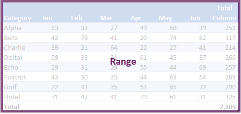
The below infographic will help you visualize the different parts of a Table object through the lens of the VBA coding language.
These parts of a ListObject Table include:
-
Range
-
HeaderRowRange
-
DataBodyRange
-
ListRows
-
ListColumns
-
TotalsRowRange

How Do I Find Existing Tables?
Tables can be a little tricky to find if you are not familiar working with them because they can blend in very well with the spreadsheet depending on the formatting that has been applied.
Let’s look at 4 different ways you can determine if you are working with cells in a Table Object.
1. The Table Design Tab Appears
If you click within a cell that is part of an Excel Table, you will immediately see the Table Design tab appear in the Ribbon. This is a contextual tab, which means it only appears when a specific object is selected on your spreadsheet (a similar tab appears when Pivot Tables or Shapes are selected on a spreadsheet).
This is a very quick tell-tail sign that the cell you are working on is part of a Table Object.
2. The Blue Corner Indicator
There is a small little indicator at the bottom right cell of a Table range to indicate there is a table. As you can see in the image below, this indicator can be very simple to find, but also can be easily missed due to its small size!

3. Use Excel’s Name Manager
Another great way to find a table (and its name) is to go into the Name Manager. You can get to the name manager by navigating to the Formulas tab and clicking the Name Manager button inside the Defined Names group.
By using the Filter menu in the right-hand corner of the Name Manager, you can narrow down your name list to just the Tables within the Workbook. The Name Manager will show you exactly where the tables are within the spreadsheet and also what the Table names are.
4. VBA Code To Check If Cell Is In A ListObject Table
There may be instances when you need to determine if a certain cell resides within a ListObject (Table). The below VBA code shows you how you can perform a test to see if the ActiveCell (selected cell) is part of any Excel Table on the spreadsheet.
Sub IsActiveCellInTable()
‘PURPOSE: Determine if the current selected cell is part of an Excel Table
‘SOURCE: www.TheSpreadsheetGuru.com
Dim TestForTable As String
‘Test To See If Cell Is Within A Table
On Error Resume Next
TestForTable = ActiveCell.ListObject.Name
On Error GoTo 0
‘Determine Results of Test
If TestForTable <> «» Then
‘ActiveCell is within a ListObject Table
MsgBox «Cell is part of the table named: » & TestForTable
Else
‘ActiveCell is NOT within a ListObject Table
MsgBox «Cell is not part of any table»
End If
End Sub
This is a great validation test if you are creating code that allows the user to manipulate an excel table. I’ve used this many times to create buttons that allow users to insert or delete specific rows within a table based on where they select on a password protected sheet.
Selecting Areas of a Table with VBA
| Select | VBA Coding |
|---|---|
| Entire Table | ActiveSheet.ListObjects(«Table1»).Range.Select |
| Table Header Row | ActiveSheet.ListObjects(«Table1»).HeaderRowRange.Select |
| Table Data | ActiveSheet.ListObjects(«Table1»).DataBodyRange.Select |
| Third Column | ActiveSheet.ListObjects(«Table1»).ListColumns(3).Range.Select |
| Third Column (Data Only) | ActiveSheet.ListObjects(«Table1»).ListColumns(3).DataBodyRange.Select |
| Select Row 4 of Table Data | ActiveSheet.ListObjects(«Table1»).ListRows(4).Range.Select |
| Select 3rd Heading | ActiveSheet.ListObjects(«Table1»).HeaderRowRange(3).Select |
| Select Data point in Row 3, Column 2 | ActiveSheet.ListObjects(«Table1»).DataBodyRange(3, 2).Select |
| Subtotals | ActiveSheet.ListObjects(«Table1»).TotalsRowRange.Select |
Inserting Rows and Columns into the Table
| Select | VBA Coding |
|---|---|
| Insert A New Column 4 | ActiveSheet.ListObjects(«Table1»).ListColumns.Add Position:=4 |
| Insert Column at End of Table | ActiveSheet.ListObjects(«Table1»).ListColumns.Add |
| Insert Row Above Row 5 | ActiveSheet.ListObjects(«Table1»).ListRows.Add (5) |
| Add Row To Bottom of Table | ActiveSheet.ListObjects(«Table1»).ListRows.Add AlwaysInsert:= True |
| Add Totals Row | ActiveSheet.ListObjects(«Table1»).ShowTotals = True |
Deleting Various Parts Of A Table
Sub RemovePartsOfTable()
Dim tbl As ListObject
Set tbl = ActiveSheet.ListObjects(«Table1»)
‘Remove 3rd Column
tbl.ListColumns(3).Delete
‘Remove 4th DataBody Row
tbl.ListRows(4).Delete
‘Remove 3rd through 5th DataBody Rows
tbl.Range.Rows(«3:5»).Delete
‘Remove Totals Row
tbl.TotalsRowRange.Delete
End Sub
Deleting/Clearing The Data In A Table
Delete all data rows from a table (except the first row)
Sub ResetTable()
Dim tbl As ListObject
Set tbl = ActiveSheet.ListObjects(«Table1»)
‘Delete all table rows except first row
With tbl.DataBodyRange
If .Rows.Count > 1 Then
.Offset(1, 0).Resize(.Rows.Count — 1, .Columns.Count).Rows.Delete
End If
End With
‘Clear out data from first table row
tbl.DataBodyRange.Rows(1).ClearContents
End Sub
If you have formulas in your table, you may want to keep those intact. The following modification will just remove constant values from the remaining first row in the Table Object.
Sub ResetTable()
Dim tbl As ListObject
Set tbl = ActiveSheet.ListObjects(«Table1»)
‘Delete all table rows except first row
With tbl.DataBodyRange
If .Rows.Count > 1 Then
.Offset(1, 0).Resize(.Rows.Count — 1, .Columns.Count).Rows.Delete
End If
End With
‘Clear out data from first table row (retaining formulas)
tbl.DataBodyRange.Rows(1).SpecialCells(xlCellTypeConstants).ClearContents
End Sub
Loop Through Each Table Column Or Row
Sub LoopingThroughTable()
Dim tbl As ListObject
Dim x As Long
Set tbl = ActiveSheet.ListObjects(«Table1»)
‘Loop Through Each Column in Table
For x = 1 To tbl.ListColumns.Count
tbl.ListColumns(x).Range.ColumnWidth = 8
Next x
‘Loop Through Every Row in Table
For x = 1 To tbl.Range.Rows.Count
tbl.Range.Rows(x).RowHeight = 20
Next x
‘Loop Through Each DataBody Row in Table
For x = 1 To tbl.ListRows.Count
tbl.ListRows(x).Range.RowHeight = 15
Next x
End Sub
Apply Sort To Column In A Table
You may find yourself needing to sort your Table data in either Ascending or Descending order. The following VBA code will show you how to sort a column in your ListObject Table in either order.
Sub SortTableColumn()
‘PUPOSE: Sort Table in Ascending/Descending Order
‘SOURCE: www.TheSpreadsheetGuru.com
Dim tbl As ListObject
Dim SortOrder As Integer
‘Choose Sort Order
SortOrder = xlAscending ‘(or xlDescending)
‘Store Desired Excel Table to a variable
Set tbl = ActiveSheet.ListObjects(«Table1»)
‘Clear Any Prior Sorting
tbl.Sort.SortFields.Clear
‘Apply A Sort on Column 1 of Table
tbl.Sort.SortFields.Add2 _
Key:=tbl.ListColumns(1).Range, _
SortOn:=xlSortOnValues, _
Order:=SortOrder, _
DataOption:=xlSortNormal
‘Sort Options (if you want to change from default)
tbl.Sort.Header = xlYes
tbl.Sort.MatchCase = False
tbl.Sort.Orientation = xlTopToBottom
tbl.Sort.SortMethod = xlPinYin
‘Apply the Sort to the Table
tbl.Sort.Apply
End Sub
While the above VBA code has all the potential options written out for you to tweak, most of the time you will not need to stray away from the default sorting options.
Below is the same code, but with all the options you likely don’t need to change from their default setting value removed.
Sub SortTableColumn_Simple()
‘PUPOSE: Sort Table in Ascending/Descending Order
‘SOURCE: www.TheSpreadsheetGuru.com
Dim tbl As ListObject
Dim SortOrder As Integer
‘Choose Sort Order
SortOrder = xlDescending ‘(or xlAscending)
‘Store Desired Excel Table to a variable
Set tbl = ActiveSheet.ListObjects(«Table1»)
‘Clear Any Prior Sorting
tbl.Sort.SortFields.Clear
‘Apply A Sort on Column 1 of Table
tbl.Sort.SortFields.Add2 _
Key:=tbl.ListColumns(1).Range, _
Order:=SortOrder
‘Apply the Sort to the Table
tbl.Sort.Apply
End Sub
Looking Up Values Within A Table
If you are storing values inside a Table, there may be scenarios where you wish to look up or find a value. There are many different lookup scenarios one might have, but for simplicity, I will provide a generic example. The following code looks to find an ID string within a specific table’s first column and returns that ID’s table row number. Hopefully, you can use the logic within this example and apply it to your specific needs.
Sub LookupTableValue()
Dim tbl As ListObject
Dim FoundCell As Range
Dim LookupValue As String
‘Lookup Value
LookupValue = «ID-123»
‘Store Table Object to a variable
Set tbl = ActiveSheet.ListObjects(«Table1»)
‘Attempt to find value in Table’s first Column
On Error Resume Next
Set FoundCell = tbl.DataBodyRange.Columns(1).Find(LookupValue, LookAt:=xlWhole)
On Error GoTo 0
‘Return Table Row number if value is found
If Not FoundCell Is Nothing Then
MsgBox «Found in table row: » & _
tbl.ListRows(FoundCell.Row — tbl.HeaderRowRange.Row).Index
Else
MsgBox «Value not found»
End If
End Sub
Store Table Data In An Array Variable
Pulling in data from tables is a great tactic to incorporate in your VBA coding. Tables are ideal because they:
-
Are always structured the same
-
Can be moved anywhere on the spreadsheet without affecting your code
-
Automatically adjust their range size
One example of using Tables as a data source in a macro is shown in one of my Code Vault snippets which allows you to filter your data based on the words in a specified table. There are tons of different ways you can use tables to store settings and preferences dynamically for your macros. The below code shows you how to load in data from a single column and a multi-column table.
Single Column Table
Sub SingleColumnTable_To_Array()
Dim myTable As ListObject
Dim myArray As Variant
Dim TempArray As Variant
Dim x As Long
‘Set path for Table variable
Set myTable = ActiveSheet.ListObjects(«Table1»)
‘Create Array List from Table
TempArray = myTable.DataBodyRange
‘Convert from vertical to horizontal array list
myArray = Application.Transpose(TempArray)
‘Loop through each item in the Table Array (displayed in Immediate Window [ctrl + g])
For x = LBound(myArray) To UBound(myArray)
Debug.Print myArray(x)
Next x
End Sub
Multiple Column Table
Sub MultiColumnTable_To_Array()
Dim myTable As ListObject
Dim myArray As Variant
Dim x As Long
‘Set path for Table variable
Set myTable = ActiveSheet.ListObjects(«Table1»)
‘Create Array List from Table
myArray = myTable.DataBodyRange
‘Loop through each item in Third Column of Table (displayed in Immediate Window [ctrl + g])
For x = LBound(myArray) To UBound(myArray)
Debug.Print myArray(x, 3)
Next x
End Sub
Resizing A Table
If needed, you can resize a table’s dimensions by declaring a new range area for the Excel table to shrink or expand. Below are a couple of examples showing how you can perform this sort of size adjustment.
(A special thanks to Peter Bartholomew for requesting this on LinkedIn)
Sub ResizeTable()
Dim rng As Range
Dim tbl As ListObject
‘Resize Table to 7 rows and 5 columns
Set rng = Range(«Table1[#All]»).Resize(7, 5)
ActiveSheet.ListObjects(«Table1»).Resize rng
‘Expand Table size by 10 rows
Set tbl = ActiveSheet.ListObjects(«Table1»)
Set rng = Range(tbl.Name & «[#All]»).Resize(tbl.Range.Rows.Count + 10, tbl.Range.Columns.Count)
tbl.Resize rng
End Sub
Change All Table Total Row Calculations
Sub ChangeAllColumnTotals()
Dim tbl As ListObject
Dim CalcType As Integer
Dim x As Long
Set tbl = ActiveSheet.ListObjects(«Table1»)
‘What calculation should the Totals Row Have?
CalcType = 1 ‘or: xlTotalsCalculationSum
‘Loop Through All Table Columns
For x = 1 To tbl.ListColumns.Count
tbl.ListColumns(x).TotalsCalculation = CalcType
Next x
‘___________________________________________
‘Members of xlTotalsCalculation
‘Enum Calculation
‘ 0 None
‘ 1 Sum
‘ 2 Average
‘ 3 Count
‘ 4 Count Numbers
‘ 5 Min
‘ 6 Max
‘ 7 Std Deviation
‘ 8 Var
‘ 9 Custom
‘___________________________________________
End Sub
Getting the ActiveTable
There may be instances where you want to make a personal macro that formats your selected table in a certain way or adds certain calculation columns. Since the Excel developers didn’t create an ActiveTable command in their VBA language, you have no straightforward way of manipulating a user-selected table. But with a little creativity, you can make your own ActiveTable ListObject variable and do whatever you want with the selected table!
Sub DetermineActiveTable()
Dim SelectedCell As Range
Dim TableName As String
Dim ActiveTable As ListObject
Set SelectedCell = ActiveCell
‘Determine if ActiveCell is inside a Table
On Error GoTo NoTableSelected
TableName = SelectedCell.ListObject.Name
Set ActiveTable = ActiveSheet.ListObjects(TableName)
On Error GoTo 0
‘Do something with your table variable (ie Add a row to the bottom of the ActiveTable)
ActiveTable.ListRows.Add AlwaysInsert:=True
Exit Sub
‘Error Handling
NoTableSelected:
MsgBox «There is no Table currently selected!», vbCritical
End Sub
Visual Learner? Download My Example Workbook
Screenshot from one of the tabs in the downloadable file
After many requests, I put together a fun little interactive workbook that will show you how a bunch of the code described in this article actually works on a spreadsheet. It also serves as a good reference that you can save to your computer so you don’t have to keep googling about Excel Tables whenever something slips your mind.
Download Example Excel File
If you would like to get a copy of the Excel file I used throughout this article, feel free to directly download the spreadsheet by clicking the download button below.
Anything Else About Tables I Missed?
Did you come to this page trying to find out how to do something with VBA and Excel tables and it wasn’t covered? If that is the case, let me know what you were looking for in the comment section below. If it makes sense to add it to this guide and will definitely add it to the content. I look forward to reading your thoughts and/or recommendations!

About The Author
Hey there! I’m Chris and I run TheSpreadsheetGuru website in my spare time. By day, I’m actually a finance professional who relies on Microsoft Excel quite heavily in the corporate world. I love taking the things I learn in the “real world” and sharing them with everyone here on this site so that you too can become a spreadsheet guru at your company.
Through my years in the corporate world, I’ve been able to pick up on opportunities to make working with Excel better and have built a variety of Excel add-ins, from inserting tickmark symbols to automating copy/pasting from Excel to PowerPoint. If you’d like to keep up to date with the latest Excel news and directly get emailed the most meaningful Excel tips I’ve learned over the years, you can sign up for my free newsletters. I hope I was able to provide you some value today and hope to see you back here soon! — Chris
The Data table is similar to the Scenario Manager and Goal Seek and does the same prediction function.
A data table is a range of cells in which you can change values in some of the cells and come up with different answers to a problem
There are two types of Data tables; One Variable data table and Two variable data table.
For illustration purpose, we will consider the One-variable data table.
One-variable data table is used while analyzing how different values of one variable in one or more formulas will change the results of those formulas.
The following example illustrates the use of Data table.
Let us build a data table that shows the monthly payments for loan terms ranging from 1 to 6 years.
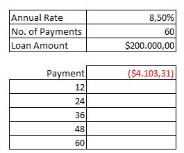
The Cells C10 to C12 contains the Loan details.
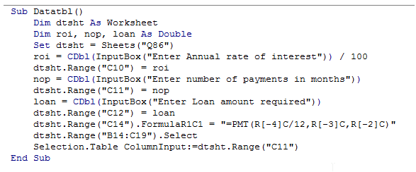
The following code shows how to create a datatable in the range B14:C19
- Sub Datatbl()
- Dim dtsht As Worksheet
- Dim roi, nop, loan As Double
- Set dtsht = Sheets(«Q86»)
- roi = CDbl(InputBox(«Enter Annual rate of interest»)) / 100
- dtsht.Range(«C10») = roi
- nop = CDbl(InputBox(«Enter number of payments in months»))
- dtsht.Range(«C11») = nop
- loan = CDbl(InputBox(«Enter Loan amount required»))
- dtsht.Range(«C12») = loan
- dtsht.Range(«C14»).FormulaR1C1 = «=PMT(R[-4]C/12,R[-3]C,R[-2]C)»
- dtsht.Range(«B14:C19»).Select
- Selection.Table ColumnInput:=dtsht.Range(«C11»)
- End Sub
When executed, the program will demand the user to input Rate of Interest, Payment period and Loan amount.
Once entered, the program will create a datatable in the range B14:C19, corresponding to the values in B14:B19.
The screenshot of the editor is as shown below.
You can find similar Excel Questions and Answer hereunder
1) How can I extract file name from a full path including folder path and file name?
2) How to import data from Microsoft Access into Excel using VBA
3) Vba code to password protect workbook in Excel
4) Vba list all files in a folder in Excel
5) Here a explanation about the global seek function in VBA. Goal Seek is another tool under What If analysis that does a unique function as Scenario Manager.
6) How can I list all files in a folder using VBA?
7) How can I convert Column numbers into Column names for use in range definition?
 How can I add Trendline to a chart using VBA?
9) How can I hide all comments in my WorkSheet using VBA?
10) How to import xml data into Excel using VBA
Tables in Excel VBA – Explained with Examples!
Managing the data with Tables is very easy in Excel. We can do lot more things if your data is in the form of tables. In this section we will show some of the Tables operations using Excel VBA.
- Create Tables in Excel VBA
- Sorting Tables in Excel VBA
- Filtering Tables in Excel VBA
- Clear Toggle Table Filters in Excel VBA
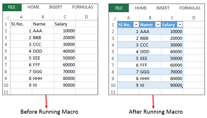
Create Tables in Excel VBA:
Sometimes you may want to create Tables in Excel VBA. Please find the following code to Create Tables in Excel VBA.
- Solution
- Code
- Output
- Reset a Table back to Normal Range
- Example File
Create Tables in Excel VBA – Solution(s):
You can use ListObjects.Add method of sheet to create tables in excel VBA. We can create table in the following way. The following code creates a table “myTable1” and referring to sheet1 of a range(“$A$1:$D$10”) .
Code:
'Naming a range
Sub sbCreatTable()

    'Create Table in Excel VBA
    Sheet1.ListObjects.Add(xlSrcRange, Range("A1:D10"), , xlYes).Name = "myTable1"

End Sub
Output:
Instructions:
- Open an excel workbook
- Press Alt+F11 to open VBA Editor
- Double click on ThisWorkbook from Project Explorer
- Copy the above code and Paste in the code window
- Press F5
- GoTo Sheet1 and Select Range A1 to D10
- You should see the above output in Sheet1
Reset a Table back to Normal Range
If you want to Reset the table back to original range, you can use Unlist property of table object. Following code will show you how to remove table formats and reset to normal range.
Sub sbReset_Table_BackTo_Range()

    'Reset Table Back to Original Range
    On Error Resume Next  'If there are no Table ignore the below Statement
    Sheet1.ListObjects("myTable1").Unlist

End Sub
Example File
Download the example file and Explore it.
Analysistabs – Create Tables in Excel VBA
Sorting Tables in Excel VBA:
Examples for Sorting Table in Excel VBA with using sort method of ListObjects. You can learn how to sort table with examples.
- Solution
- Code
- Output
Sorting Table in Excel VBA – Solution(s):
You can use sort method of ListObjects for sorting table in Excel VBA. We can do sort data in the following way.
Code:
Sub sbSortTable()

     'Naming a range
     Sheet1.Sheets("Sheet1").ListObjects("myTable1").Sort.SortFields.Clear
     Sheet1.Sheets("Sheet1").ListObjects("myTable1").Sort.SortFields.Add Key:=Range("myTable1[[#All],[EmpName]]"), SortOn:=sortonvalues, Order:=xlAscending, DataOption:=xlSortNormal
     Range("myTable1[#All]").Select
     With Sheet1.Worksheets("Sheet1").ListObjects("myTable1").Sort
        .Header = xlYes
        .MatchCase = False
        .Orientation = xlTopToBottom
        .SortMethod = xlPinYin
        .Apply
    End With

End Sub
Output:
Instructions:
- Open an excel workbook
- Press Alt+F11 to open VBA Editor
- Double click on ThisWorkbook from Project Explorer
- Copy the above code and Paste in the code window
- Press F5
- GoTo Sheet1 and Select Range A1 to D10
- You should see the above output in Sheet1
Filtering Tables in Excel VBA
Sometimes you may want to Filter Tables in Excel VBA. Please find the following code for Filtering Tables in Excel VBA.
- Solution
- Code
- Output
- Example File
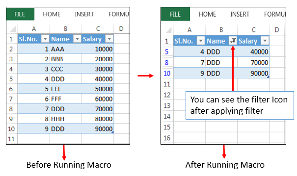
Filtering Tables in Excel VBA – Solution(s):
You can use ListObjects(“TableName”).Range.AutoFilter method for Filtering tables in excel VBA. We can filter table in the following way. The following code filters a table “myTable1” and referring to sheet1 of a range(“$A$1:$D$10”).In this Case I am applying filter for second column and looking for description “DDD” in a table.
Code:
'Filtering a table
Sub sbFilterTable()

     ActiveWorkbook.Sheets("Sheet1").ListObjects("myTable1").Range.AutoFilter field:=2, Criteria1:="DDD" 'matched with 4 in column c2 records will be shown

End Sub
Output:
Instructions:
- Open an excel workbook
- Press Alt+F11 to open VBA Editor
- Double click on ThisWorkbook from Project Explorer
- Copy the above code and Paste in the code window
- Press F5 to execute Macro
- GoTo Sheet1 and Select Range A1 to D10
- You should see the above output in Sheet1
Example File
Download the example file and Explore it.
Analysistabs – Filtering Tables in Excel VBA
Clear or Toggle Table Filters in Excel VBA:
Examples for Clear Toggle Table Filters in Excel VBA with using FilterMode Property and AutoFilter method. You can learn how to Clear Toggle Table Filters in Excel VBA with following example.
- Solution
- Code
- Output
- Example File
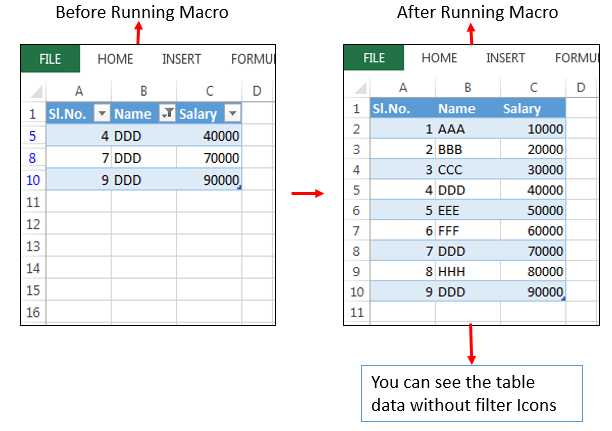
Clear Toggle Table Filters in Excel VBA – Solution(s):
You can Clear Toggle Table Filters in Excel VBA with using FilterMode Property and AutoFilter method in Excel VBA. We can do Clear table filter in the following way.
Code:
'Clear Table Filter
Sub sbClearFilter()

    'Check Filter is Exists or Not
    If ActiveWorkbook.Sheets("Sheet1").FilterMode = True Then

        ActiveWorkbook.Sheets("Sheet1").ListObjects("myTable1").Range.AutoFilter

    End If

End Sub
Output:
Instructions:
- Open an excel workbook
- Press Alt+F11 to open VBA Editor
- Double click on ThisWorkbook from Project Explorer
- Copy the above code and Paste in the code window
- Press F5 to execute Macro
- GoTo Sheet1 and check the Table Data from A1 to D10
- You should see the above output in Sheet1
Example File
Download the example file and Explore it.
Analysistabs – Clear Tables in Excel VBA
A Powerful & Multi-purpose Templates for project management. Now seamlessly manage your projects, tasks, meetings, presentations, teams, customers, stakeholders and time. This page describes all the amazing new features and options that come with our premium templates.
Save Up to 85% LIMITED TIME OFFER

All-in-One Pack
120+ Project Management Templates
Essential Pack
50+ Project Management Templates
Excel Pack
50+ Excel PM Templates
PowerPoint Pack
50+ Excel PM Templates
MS Word Pack
25+ Word PM Templates
Ultimate Project Management Template
Ultimate Resource Management Template
Project Portfolio Management Templates
Related Posts
-
- Create Tables in Excel VBA:
- Create Tables in Excel VBA – Solution(s):
- Sorting Tables in Excel VBA:
- Sorting Table in Excel VBA – Solution(s):
- Filtering Tables in Excel VBA
- Filtering Tables in Excel VBA – Solution(s):
- Clear or Toggle Table Filters in Excel VBA:
- Clear Toggle Table Filters in Excel VBA – Solution(s):
VBA Reference
Effortlessly
Manage Your Projects
120+ Project Management Templates
Seamlessly manage your projects with our powerful & multi-purpose templates for project management.
120+ PM Templates Includes:
13 Comments
-
Bruce
January 13, 2014 at 2:20 AM — ReplyExcellent! Now the couple pieces missing:
1) Copying the filtered results to a new sheet Sheet02 (and whether or not the copied area is a range, table or neither at that time)
2)Applying the same process to a new range of data and adding that filtered section to the previously established data on the new sheet Sheet02
3) Sorting the new sheet data every time data is added and removing duplicates based upon one field being used as a key.I am sure I will run into all this, but you folks were off to such a great start of the information being clear and collected in one place, I wanted to place the suggestion, provided you ever have the time!
-
PNRao
January 13, 2014 at 9:14 PM — ReplyHi Bruce,
Thanks for your suggestion, I will add these in couple of weeks.
Thanks-PNRao!
-
Nurit
May 27, 2014 at 10:11 PM — ReplyHow do you create a table when the range is dynamic. I want to automate the process of refreshing and opening pivot tables. I need to:
1) import data from a software package (this will be done manually)
2) open the file created in #1 and create and name table. The range of data is unknown.
3) open the pivot table which will refresh automatically using the named table created in #2.I got this far – how do I change the defined range to a dynamic range and do I need the last line?
Sub opengetfile()
Dim strFileName As String
Dim rgData As Range
strFileName = Application.GetOpenFilename
If strFileName = “False” Then Exit Sub
MsgBox strFileName
Workbooks.Open (strFileName)ActiveSheet.ListObjects.Add(xlSrcRange, Range(“$A$1:$AX$224”), , xlYes).Name = “Loans”
Range(“Loans[#All]”).SelectEnd Sub
-
PNRao
May 28, 2014 at 11:45 PM — Reply -
Gejza Horvath
June 16, 2014 at 1:42 AM — ReplyIf all the data on this sheet will be inside a listobject, you can use ActiveSheet.UsedRange property. Instead the Range() object.
-
JonasTiger
December 29, 2014 at 3:44 AM — ReplyHi
Filtering Tables in Excel VBA…
I need to filter my table everytime data changes.
In your example, you filter “DDD”.
In mine, I want filter all options except zero/blank cells of a range, i.e., its like excluding “DDD” and leave remaining data.
please help me changing code for that.
Thank you -
Amy
January 30, 2015 at 5:27 AM — ReplyThis has been very helpful! I needed to create a macro to turn a dynamic range into a table, sort by a specific column, & filter the table based on that same column name. This page had all the information I needed.
I look forward to checking out the other areas of your site.Thanks for sharing.
-
yonsebastian
June 1, 2015 at 5:52 AM — Replyworking for year with VBA now 2013 comes with tables which is awesome!
-
PNRao
June 1, 2015 at 12:20 PM — ReplyYes, Tables or ListObjects in Excel are very handy to deal with the data. We can perform many operations and its fast.
Thanks-PNRao!
-
Agni
June 10, 2016 at 12:31 PM — ReplyHi,
How to create a table without default auto filter and header. -
prema
April 2, 2018 at 11:49 AM — ReplyIf ActiveWorkbook.Sheets(“Sheet1”).FilterMode = True Then
is not working for a listobject
-
a
February 17, 2020 at 9:28 AM — Reply[code]
Sub Next ()
If G3=1 Then
Next i
Me.ListBox1.Column = Tbl
End If
End Sub -
a
February 17, 2020 at 9:29 AM — Reply[code]
Sub Next ()
If G3=1 Then
Next i
Me.ListBox1.Column = Tbl
End If
End Sub
[/code]
Effectively Manage Your
Projects and Resources
ANALYSISTABS.COM provides free and premium project management tools, templates and dashboards for effectively managing the projects and analyzing the data.
We’re a crew of professionals expertise in Excel VBA, Business Analysis, Project Management. We’re Sharing our map to Project success with innovative tools, templates, tutorials and tips.
Project Management
Excel VBA
Download Free Excel 2007, 2010, 2013 Add-in for Creating Innovative Dashboards, Tools for Data Mining, Analysis, Visualization. Learn VBA for MS Excel, Word, PowerPoint, Access, Outlook to develop applications for retail, insurance, banking, finance, telecom, healthcare domains.
Page load link
Go to Top