
A data table is a range of cells in which you can change values in some of the cells and come up with different answers to a problem. A good example of a data table employs the PMT function with different loan amounts and interest rates to calculate the affordable amount on a home mortgage loan. Experimenting with different values to observe the corresponding variation in results is a common task in data analysis.
In Microsoft Excel, data tables are part of a suite of commands known as What-If analysis tools. When you construct and analyze data tables, you are doing what-if analysis.
What-if analysis is the process of changing the values in cells to see how those changes will affect the outcome of formulas on the worksheet. For example, you can use a data table to vary the interest rate and term length for a loan—to evaluate potential monthly payment amounts.
Types of what-if analysis
There are three types of what-if analysis tools in Excel: scenarios, data tables, and goal-seek. Scenarios and data tables use sets of input values to calculates possible results. Goal-seek is distinctly different, it uses a single result and calculates possible input values that would produce that result.
Like scenarios, data tables help you explore a set of possible outcomes. Unlike scenarios, data tables show you all the outcomes in one table on one worksheet. Using data tables makes it easy to examine a range of possibilities at a glance. Because you focus on only one or two variables, results are easy to read and share in tabular form.
A data table cannot accommodate more than two variables. If you want to analyze more than two variables, you should instead use scenarios. Although it is limited to only one or two variables (one for the row input cell and one for the column input cell), a data table can include as many different variable values as you want. A scenario can have a maximum of 32 different values, but you can create as many scenarios as you want.
Learn more in the article, Introduction to What-If Analysis.
Create either one-variable or two-variable data tables, depending on the number of variables and formulas that you need to test.
One-variable data tables
Use a one-variable data table if you want to see how different values of one variable in one or more formulas will change the results of those formulas. For example, you can use a one-variable data table to see how different interest rates affect a monthly mortgage payment by using the PMT function. You enter the variable values in one column or row, and the outcomes are displayed in an adjacent column or row.
In the following illustration, cell D2 contains the payment formula, =PMT(B3/12,B4,-B5), which refers to the input cell B3.
Two-variable data tables
Use a two-variable data table to see how different values of two variables in one formula will change the results of that formula. For example, you can use a two-variable data table to see how different combinations of interest rates and loan terms will affect a monthly mortgage payment.
In the following illustration, cell C2 contains the payment formula, =PMT(B3/12,B4,-B5), which uses two input cells, B3 and B4.
Data table calculations
Whenever a worksheet recalculates, any data tables will also recalculate—even if there has been no change to the data. To speed up calculation of a worksheet that contains a data table, you can change the Calculation options to automatically recalculate the worksheet but not the data tables. To learn more, see the section Speed up calculation in a worksheet that contains data tables.
A one-variable data table contain its input values either in a single column (column-oriented), or across a row (row-oriented). Any formula in a one-variable data table must refer to only one input cell.
Follow these steps:
-
Type the list of values that you want to substitute in the input cell—either down one column or across one row. Leave a few empty rows and columns on either side of the values.
-
Do one of the following:
-
If the data table is column-oriented (your variable values are in a column), type the formula in the cell one row above and one cell to the right of the column of values. This one-variable data table is column-oriented, and the formula is contained in cell D2.

If you want to examine the effects of various values on other formulas, enter the additional formulas in cells to the right of the first formula.
-
If the data table is row-oriented (your variable values are in a row), type the formula in the cell one column to the left of the first value and one cell below the row of values.
If you want to examine the effects of various values on other formulas, enter the additional formulas in cells below the first formula.
-
-
Select the range of cells that contains the formulas and values that you want to substitute. In the figure above, this range is C2:D5.
-
On the Data tab, click What-If Analysis > Data Table (in the Data Tools group or Forecast group of Excel 2016).
-
Do one of the following:
-
If the data table is column-oriented, enter the cell reference for the input cell in the Column input cell field. In the figure above, the input cell is B3.
-
If the data table is row-oriented, enter the cell reference for the input cell in the Row input cell field.
Note: After you create your data table, you might want to change the format of the result cells. In the figure, the result cells are formatted as currency.
-
Formulas that are used in a one-variable data table must refer to the same input cell.
Follow these steps
-
Do either of these:
-
If the data table is column-oriented, enter the new formula in a blank cell to the right of an existing formula in the top row of the data table.
-
If the data table is row-oriented, enter the new formula in a empty cell below an existing formula in the first column of the data table.
-
-
Select the range of cells that contains the data table and the new formula.
-
On the Data tab, click What-If Analysis > Data Table (in the Data Tools group or Forecast group of Excel 2016).
-
Do either of the following:
-
If the data table is column-oriented, enter the cell reference for the input cell in the Column input cell box.
-
If the data table is row-oriented, enter the cell reference for the input cell in the Row input cell box.
-
A two-variable data table uses a formula that contains two lists of input values. The formula must refer to two different input cells.
Follow these steps:
-
In a cell on the worksheet, enter the formula that refers to the two input cells.
In the following example—in which the formula starting values are entered in cells B3, B4, and B5, you type the formula =PMT(B3/12,B4,-B5) in cell C2.
-
Type one list of input values in the same column, below the formula.
In this case, type the different interest rates in cells C3, C4, and C5.
-
Enter the second list in the same row as the formula—to its right.
Type the loan terms (in months) in cells D2 and E2.
-
Select the range of cells that contains the formula (C2), both the row and column of values (C3:C5 and D2:E2), and the cells in which you want the calculated values (D3:E5).
In this case, select the range C2:E5.
-
On the Data tab, in the Data Tools group or Forecast group (in Excel 2016), click What-If Analysis > Data Table (in the Data Tools group or Forecast group of Excel 2016).
-
In the Row input cell field, enter the reference to the input cell for the input values in the row.
Type cell B4 in the Row input cell box. -
In the Column input cell field, enter the reference to the input cell for the input values in the column.
Type B3 in the Column input cell box. -
Click OK.
Example of a two-variable data table
A two-variable data table can show how different combinations of interest rates and loan terms will affect a monthly mortgage payment. In the figure here, cell C2 contains the payment formula, =PMT(B3/12,B4,-B5), which uses two input cells, B3 and B4.
When you set this calculation option, no data-table calculations occur when a recalculation is done on the entire workbook. To manually recalculate your data table, select its formulas and then press F9.
Follow these steps to improve calculation performance:
-
Click File > Options > Formulas.
-
In the Calculation options section, under Calculate, click Automatic except for data tables.
Tip: Optionally, on the Formulas tab, click the arrow on Calculation Options, then click Automatic Except Data Tables (in the Calculation group).
You can use a few other Excel tools to perform what-if analysis if you have specific goals or larger sets of variable data.
Goal Seek
If you know the result to expect from a formula, but don’t know precisely what input value the formula needs to get that result, use the Goal-Seek feature. See the article Use Goal Seek to find the result you want by adjusting an input value.
Excel Solver
You can use the Excel Solver add-in to find the optimal value for a set of input variables. Solver works with a group of cells (called decision variables, or simply variable cells) that are used in computing the formulas in the objective and constraint cells. Solver adjusts the values in the decision variable cells to satisfy the limits on constraint cells and produce the result you want for the objective cell. Learn more in this article: Define and solve a problem by using Solver.
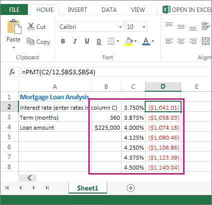
By plugging different numbers into a cell, you can quickly come up with different answers to a problem. A great example is using the PMT function with different interest rates and loan periods (in months) to figure out how much of a loan you can afford for a home or a car. You enter your numbers into a range of cells called a data table.
Here, the data table is the range of cells B2:D8. You can change the value in B4, the loan amount, and the monthly payments in column D automatically update. Using a 3.75% interest rate, D2 returns a monthly payment of $1,042.01 using this formula: =PMT(C2/12,$B$3,$B$4).
You can use one or two variables, depending on the number of variables and formulas you want to test.
Use a one-variable test to see how different values of one variable in a formula will change the results. For example, you can change the interest rate for a monthly mortgage payment by using the PMT function. You enter the variable values (the interest rates) in one column or row, and the outcomes are displayed in a nearby column or row.
In this live workbook, cell D2 contains the payment formula =PMT(C2/12,$B$3,$B$4). Cell B3 is the variable cell, where you can plug in a different term length (number of monthly payment periods). In cell D2, the PMT function plugs in the interest rate 3.75%/12, 360 months, and a $225,000 loan, and calculates a $1,042.01 monthly payment.
Use a two-variable test to see how different values of two variables in a formula will change the results. For example, you can test different combinations of interest rates and number of monthly payment periods to calculate a mortgage payment.
In this live workbook, cell C3 contains the payment formula, =PMT($B$3/12,$B$2,B4), which uses two variable cells, B2 and B3. In cell C2, the PMT function plugs in the interest rate 3.875%/12, 360 months, and a $225,000 loan, and calculates a $1,058.03 monthly payment.
Need more help?
You can always ask an expert in the Excel Tech Community or get support in the Answers community.
Таблица данных в Excel представляет собой диапазон, который оценивает изменение одной или двух переменных в формуле. Другими словами, это Анализ «что если», о котором мы говорили в одной из прошлых статей (если Вы ее не читали — очень рекомендую ознакомиться по этой ссылке), в удобном виде. Вы можете создать таблицу данных с одной или двумя переменными.

Предположим, что у Вас есть книжный магазин и в нем есть 100 книг на продажу. Вы можете продать определенный % книг по высокой цене — $50 и определенный % книг по более низкой цене — $20. Если Вы продаете 60% книг по высокой цене, в ячейке D10 вычисляется общая выручка по форуме 60 * $50 + 40 * $20 = $3800.
Скачать рассматриваемый пример Вы можете по этой ссылке: Пример анализа «что если» в Excel.
Таблица данных с одной переменной.
Что бы создать таблицу данных с одной переменной, выполните следующие действия:
1. Выберите ячейку B12 и введите =D10 (ссылка на общую выручку).
2. Введите различные проценты в столбце А.
3. Выберите диапазон A12:B17.
Мы будет рассчитывать общую выручку, если Вы продаете 60% книг по высокой цене, 70% книг по высокой цене и т.д.

4. На вкладке Данные, кликните на Анализ «что если» и выберите Таблица данных из списка.

5. Кликните в поле «Подставлять значения по строкам в: «и выберите ячейку C4.

Мы выбрали ячейку С4 потому что проценты относятся к этой ячейке (% книг, проданных по высокой цене). Вместе с формулой в ячейке B12, Excel теперь знает, что он должен заменять значение в ячейке С4 с 60% для расчета общей выручки, на 70% и так далее.
Примечание: Так как мы создает таблицу данных с одной переменной, то вторую ячейку ввода («Подставлять значения по столбцам в: «) мы оставляем пустой.
6. Нажмите ОК.
Результат.

Вывод: Если Вы продадите 60% книг по высокой цене, то Вы получите общую выручку в размере $3 800, если Вы продадите 70% по высокой цене, то получите $4 100 и так далее.
Примечание: Строка формул показывает, что ячейки содержат формулу массива. Таким образом, Вы не можете удалить один результат. Что бы удалить результаты, выделите диапазон B13:B17 и нажмите Delete.
Таблица данных с двумя переменными.
Что бы создать таблицу с двумя переменными, выполните следующие шаги.
1. Выберите ячейку A12 и введите =D10 (ссылка на общую выручку).
2. Внесите различные варианты высокой цены в строку 12.
3. Введите различные проценты в столбце А.
4. Выберите диапазон A12:D17.
Мы будем рассчитывать выручку от реализации книг в различных комбинациях высокой цены и % продаж книг по высокой цене.

5. На вкладке Данные, кликните на Анализ «что если» и выберите Таблица данных из списка.

6. Кликните в поле «Подставлять значения по столбцам в: » и выберите ячейку D7.
7. Кликните в поле «Подставлять значения по строкам в: » и выберите ячейку C4.
Мы выбрали ячейку D7, потому что высокая цена на книги задается именно в этой ячейке. Мы выбрали ячейку C4, потому что процент продаж по высокой цене задается именно в этой ячейке. Вместе с формулой в ячейке A12, Excel теперь знает, что он должен заменять значение ячейки D7 начиная с $50 и в ячейке С4 начиная с 60% для расчета общей выручки, до $70 и 100% соответсвенно.

8. Нажмите ОК.
Результат.

Вывод: Если Вы продадите 60% книг по высокой цене в размере $50, то Вы получите общую выручку $3 800, если Вы продадите 80% по высокой цене в размере $60, то получите $5 200 и так далее.
Примечание: строка формул показывает, что ячейки содержат формулу массива. Таким образом, вы не можете удалить один результат. Что бы удалить результаты, выделите диапазон B13:D17 и нажмите Delete.
Спасибо за внимание. Теперь Вы сможете более эффективно применять один из видов анализа «что если» , а именно формирование таблиц данных с одной или двумя переменными.
Остались вопросы — задавайте их в комментариях ниже, также не забывайте подписываться на нас в социальных сетях.
Содержание
- Таблица данных в Excel (типы, примеры) — Как создать таблицу данных в Excel
- Таблица данных в Excel
- Как создать таблицу данных в Excel?
- Таблица данных в Excel Пример № 1 — Таблица данных с одной переменной
- Таблица данных в Excel Пример № 2 — Таблица двух переменных данных
- Что нужно помнить о таблице данных в Excel
- Рекомендуемые статьи
- Таблица данных с одной переменной.
- Таблица данных с двумя переменными.
- Calculate multiple results by using a data table
- Need more help?
Таблица данных в Excel (типы, примеры) — Как создать таблицу данных в Excel

Таблица данных в Excel (Содержание)
- Таблица данных в Excel
- Как создать таблицу данных в Excel?
Таблица данных в Excel
Таблицы данных используются для анализа изменений, которые видны в вашем конечном результате, когда определенные переменные изменяются из вашей функции или формулы. Таблицы данных являются одной из существующих частей инструментов анализа «что, если», которые позволяют наблюдать за результатами, экспериментируя с различными значениями переменных, и сравнивать результаты, сохраненные в таблице данных.
Существует два типа таблиц данных :
- Таблица с одной переменной.
- Таблица двух переменных.
Как создать таблицу данных в Excel?
Таблица данных в Excel очень проста и легка в создании. Давайте разберем работу таблицы данных в Excel на нескольких примерах.
Вы можете скачать этот шаблон таблицы данных Excel здесь — Шаблон таблицы данных Excel
Таблица данных в Excel Пример № 1 — Таблица данных с одной переменной
Таблицы данных с одной переменной эффективны в случае анализа изменений в результате вашей формулы, когда вы изменяете значения для одной входной переменной.
Вариант использования таблицы данных с одной переменной в Excel:
Таблица данных с одной переменной полезна в сценариях, где человек может наблюдать, как различные процентные ставки изменяют сумму их ипотечной суммы, подлежащей выплате. Рассмотрим приведенный ниже рисунок, который показывает сумму ипотеки, рассчитанную на основе процентной ставки с использованием функции PMT.

В таблице выше приведены данные, в которых сумма ипотеки рассчитывается на основе процентной ставки, периода ипотеки и суммы кредита. Для расчета ежемесячной суммы ипотеки используется формула PMT, которая может быть записана как = PMT (C4 / 12, C5, -C3).
В случае соблюдения ежемесячной суммы ипотеки для разных процентных ставок, где процентная ставка рассматривается как переменная. Для этого необходимо создать одну таблицу переменных данных. Шаги для создания таблицы данных с одной переменной следующие:
Шаг 1: Подготовьте столбец, который состоит из разных значений для процентных ставок. Мы ввели разные значения для процентных ставок в столбце, который выделен на рисунке.

Шаг 2: В ячейке (F2), которая находится на одну строку выше и по диагонали к столбцу, подготовленному вами на предыдущем шаге, введите this = C6.

Шаг 3: Выберите весь подготовленный столбец по значениям различных процентных ставок вместе с ячейкой, в которую вы вставили значение, т.е. ячейкой F2.

Шаг 4: Нажмите на вкладку «Данные» и выберите «Анализ« что если »», а из раскрывающихся опций выберите «Таблица данных».

Шаг 5: Откроется диалоговое окно таблицы данных.

Шаг 6: В ячейке ввода Column обратитесь к ячейке C4 и нажмите OK.

В диалоговом окне мы ссылаемся на ячейку C4 во входной ячейке Column и сохраняем пустую входную ячейку, поскольку мы готовим таблицу данных с одной переменной.
Шаг 7: После выполнения всех шагов мы получаем все разные суммы ипотеки для всех введенных процентных ставок в столбце E (без опознавательных знаков), а разные суммы ипотечных кредитов наблюдаются в столбце F (отмечены).

Таблица данных в Excel Пример № 2 — Таблица двух переменных данных
Таблицы данных с двумя переменными полезны в сценариях, где пользователь должен наблюдать изменения в результате их формулы, когда они изменяют две входные переменные одновременно.
Вариант использования таблицы с двумя переменными в Excel:
Таблица данных с двумя переменными полезна в сценариях, где человек может наблюдать, как различные процентные ставки и суммы займа изменяют сумму их ипотечной суммы, подлежащей выплате. Вместо того, чтобы рассчитывать отдельные значения отдельно, мы можем наблюдать это с мгновенными результатами. Рассмотрим приведенный ниже рисунок, который показывает сумму ипотеки, рассчитанную на основе процентной ставки с использованием функции PMT.

Приведенный выше пример аналогичен нашему примеру, показанному в предыдущем случае для одной таблицы переменных данных. Здесь сумма ипотеки в ячейке C6 рассчитывается на основе процентной ставки, периода ипотеки и суммы кредита. Для расчета ежемесячной суммы ипотеки используется формула PMT, которая может быть записана как = PMT (C4 / 12, C5, -C3).
Чтобы объяснить таблицу с двумя переменными со ссылкой на приведенный выше пример, мы покажем различные суммы ипотеки и выберем наиболее подходящую для вас, наблюдая за различными значениями процентных ставок и суммы кредита. Для этого необходимо создать таблицу данных с двумя переменными. Шаги для создания таблицы данных с одной переменной следующие:
Шаг 1: Подготовьте столбец, который состоит из разных значений для процентных ставок и суммы кредита.

Мы подготовили столбец, состоящий из разных процентных ставок, и в диагонали ячейки к начальной ячейке столбца мы ввели разные значения суммы кредита.
Шаг 2: В ячейке (E2), которая находится на одну строку выше столбца, подготовленного вами на предыдущем шаге, введите this = C6.

Шаг 3: Выберите весь подготовленный столбец по значениям различных процентных ставок вместе с ячейкой, в которую вы вставили значение, т.е. ячейкой E2.

Шаг 4: Нажмите на вкладку «Данные» и выберите «Анализ« что если »», а из раскрывающихся опций выберите «Таблица данных».

Шаг 5: Откроется диалоговое окно таблицы данных. В «Входной ячейке столбца» см. Ячейку C4 и в «Входной ячейке строки» C3. Оба значения выбираются, так как мы меняем обе переменные и нажимаем ОК.

Шаг 6: После выполнения всех шагов мы получаем разные значения сумм ипотеки для разных значений процентных ставок и суммы кредита.

Что нужно помнить о таблице данных в Excel
- Для одной таблицы переменных данных «Ячейка ввода строки» оставлена пустой, а в таблице двух переменных данных заполнены «Ячейка ввода строки» и «Ячейка ввода столбца».
- После того, как анализ «что если» выполнен и значения рассчитаны, вы не сможете изменить или изменить любую ячейку из набора значений.
Рекомендуемые статьи
Это было руководство к таблице данных в Excel. Здесь мы обсуждаем его типы и как создавать примеры таблиц данных и загружаемые шаблоны Excel. Вы также можете посмотреть на эти полезные функции в Excel —
- Руководство по Excel DATEVALUE Функция
- ЧАСТОТА Excel Функция, которую вы должны знать
- Как использовать функцию прогноза Excel?
- Функция COUNTIF Microsoft Excel
Источник
Таблица данных в Excel представляет собой диапазон, который оценивает изменение одной или двух переменных в формуле. Другими словами, это Анализ «что если», о котором мы говорили в одной из прошлых статей (если Вы ее не читали — очень рекомендую ознакомиться по этой ссылке), в удобном виде. Вы можете создать таблицу данных с одной или двумя переменными.
Предположим, что у Вас есть книжный магазин и в нем есть 100 книг на продажу. Вы можете продать определенный % книг по высокой цене — $50 и определенный % книг по более низкой цене — $20. Если Вы продаете 60% книг по высокой цене, в ячейке D10 вычисляется общая выручка по форуме 60 * $50 + 40 * $20 = $3800.
Скачать рассматриваемый пример Вы можете по этой ссылке: Пример анализа «что если» в Excel.
Таблица данных с одной переменной.
Что бы создать таблицу данных с одной переменной, выполните следующие действия:
1. Выберите ячейку B12 и введите =D10 (ссылка на общую выручку).
2. Введите различные проценты в столбце А.
3. Выберите диапазон A12:B17.
Мы будет рассчитывать общую выручку, если Вы продаете 60% книг по высокой цене, 70% книг по высокой цене и т.д.
4. На вкладке Данные, кликните на Анализ «что если» и выберите Таблица данных из списка.
5. Кликните в поле «Подставлять значения по строкам в: «и выберите ячейку C4.
Мы выбрали ячейку С4 потому что проценты относятся к этой ячейке (% книг, проданных по высокой цене). Вместе с формулой в ячейке B12, Excel теперь знает, что он должен заменять значение в ячейке С4 с 60% для расчета общей выручки, на 70% и так далее.
Примечание: Так как мы создает таблицу данных с одной переменной, то вторую ячейку ввода («Подставлять значения по столбцам в: «) мы оставляем пустой.
Вывод: Если Вы продадите 60% книг по высокой цене, то Вы получите общую выручку в размере $3 800, если Вы продадите 70% по высокой цене, то получите $4 100 и так далее.
Примечание: Строка формул показывает, что ячейки содержат формулу массива. Таким образом, Вы не можете удалить один результат. Что бы удалить результаты, выделите диапазон B13:B17 и нажмите Delete.
Таблица данных с двумя переменными.
Что бы создать таблицу с двумя переменными, выполните следующие шаги.
1. Выберите ячейку A12 и введите =D10 (ссылка на общую выручку).
2. Внесите различные варианты высокой цены в строку 12.
3. Введите различные проценты в столбце А.
4. Выберите диапазон A12:D17.
Мы будем рассчитывать выручку от реализации книг в различных комбинациях высокой цены и % продаж книг по высокой цене.
5. На вкладке Данные, кликните на Анализ «что если» и выберите Таблица данных из списка.
6. Кликните в поле «Подставлять значения по столбцам в: » и выберите ячейку D7.
7. Кликните в поле «Подставлять значения по строкам в: » и выберите ячейку C4.
Мы выбрали ячейку D7, потому что высокая цена на книги задается именно в этой ячейке. Мы выбрали ячейку C4, потому что процент продаж по высокой цене задается именно в этой ячейке. Вместе с формулой в ячейке A12, Excel теперь знает, что он должен заменять значение ячейки D7 начиная с $50 и в ячейке С4 начиная с 60% для расчета общей выручки, до $70 и 100% соответсвенно.
Вывод: Если Вы продадите 60% книг по высокой цене в размере $50, то Вы получите общую выручку $3 800, если Вы продадите 80% по высокой цене в размере $60, то получите $5 200 и так далее.
Примечание: строка формул показывает, что ячейки содержат формулу массива. Таким образом, вы не можете удалить один результат. Что бы удалить результаты, выделите диапазон B13:D17 и нажмите Delete.
Спасибо за внимание. Теперь Вы сможете более эффективно применять один из видов анализа «что если» , а именно формирование таблиц данных с одной или двумя переменными.
Остались вопросы — задавайте их в комментариях ниже, также не забывайте подписываться на нас в социальных сетях.
Источник
Calculate multiple results by using a data table
A data table is a range of cells in which you can change values in some of the cells and come up with different answers to a problem. A good example of a data table employs the PMT function with different loan amounts and interest rates to calculate the affordable amount on a home mortgage loan. Experimenting with different values to observe the corresponding variation in results is a common task in data analysis.
In Microsoft Excel, data tables are part of a suite of commands known as What-If analysis tools. When you construct and analyze data tables, you are doing what-if analysis.
What-if analysis is the process of changing the values in cells to see how those changes will affect the outcome of formulas on the worksheet. For example, you can use a data table to vary the interest rate and term length for a loan—to evaluate potential monthly payment amounts.
Note: You can perform faster calculations with data tables and Visual Basic for Applications (VBA). For more information, see Excel What-If Data Tables: Faster calculation with VBA.
Types of what-if analysis
There are three types of what-if analysis tools in Excel: scenarios, data tables, and goal-seek. Scenarios and data tables use sets of input values to calculates possible results. Goal-seek is distinctly different, it uses a single result and calculates possible input values that would produce that result.
Like scenarios, data tables help you explore a set of possible outcomes. Unlike scenarios, data tables show you all the outcomes in one table on one worksheet. Using data tables makes it easy to examine a range of possibilities at a glance. Because you focus on only one or two variables, results are easy to read and share in tabular form.
A data table cannot accommodate more than two variables. If you want to analyze more than two variables, you should instead use scenarios. Although it is limited to only one or two variables (one for the row input cell and one for the column input cell), a data table can include as many different variable values as you want. A scenario can have a maximum of 32 different values, but you can create as many scenarios as you want.
Create either one-variable or two-variable data tables, depending on the number of variables and formulas that you need to test.
One-variable data tables
Use a one-variable data table if you want to see how different values of one variable in one or more formulas will change the results of those formulas. For example, you can use a one-variable data table to see how different interest rates affect a monthly mortgage payment by using the PMT function. You enter the variable values in one column or row, and the outcomes are displayed in an adjacent column or row.
In the following illustration, cell D2 contains the payment formula, =PMT(B3/12,B4,-B5), which refers to the input cell B3.
Two-variable data tables
Use a two-variable data table to see how different values of two variables in one formula will change the results of that formula. For example, you can use a two-variable data table to see how different combinations of interest rates and loan terms will affect a monthly mortgage payment.
In the following illustration, cell C2 contains the payment formula, =PMT(B3/12,B4,-B5), which uses two input cells, B3 and B4.
Data table calculations
Whenever a worksheet recalculates, any data tables will also recalculate—even if there has been no change to the data. To speed up calculation of a worksheet that contains a data table, you can change the Calculation options to automatically recalculate the worksheet but not the data tables. To learn more, see the section Speed up calculation in a worksheet that contains data tables.
A one-variable data table contain its input values either in a single column (column-oriented), or across a row (row-oriented). Any formula in a one-variable data table must refer to only one input cell.
Follow these steps:
Type the list of values that you want to substitute in the input cell—either down one column or across one row. Leave a few empty rows and columns on either side of the values.
Do one of the following:
If the data table is column-oriented (your variable values are in a column), type the formula in the cell one row above and one cell to the right of the column of values. This one-variable data table is column-oriented, and the formula is contained in cell D2.
If you want to examine the effects of various values on other formulas, enter the additional formulas in cells to the right of the first formula.
If the data table is row-oriented (your variable values are in a row), type the formula in the cell one column to the left of the first value and one cell below the row of values.
If you want to examine the effects of various values on other formulas, enter the additional formulas in cells below the first formula.
Select the range of cells that contains the formulas and values that you want to substitute. In the figure above, this range is C2:D5.
On the Data tab, click What-If Analysis > Data Table (in the Data Tools group or Forecast group of Excel 2016).
Do one of the following:
If the data table is column-oriented, enter the cell reference for the input cell in the Column input cell field. In the figure above, the input cell is B3.
If the data table is row-oriented, enter the cell reference for the input cell in the Row input cell field.
Note: After you create your data table, you might want to change the format of the result cells. In the figure, the result cells are formatted as currency.
Formulas that are used in a one-variable data table must refer to the same input cell.
Follow these steps
Do either of these:
If the data table is column-oriented, enter the new formula in a blank cell to the right of an existing formula in the top row of the data table.
If the data table is row-oriented, enter the new formula in a empty cell below an existing formula in the first column of the data table.
Select the range of cells that contains the data table and the new formula.
On the Data tab, click What-If Analysis > Data Table (in the Data Tools group or Forecast group of Excel 2016).
Do either of the following:
If the data table is column-oriented, enter the cell reference for the input cell in the Column input cell box.
If the data table is row-oriented, enter the cell reference for the input cell in the Row input cell box.
A two-variable data table uses a formula that contains two lists of input values. The formula must refer to two different input cells.
Follow these steps:
In a cell on the worksheet, enter the formula that refers to the two input cells.
In the following example—in which the formula starting values are entered in cells B3, B4, and B5, you type the formula =PMT(B3/12,B4,-B5) in cell C2.
Type one list of input values in the same column, below the formula.
In this case, type the different interest rates in cells C3, C4, and C5.
Enter the second list in the same row as the formula—to its right.
Type the loan terms (in months) in cells D2 and E2.
Select the range of cells that contains the formula (C2), both the row and column of values (C3:C5 and D2:E2), and the cells in which you want the calculated values (D3:E5).
In this case, select the range C2:E5.
On the Data tab, in the Data Tools group or Forecast group (in Excel 2016), click What-If Analysis > Data Table (in the Data Tools group or Forecast group of Excel 2016).
In the Row input cell field, enter the reference to the input cell for the input values in the row.
Type cell B4 in the Row input cell box.
In the Column input cell field, enter the reference to the input cell for the input values in the column.
Type B3 in the Column input cell box.
Example of a two-variable data table
A two-variable data table can show how different combinations of interest rates and loan terms will affect a monthly mortgage payment. In the figure here, cell C2 contains the payment formula, =PMT(B3/12,B4,-B5), which uses two input cells, B3 and B4.
When you set this calculation option, no data-table calculations occur when a recalculation is done on the entire workbook. To manually recalculate your data table, select its formulas and then press F9.
Follow these steps to improve calculation performance:
Click File > Options > Formulas.
In the Calculation options section, under Calculate, click Automatic except for data tables.
Tip: Optionally, on the Formulas tab, click the arrow on Calculation Options, then click Automatic Except Data Tables (in the Calculation group).
You can use a few other Excel tools to perform what-if analysis if you have specific goals or larger sets of variable data.
If you know the result to expect from a formula, but don’t know precisely what input value the formula needs to get that result, use the Goal-Seek feature. See the article Use Goal Seek to find the result you want by adjusting an input value.
You can use the Excel Solver add-in to find the optimal value for a set of input variables. Solver works with a group of cells (called decision variables, or simply variable cells) that are used in computing the formulas in the objective and constraint cells. Solver adjusts the values in the decision variable cells to satisfy the limits on constraint cells and produce the result you want for the objective cell. Learn more in this article: Define and solve a problem by using Solver.
By plugging different numbers into a cell, you can quickly come up with different answers to a problem. A great example is using the PMT function with different interest rates and loan periods (in months) to figure out how much of a loan you can afford for a home or a car. You enter your numbers into a range of cells called a data table.
Here, the data table is the range of cells B2:D8. You can change the value in B4, the loan amount, and the monthly payments in column D automatically update. Using a 3.75% interest rate, D2 returns a monthly payment of $1,042.01 using this formula: =PMT(C2/12,$B$3,$B$4).
You can use one or two variables, depending on the number of variables and formulas you want to test.
Use a one-variable test to see how different values of one variable in a formula will change the results. For example, you can change the interest rate for a monthly mortgage payment by using the PMT function. You enter the variable values (the interest rates) in one column or row, and the outcomes are displayed in a nearby column or row.
In this live workbook, cell D2 contains the payment formula =PMT(C2/12,$B$3,$B$4). Cell B3 is the variable cell, where you can plug in a different term length (number of monthly payment periods). In cell D2, the PMT function plugs in the interest rate 3.75%/12, 360 months, and a $225,000 loan, and calculates a $1,042.01 monthly payment.
Use a two-variable test to see how different values of two variables in a formula will change the results. For example, you can test different combinations of interest rates and number of monthly payment periods to calculate a mortgage payment.
In this live workbook, cell C3 contains the payment formula, =PMT($B$3/12,$B$2,B4), which uses two variable cells, B2 and B3. In cell C2, the PMT function plugs in the interest rate 3.875%/12, 360 months, and a $225,000 loan, and calculates a $1,058.03 monthly payment.
Need more help?
You can always ask an expert in the Excel Tech Community or get support in the Answers community.
Источник
One Variable Data Table | Two Variable Data Table
Instead of creating different scenarios, you can create a data table to quickly try out different values for formulas. You can create a one variable data table or a two variable data table.
Assume you own a book store and have 100 books in storage. You sell a certain % for the highest price of $50 and a certain % for the lower price of $20. If you sell 60% for the highest price, cell D10 below calculates a total profit of 60 * $50 + 40 * $20 = $3800.
One Variable Data Table
To create a one variable data table, execute the following steps.
1. Select cell B12 and type =D10 (refer to the total profit cell).
2. Type the different percentages in column A.
3. Select the range A12:B17.
We are going to calculate the total profit if you sell 60% for the highest price, 70% for the highest price, etc.

4. On the Data tab, in the Forecast group, click What-If Analysis.

5. Click Data Table.

6. Click in the ‘Column input cell’ box (the percentages are in a column) and select cell C4.
We select cell C4 because the percentages refer to cell C4 (% sold for the highest price). Together with the formula in cell B12, Excel now knows that it should replace cell C4 with 60% to calculate the total profit, replace cell C4 with 70% to calculate the total profit, etc.

Note: this is a one variable data table so we leave the Row input cell blank.
7. Click OK.
Result.

Conclusion: if you sell 60% for the highest price, you obtain a total profit of $3800, if you sell 70% for the highest price, you obtain a total profit of $4100, etc.
Note: the formula bar indicates that the cells contain an array formula. Therefore, you cannot delete a single result. To delete the results, select the range B13:B17 and press Delete.
Two Variable Data Table
To create a two variable data table, execute the following steps.
1. Select cell A12 and type =D10 (refer to the total profit cell).
2. Type the different unit profits (highest price) in row 12.
3. Type the different percentages in column A.
4. Select the range A12:D17.
We are going to calculate the total profit for the different combinations of ‘unit profit (highest price)’ and ‘% sold for the highest price’.

5. On the Data tab, in the Forecast group, click What-If Analysis.
6. Click Data Table.
7. Click in the ‘Row input cell’ box (the unit profits are in a row) and select cell D7.
8. Click in the ‘Column input cell’ box (the percentages are in a column) and select cell C4.
We select cell D7 because the unit profits refer to cell D7. We select cell C4 because the percentages refer to cell C4. Together with the formula in cell A12, Excel now knows that it should replace cell D7 with $50 and cell C4 with 60% to calculate the total profit, replace cell D7 with $50 and cell C4 with 70% to calculate the total profit, etc.

9. Click OK.
Result.

Conclusion: if you sell 60% for the highest price, at a unit profit of $50, you obtain a total profit of $3800, if you sell 80% for the highest price, at a unit profit of $60, you obtain a total profit of $5200, etc.
Note: the formula bar indicates that the cells contain an array formula. Therefore, you cannot delete a single result. To delete the results, select the range B13:D17 and press Delete.
There are some Microsoft Excel features that are awesome but somewhat hidden. And the «data table analysis» is one of them.
Sometimes a formula depends on multiple inputs, and you’d like to see how different inputs values would impact the result. The data table is perfect for that situation.
This is extremely useful to analyze a problem in Excel and figure out the best solution.
The Dataset
To use the data table feature we will need some data.
Here’s a table with 2 inputs (book price and quantity sold), and a formula (revenue = price * quantity).
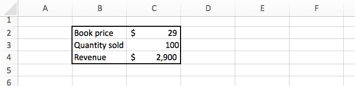
If we sell 100 books at $29 each, we will make $2,900.
The data above assume we know the book price and how many copies we will sell. But we’re actually not sure, so we’d like to know the revenue for different combination of price and quantity. For example: how much profit will we make if we sell 150 copies instead of 100, and what if the price is $19 or $49?
There are 2 main ways to do that:
- Manually change the 2 inputs, and see how the result change.
- Do that automatically with the data table feature.
Nobody likes doing repetitive tasks manually, so let’s try the second option 
The Set Up
Before we start using the data table, we need to do some changes to our data.
First we need to copy the formula to a separate place. You can do this by simply typing =C4 in a blank cell.
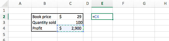
Then we need to tell Excel what values we would like to test. To the right of the formula we list all the prices ($19, $29, $49), and below the formula we list all the quantities (25, 50, 100).
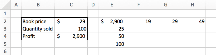
And we can add some basic formatting (borders and currency) to make things look slightly better.
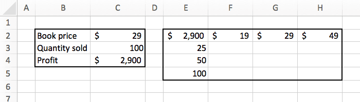
Our goal is to fill this table with the profit for each combination of price and quantity.
Data Table Example
Now we can start the interesting part!
Select the new table we just created, and in the «data» tab, click on the «what if analysis» button. There select «data table».
A popup will appear that you need to fill like this:
- Row input cell: we listed the price at the top, so the «row input» is the price, which is in C2.
- Column input cell»: we listed the quantity in the left, so the «column input» is the quantity, which is in C3.
Press OK, and we are done. Excel did the math for us, and automatically updated the spreadsheet with all the numbers we wanted.
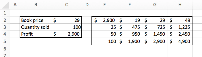
Now we can see exactly how much revenue we will make based on the different combination of inputs. For example it shows that selling 50 copies at $49 will make us $2,450. That’s super powerful.
Limitations
For your information, using data tables have some drawbacks. Here I listed three limitations that make me most uncomfortable:
- The performance and calculation speed of an Excel file will be slowed down if it contains many data tables.
- The structure of the data table is fixed. You will get an error message if you try to insert a row or column in a data table, or if you delete just a single cell in it.
- The data table must be located on the same tab as the setup data table (as mentionned above in the Set Up section). You cannot link the data table to cells on a different tab.
Conclusion
With just a few clicks, we can get Excel to do some magic computation and give us interesting information.
For this example we had a simple formula. But you could do the same on something much more complex, and Excel will give you the perfect answer in no time.