
A data table is a range of cells in which you can change values in some of the cells and come up with different answers to a problem. A good example of a data table employs the PMT function with different loan amounts and interest rates to calculate the affordable amount on a home mortgage loan. Experimenting with different values to observe the corresponding variation in results is a common task in data analysis.
In Microsoft Excel, data tables are part of a suite of commands known as What-If analysis tools. When you construct and analyze data tables, you are doing what-if analysis.
What-if analysis is the process of changing the values in cells to see how those changes will affect the outcome of formulas on the worksheet. For example, you can use a data table to vary the interest rate and term length for a loan—to evaluate potential monthly payment amounts.
Types of what-if analysis
There are three types of what-if analysis tools in Excel: scenarios, data tables, and goal-seek. Scenarios and data tables use sets of input values to calculates possible results. Goal-seek is distinctly different, it uses a single result and calculates possible input values that would produce that result.
Like scenarios, data tables help you explore a set of possible outcomes. Unlike scenarios, data tables show you all the outcomes in one table on one worksheet. Using data tables makes it easy to examine a range of possibilities at a glance. Because you focus on only one or two variables, results are easy to read and share in tabular form.
A data table cannot accommodate more than two variables. If you want to analyze more than two variables, you should instead use scenarios. Although it is limited to only one or two variables (one for the row input cell and one for the column input cell), a data table can include as many different variable values as you want. A scenario can have a maximum of 32 different values, but you can create as many scenarios as you want.
Learn more in the article, Introduction to What-If Analysis.
Create either one-variable or two-variable data tables, depending on the number of variables and formulas that you need to test.
One-variable data tables
Use a one-variable data table if you want to see how different values of one variable in one or more formulas will change the results of those formulas. For example, you can use a one-variable data table to see how different interest rates affect a monthly mortgage payment by using the PMT function. You enter the variable values in one column or row, and the outcomes are displayed in an adjacent column or row.
In the following illustration, cell D2 contains the payment formula, =PMT(B3/12,B4,-B5), which refers to the input cell B3.
Two-variable data tables
Use a two-variable data table to see how different values of two variables in one formula will change the results of that formula. For example, you can use a two-variable data table to see how different combinations of interest rates and loan terms will affect a monthly mortgage payment.
In the following illustration, cell C2 contains the payment formula, =PMT(B3/12,B4,-B5), which uses two input cells, B3 and B4.
Data table calculations
Whenever a worksheet recalculates, any data tables will also recalculate—even if there has been no change to the data. To speed up calculation of a worksheet that contains a data table, you can change the Calculation options to automatically recalculate the worksheet but not the data tables. To learn more, see the section Speed up calculation in a worksheet that contains data tables.
A one-variable data table contain its input values either in a single column (column-oriented), or across a row (row-oriented). Any formula in a one-variable data table must refer to only one input cell.
Follow these steps:
-
Type the list of values that you want to substitute in the input cell—either down one column or across one row. Leave a few empty rows and columns on either side of the values.
-
Do one of the following:
-
If the data table is column-oriented (your variable values are in a column), type the formula in the cell one row above and one cell to the right of the column of values. This one-variable data table is column-oriented, and the formula is contained in cell D2.

If you want to examine the effects of various values on other formulas, enter the additional formulas in cells to the right of the first formula.
-
If the data table is row-oriented (your variable values are in a row), type the formula in the cell one column to the left of the first value and one cell below the row of values.
If you want to examine the effects of various values on other formulas, enter the additional formulas in cells below the first formula.
-
-
Select the range of cells that contains the formulas and values that you want to substitute. In the figure above, this range is C2:D5.
-
On the Data tab, click What-If Analysis > Data Table (in the Data Tools group or Forecast group of Excel 2016).
-
Do one of the following:
-
If the data table is column-oriented, enter the cell reference for the input cell in the Column input cell field. In the figure above, the input cell is B3.
-
If the data table is row-oriented, enter the cell reference for the input cell in the Row input cell field.
Note: After you create your data table, you might want to change the format of the result cells. In the figure, the result cells are formatted as currency.
-
Formulas that are used in a one-variable data table must refer to the same input cell.
Follow these steps
-
Do either of these:
-
If the data table is column-oriented, enter the new formula in a blank cell to the right of an existing formula in the top row of the data table.
-
If the data table is row-oriented, enter the new formula in a empty cell below an existing formula in the first column of the data table.
-
-
Select the range of cells that contains the data table and the new formula.
-
On the Data tab, click What-If Analysis > Data Table (in the Data Tools group or Forecast group of Excel 2016).
-
Do either of the following:
-
If the data table is column-oriented, enter the cell reference for the input cell in the Column input cell box.
-
If the data table is row-oriented, enter the cell reference for the input cell in the Row input cell box.
-
A two-variable data table uses a formula that contains two lists of input values. The formula must refer to two different input cells.
Follow these steps:
-
In a cell on the worksheet, enter the formula that refers to the two input cells.
In the following example—in which the formula starting values are entered in cells B3, B4, and B5, you type the formula =PMT(B3/12,B4,-B5) in cell C2.
-
Type one list of input values in the same column, below the formula.
In this case, type the different interest rates in cells C3, C4, and C5.
-
Enter the second list in the same row as the formula—to its right.
Type the loan terms (in months) in cells D2 and E2.
-
Select the range of cells that contains the formula (C2), both the row and column of values (C3:C5 and D2:E2), and the cells in which you want the calculated values (D3:E5).
In this case, select the range C2:E5.
-
On the Data tab, in the Data Tools group or Forecast group (in Excel 2016), click What-If Analysis > Data Table (in the Data Tools group or Forecast group of Excel 2016).
-
In the Row input cell field, enter the reference to the input cell for the input values in the row.
Type cell B4 in the Row input cell box. -
In the Column input cell field, enter the reference to the input cell for the input values in the column.
Type B3 in the Column input cell box. -
Click OK.
Example of a two-variable data table
A two-variable data table can show how different combinations of interest rates and loan terms will affect a monthly mortgage payment. In the figure here, cell C2 contains the payment formula, =PMT(B3/12,B4,-B5), which uses two input cells, B3 and B4.
When you set this calculation option, no data-table calculations occur when a recalculation is done on the entire workbook. To manually recalculate your data table, select its formulas and then press F9.
Follow these steps to improve calculation performance:
-
Click File > Options > Formulas.
-
In the Calculation options section, under Calculate, click Automatic except for data tables.
Tip: Optionally, on the Formulas tab, click the arrow on Calculation Options, then click Automatic Except Data Tables (in the Calculation group).
You can use a few other Excel tools to perform what-if analysis if you have specific goals or larger sets of variable data.
Goal Seek
If you know the result to expect from a formula, but don’t know precisely what input value the formula needs to get that result, use the Goal-Seek feature. See the article Use Goal Seek to find the result you want by adjusting an input value.
Excel Solver
You can use the Excel Solver add-in to find the optimal value for a set of input variables. Solver works with a group of cells (called decision variables, or simply variable cells) that are used in computing the formulas in the objective and constraint cells. Solver adjusts the values in the decision variable cells to satisfy the limits on constraint cells and produce the result you want for the objective cell. Learn more in this article: Define and solve a problem by using Solver.
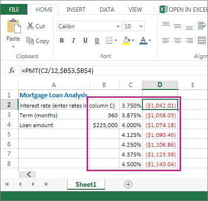
By plugging different numbers into a cell, you can quickly come up with different answers to a problem. A great example is using the PMT function with different interest rates and loan periods (in months) to figure out how much of a loan you can afford for a home or a car. You enter your numbers into a range of cells called a data table.
Here, the data table is the range of cells B2:D8. You can change the value in B4, the loan amount, and the monthly payments in column D automatically update. Using a 3.75% interest rate, D2 returns a monthly payment of $1,042.01 using this formula: =PMT(C2/12,$B$3,$B$4).
You can use one or two variables, depending on the number of variables and formulas you want to test.
Use a one-variable test to see how different values of one variable in a formula will change the results. For example, you can change the interest rate for a monthly mortgage payment by using the PMT function. You enter the variable values (the interest rates) in one column or row, and the outcomes are displayed in a nearby column or row.
In this live workbook, cell D2 contains the payment formula =PMT(C2/12,$B$3,$B$4). Cell B3 is the variable cell, where you can plug in a different term length (number of monthly payment periods). In cell D2, the PMT function plugs in the interest rate 3.75%/12, 360 months, and a $225,000 loan, and calculates a $1,042.01 monthly payment.
Use a two-variable test to see how different values of two variables in a formula will change the results. For example, you can test different combinations of interest rates and number of monthly payment periods to calculate a mortgage payment.
In this live workbook, cell C3 contains the payment formula, =PMT($B$3/12,$B$2,B4), which uses two variable cells, B2 and B3. In cell C2, the PMT function plugs in the interest rate 3.875%/12, 360 months, and a $225,000 loan, and calculates a $1,058.03 monthly payment.
Need more help?
You can always ask an expert in the Excel Tech Community or get support in the Answers community.
What is Data Table in Excel?
A Data Table in Excel helps study the different outputs obtained by changing one or two inputs of a formula. A data table does not allow changing more than two inputs of a formula. However, these two inputs can have as many possible values (to be experimented) as one wants. Excel Data tables, along with Scenarios and Goal Seek are parts of the What-If Analysis tools.
For example, an organization may want to study how changes in the cash possessed impact its working capital. A data table will help the organization know the optimum level of cash (from the specified possible values) to be held to meet its short-term obligations.
The purpose of creating data tables in Excel is to analyze the variation in outputs resulting from a change in the inputs. Moreover, one can have all the outputs in a single table which eases interpretation and allows quick sharing with other users.
Table of contents
- What is Data Table in Excel?
- Types of Data Tables in Excel
- One-Variable Data Table in Excel
- Example #1
- Two-Variable Data Table in Excel
- Example #2
- The Key Points Governing Data Tables in Excel
- Frequently Asked Questions
- Recommended Articles
- One-Variable Data Table in Excel
Types of Data Tables in Excel
The kinds of data tables in Excel are specified as follows:
- One-variable data table
- Two-variable data table
Let us discuss each type of data table one by one with the help of examples.
Note: A data table is different from a regular Excel tableIn excel, tables are a range with data in rows and columns, and they expand when new data is inserted in the range in any new row or column in the table. To use a table, click on the table and select the data range.read more. The former shows the various combinations of inputs and outputs. These outputs are calculated by considering the source dataset as the base. In contrast, an Excel table shows related data that is grouped in one place.
One-Variable Data Table in Excel
A one-variable data tableOne variable data table in excel means changing one variable with multiple options and getting the results for multiple scenarios. The data inputs in one variable data table are either in a single column or across a row.read more is created to study how a change in one input of the formula causes a change in the output. A one-variable data table in excel can be either row-oriented or column-oriented. This implies that all the possible values that an input can assume are listed in either a single row (row-oriented) or a single column (column-oriented) of Excel.
You can download this DATA Table Excel Template here – DATA Table Excel Template
Example #1
There are two images titled “image 1” and “image 2.” The following information is given:
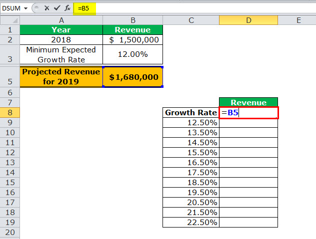
- Image 1 shows an organization’s revenue (in $) for 2018 in cell B2. The minimum growth rate expected is given as 12% in cell B3. The projected revenue (in $ in cell B5) for 2019 has been calculated by using the formula “=B2+(B2*B3).”
- Image 2 shows the possible values (in column C) that the growth rate can assume. The value of cell D8 has been explained in steps 1 and 2 (given further in this example).
We want to perform the following tasks:
- Calculate the projected revenues (in column D) according to the different growth rates (in column C) given in image 2.
- Create a “line with markers” chart showing the growth rates on the x-axis and the projected revenues on the y-axis. Replace the markers of the chart with arrows.
Use a one-variable data table of Excel. Interpret the data table thus created.
Image 1
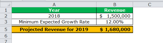
Image 2

The steps for performing the given tasks by using a one-variable data table are listed as follows:
- Enter the data of the two images in Excel. In cell D8, type “equal to” (=) followed by the reference B5. This links cell D8 to cell B5.
The linking of the two cells is shown in the following image.
Since all the growth rates have been entered vertically (C9:C19), our data table is said to be column-oriented. The entire range C8:D19 is our one-variable data table. We are creating a one-variable data table as the change in outputs will be observed against a change in one input, i.e., the growth rate.
Note: Notice that either the formula “=B2+(B2*B3)” could be typed directly in cell D8 or cell D8 can be linked to cell B5. We have chosen to link the two cells.
The linking of cell D8 to cell B5 ensures that any updates in the formula of the latter are automatically reflected in the range D9:D19 of the data table. For instance, if the formula of cell B5 is multiplied by 2 [like =B2+(B2*B3)*2], all the outputs obtained in the range D9:D19 are automatically multiplied by 2.
Had we not linked cells D8 and B5, any changes to the formula of cell B5 would not have changed the value in cell D8. Consequently, the outputs in the range D9:D19 would not have been updated automatically.

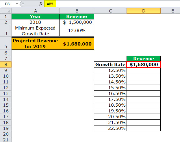
- Press the “Enter” key. Cell D8 shows the value of cell B5, as shown in the following image.
Notice that if one manually enters the value (1680000) in cell D8, the data table will not work. Moreover, one should always type the formula [=B2+(B2*B3)] or link the cell that is one row above and one column to the right of the possible input values (C9:C19). This is the reason we chose to link cell D8 to cell B5.
Note: If the data table is row-oriented, type the formula or link the cell that is one column to the left and one cell below the first possible input value. For instance, had the possible input values been in the range F2:P2, we would have entered the formula or linked cell E3 to cell B5.

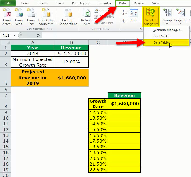
- Select the range of the data table. This selection should include the linked cell (D8), the possible input values (C9:C19), and the empty cells for outputs (D9:D19). Hence, we have selected the range C8:D19, as shown in the following image.

- From the Data tab, click the “what-if analysis” drop-down (in the “data tools” or “forecast” group). Select the option “data table.” This option is shown in the following image.

- The “data table” dialog box opens, as shown in the following image. In the box of “column input cell,” select cell B3, which contains the minimum expected growth rate. As a result, the reference $B$3 appears in this box. Leave the box of “row input cell” blank.
By giving the reference to cell B3 in the “column input cell,” we are telling Excel that at the growth rate of 12%, the projected revenue is $1,680,000. So, with this data table, Excel is being asked the projected revenue when the growth rates vary from 12.5% to 22.5%.
Note 1: A “row input cell” or “column input cell” is a reference to a cell that contains the input. This is the input that can assume the different possible values. Moreover, this input must necessarily be used in the formula whose outputs are to be studied.
In a one-variable data table, either the “row input cell” or the “column input cell” is specified depending on whether the data table is row-oriented or column-oriented.
Note 2: In a one-variable data table, Excel uses either the formula “=TABLE(row_input_cell,)” or “=TABLE(,column_input_cell)” to calculate the different outputs. The former formula is used when the possible input values are in a row, while the latter is used when the possible input values are in a column.
To view the TABLE formula, select any of the output cells and check the formula bar. In this example, the formula “=TABLE(,B3)” is used to calculate the outputs.
Further, Excel uses these TABLE formulas as array formulasArray formulas are extremely helpful and powerful formulas that are used in Excel to execute some of the most complex calculations. There are two types of array formulas: one that returns a single result and the other that returns multiple results.read more. However, these formulas cannot be edited manually, unlike the regular array formulas. But, one can delete all the output cells containing the TABLE formulas.

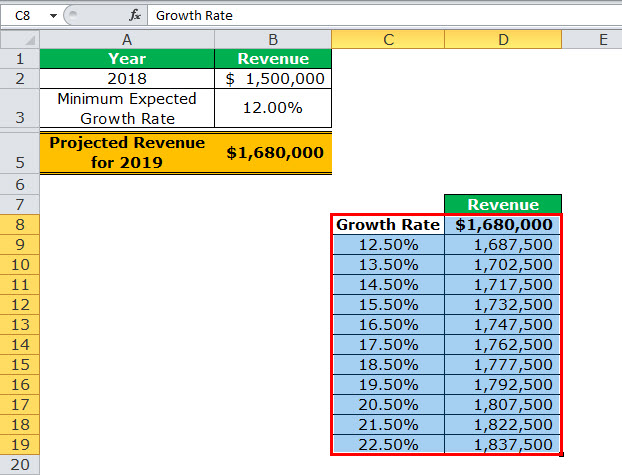
- Click “Ok” in the “data table” window. The range D9:D19 of the data table has been filled with values. The different outputs are shown in the following image.

Interpretation of the one-variable data table: By looking at the data table in the preceding image, one can say that when the growth rate is 12.5%, the projected revenue is $1,687,500. Likewise, when the growth rate is 13.5%, the projected revenue is $1,702,500. Hence, the larger the growth rate, the more the increase in the projected revenue.
The projected revenue is at its maximum ($1,837,500) when the growth rate is at its highest (22.5%). So, the organization can study the variation in outputs when a single input (growth rate) changes.
Note: For more examples related to the one-variable data table of Excel, refer to the hyperlink given before step 1.
- To create a “line with markers” chart that displays the growth rates on the x-axis and the projected revenues on the y-axis, follow the listed steps:
a. Select the range D9:D19 and click the Insert tab on the Excel ribbon.
b. Click the “insert line or area chart” icon from the “charts” group. Select the “line with markers” chart under the 2-D line charts. A “line with markers” chart appears, which displays the projected revenues on the y-axis.
c. Click anywhere on the chart. The “chart tools” menu becomes visible. This menu consists of the Design and Format tabs.
d. Click the Design tab of the “chart tools” menu. Choose “select data” from the “data” group. The “select data source” window opens.
e. Click “edit” under “horizontal (category) axis labels.” The “axis labels” window opens.
f. Select the range C9:C19 in the “axis label range” box. Click “Ok.” Click “Ok” again in the “select data source” window.The “line with markers” chart is created whose x-axis and y-axis look the way they are shown in the image of step 8.
- To replace the default markers of the chart with arrows, follow the listed steps:
a. Select the markers of the chart and right-click them. Choose the “format data series” option from the context menu. The “format data series” pane opens.
b. Click the “fill & line” tab. Expand the “line” tab. In “end arrow type,” select any of the arrows. We have chosen “open arrow.”
c. Select “marker” and expand the “marker options.” Choose the option “none.”
d. Close the “format data series” pane.The “line with markers” chart looks the way it is displayed in the following image. Notice that since the chart shows the projected revenues, we have titled it accordingly.


Two-Variable Data Table in Excel
A two-variable data table in excelA two-variable data table helps analyze how two different variables impact the overall data table. In simple terms, it helps determine what effect does changing the two variables have on the result.read more helps study how changes in two inputs of a formula cause a change in the output. In a two-variable data table, there are two ranges of possible values for the two inputs. From these two ranges, one range is in a row and the other is in a column of Excel.
Example #2
There are three images titled “image 1,” “image 2,” and “image 3.” The following information is given:
- Image 1 shows an organization’s revenue (in $ in 2018) and the minimum growth rate in cells B2 and B3 respectively. Both these figures are the same as that of the previous example. Additionally, the organization gives a 2% discount (in cell B4) to its customers. This is given to boost sales.
- Image 2 shows how the projected revenue (in $ in cell B6) for 2019 has been calculated. The formula “=B2+(B2*B3)-(B2*B4)” is used for this purpose. The amount obtained ($1,650,000) is the projected revenue after the discount.
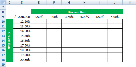
- Image 3 shows the different values in row 9 that the discount rate can assume. The possible values that the growth rate can assume are given in column D. The value of cell D9 has been explained in steps 1 and 2 (given further in this example).
Calculate the projected revenues (in E10:J18) according to the various discount rates (in row 9) and growth rates (in column D). Use a two-variable data table of Excel. Interpret the data table thus created.
Image 1

Image 2
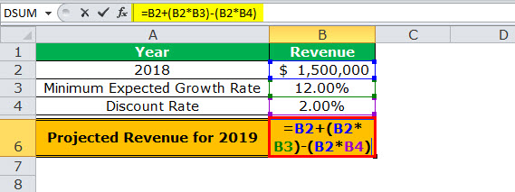
Image 3
The steps for creating a two-variable data table are listed as follows:
Step 1: Enter the data of the preceding images in Excel. In cell D9, type the “equal to” operator followed by the reference B6.
This time we have chosen to link cell D9 to cell B6. Alternatively, we could have also entered the formula [=B2+(B2*B3)-(B2*B4)] in cell D9. This is because, in a two-variable data table, one should type the formula or link the cell that is one column to the left of the first horizontal input value (2.5%). At the same time, this cell should be one row above the first vertical input value (12.5%).
The linking of cells ensures that any changes to the formula of cell B6 are reflected in the value of cell D9. Further, any change in the value of cell D9 will update the outputs (in E10:J18) automatically.
Note: Please ignore the differences in font, colors, and alignment across the images of this example. These differences may be due to the different versions of Excel being used to create the images.

Step 2: Press the “Enter” key. Cell D9 shows the value of cell B6, which is 1,650,000. This is shown in the following image.
The entire range D9:J18 is our two-variable data table. Notice that the excel data table shows the possible discount rates horizontally (in bold in row 9) and the possible growth rates vertically (in column D). This time the variation in outputs resulting from changes in both these inputs (discount rate and growth rate) need to be studied.
Note: If the value is entered manually in cell D9, the excel data table will not work.

Step 3: Select the range D9:J18. Note that the selection should include the linked cell (D9), possible discount rates (E9:J9), possible growth rates (D10:D18), and the empty cells for the outputs (E10:J18).
The selection is shown in the following image.

Step 4: Click the “what-if analysis” drop-down (in the “data tools” or “forecast” group) of the Data tab. Select the option “data table.”
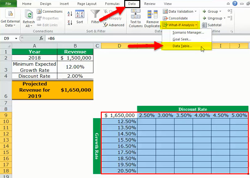
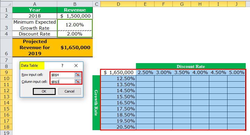
Step 5: The “data table” window opens, as shown in the following image. In the box of “row input cell,” select cell B4. In the box of “column input cell,” select cell B3. The absolute referencesAbsolute reference in excel is a type of cell reference in which the cells being referred to do not change, as they did in relative reference. By pressing f4, we can create a formula for absolute referencing.read more to cells B4 and B3 appear in the two boxes.
Cells B4 and B3 contain the minimum expected growth rate and the discount rate of the source dataset.
By making these selections, Excel is told that at a discount rate of 2% and a growth rate of 12%, the projected revenue is $1,650,000. Therefore, our two-variable data table instructs Excel to calculate the projected revenues when the discount rates and growth rates vary from 2.5% to 5% and 12.5% to 20.5% respectively.
Note: In a two-variable data table, both the “row input cell” and “column input cell” are specified, unlike a one-variable data table where one has to specify either of the two inputs.
Further a two-variable data table uses the formula “=TABLE(row_input_cell,column_input_cell)” to calculate the outputs. So, in this example, the formula “=TABLE(B4,B3)” has been used for the calculations. This formula is visible in the formula bar when an output cell is selected.
For the meaning of the “row input cell” and the “column input cell,” refer to “note 1” under step 5 of example #1.
Step 6: Click “Ok” in the “data table” window. The outputs appear in the range E10:J18, as shown in the following image.

Interpretation of the two-variable data table: When the discount rate is 2.5% and the growth rate is 12.5%, the organization’s projected revenue is $1,650,000 (in cell E10). Notice that this figure is the same as that of cell B6. However, the value in cell B6 takes into account 2% and 12% as the discount rate and growth rate respectively.
Notice that the numbers of cells E10 and B6 match those of cells G11 and I12. This implies that when the discount rate and growth rate are increased in the same proportion (like by 0.5%, 1.5% or 2.5%), the resulting value is the same as the output of the source dataset (in cell B6). Cells E10, G11, and I12 reflect 0.5%, 1.5%, and 2.5% increase in the two rates.
Likewise, had we increased both the discount and growth rates by 1%, the resulting value would have again been $1,650,000. In this case, the discount rate and growth rate would have been 3% and 13% respectively.
By obtaining the projected revenues in the range E10:J18, the organization can sell at an optimum discount rate and, at the same time, target an attainable growth rate. Hence, the organization can choose the most suitable combination of the two rates.
Note: For more examples related to the two-variable data table of Excel, click the hyperlink given before step 1 of this example.
The Key Points Governing Data Tables in Excel
The important points related to data tables of Excel are listed as follows:
- It helps select those input values that fit the business in the best possible manner.
- It facilitates the comparison of the different outputs as all the results are consolidated in one place.
- It presents the results in a tabular format that can neither be edited nor undone with the shortcut “Ctrl+Z.” The outputs can only be deleted by selecting them and pressing the “Delete” key.
- It uses the TABLE array formulas to calculate the outputs. The “row input cell” and the “column input cell” must be selected carefully to get accurate results. Moreover, the input cell or cells must be on the same worksheet as the data table.
- It need not be refreshed, unlike a pivot table. A change in the values or the formula of the source dataset causes the excel data table to update automatically.
Frequently Asked Questions
1. Define a data table and suggest when it should be used in Excel.
A data table helps analyze how a change in one or two inputs of a formula causes a change in the output. The resulting outputs are arranged in a tabular format, making them easy to compare and interpret.
A data table of Excel should be used in the following situations:
• When the outputs resulting from a change in one or two inputs need to be studied
• When the most optimum input value or values need to be chosen
• When all the combinations of inputs and outputs need to be explored in one glance
2. How to create a data table in Excel?
The steps to create a data table in Excel are listed as follows:
a. Enter the source dataset in an Excel worksheet. Use one or two inputs to calculate an output.
b. Arrange the possible values, which an input can assume, in a row and/or column.
c. Link one cell of the data table to the output cell of the source dataset. Alternatively, in a cell of the data table, enter the formula whose outputs need to be studied.
d. Select the data table. The selection should include the linked cell (or the formula cell of the data table), the possible input values, and the empty cells for outputs.
e. Select the “data table” option from the “what-if analysis” drop-down of the Data tab. The “data table” window opens.
f. Enter either the “row input cell” or “column input cell” if the impact of changing one input is to be studied. To study the impact of changing two inputs, enter both “row input cell” and “column input cell.”
g. Click “Ok” in the “data table” window.
A one-variable or two-variable data table is created depending on the execution of steps “a,” “b,” and “f.”
Note: For more details on creating a data table in Excel, refer to the examples of this article.
3. How does a data table work in Excel?
A data table works on the policy “what will be the result if one or two inputs of a formula are changed?” One cell of the data table is linked to the source dataset. In this way, Excel is told how the inputs are to be used in calculating the output.
Next, as the possible input values are supplied, Excel is asked to calculate the outputs using the same formula as that of the source dataset. The resulting table shows the different mixes of inputs and outputs, thereby assisting the user in decision-making.
Recommended Articles
This has been a guide to Data Tables in Excel. Here we discuss how to create one-variable and two-variable data tables along with practical Excel examples. You may learn more about Excel from the following articles–
- Two-Variable Data Table in ExcelA two-variable data table helps analyze how two different variables impact the overall data table. In simple terms, it helps determine what effect does changing the two variables have on the result.read more
- VBA Refresh Pivot TableWhen we insert a pivot table in the sheet, once the data changes, pivot table data does not change itself; we need to do it manually. However, in VBA, there is a statement to refresh the pivot table, expression.refreshtable, by referencing the worksheet.read more
- Merge Tables ExcelWe can use a number of different methods to merge tables in Excel, including the VLOOKUP function, the INDEX function, and the MATCH function.read more
- Data Validation in ExcelThe data validation in excel helps control the kind of input entered by a user in the worksheet.read more
There are some Microsoft Excel features that are awesome but somewhat hidden. And the «data table analysis» is one of them.
Sometimes a formula depends on multiple inputs, and you’d like to see how different inputs values would impact the result. The data table is perfect for that situation.
This is extremely useful to analyze a problem in Excel and figure out the best solution.
The Dataset
To use the data table feature we will need some data.
Here’s a table with 2 inputs (book price and quantity sold), and a formula (revenue = price * quantity).
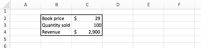
If we sell 100 books at $29 each, we will make $2,900.
The data above assume we know the book price and how many copies we will sell. But we’re actually not sure, so we’d like to know the revenue for different combination of price and quantity. For example: how much profit will we make if we sell 150 copies instead of 100, and what if the price is $19 or $49?
There are 2 main ways to do that:
- Manually change the 2 inputs, and see how the result change.
- Do that automatically with the data table feature.
Nobody likes doing repetitive tasks manually, so let’s try the second option 
The Set Up
Before we start using the data table, we need to do some changes to our data.
First we need to copy the formula to a separate place. You can do this by simply typing =C4 in a blank cell.
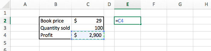
Then we need to tell Excel what values we would like to test. To the right of the formula we list all the prices ($19, $29, $49), and below the formula we list all the quantities (25, 50, 100).
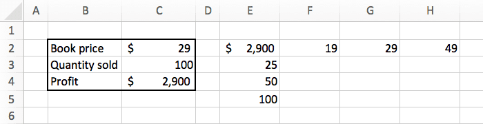
And we can add some basic formatting (borders and currency) to make things look slightly better.
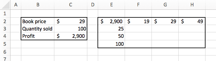
Our goal is to fill this table with the profit for each combination of price and quantity.
Data Table Example
Now we can start the interesting part!
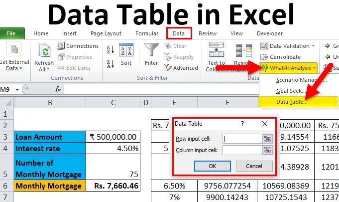
Select the new table we just created, and in the «data» tab, click on the «what if analysis» button. There select «data table».
A popup will appear that you need to fill like this:
- Row input cell: we listed the price at the top, so the «row input» is the price, which is in C2.
- Column input cell»: we listed the quantity in the left, so the «column input» is the quantity, which is in C3.
Press OK, and we are done. Excel did the math for us, and automatically updated the spreadsheet with all the numbers we wanted.
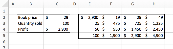
Now we can see exactly how much revenue we will make based on the different combination of inputs. For example it shows that selling 50 copies at $49 will make us $2,450. That’s super powerful.
Limitations
For your information, using data tables have some drawbacks. Here I listed three limitations that make me most uncomfortable:
- The performance and calculation speed of an Excel file will be slowed down if it contains many data tables.
- The structure of the data table is fixed. You will get an error message if you try to insert a row or column in a data table, or if you delete just a single cell in it.
- The data table must be located on the same tab as the setup data table (as mentionned above in the Set Up section). You cannot link the data table to cells on a different tab.
Conclusion
With just a few clicks, we can get Excel to do some magic computation and give us interesting information.
For this example we had a simple formula. But you could do the same on something much more complex, and Excel will give you the perfect answer in no time.
- Таблица данных в Excel
Таблица данных в Excel (Содержание)
- Таблица данных в Excel
- Как создать таблицу данных в Excel?
Таблица данных в Excel
Таблицы данных используются для анализа изменений, которые видны в вашем конечном результате, когда определенные переменные изменяются из вашей функции или формулы. Таблицы данных являются одной из существующих частей инструментов анализа «что, если», которые позволяют наблюдать за результатами, экспериментируя с различными значениями переменных, и сравнивать результаты, сохраненные в таблице данных.
Существует два типа таблиц данных :
- Таблица с одной переменной.
- Таблица двух переменных.
Как создать таблицу данных в Excel?
Таблица данных в Excel очень проста и легка в создании. Давайте разберем работу таблицы данных в Excel на нескольких примерах.
Вы можете скачать этот шаблон таблицы данных Excel здесь — Шаблон таблицы данных Excel
Таблица данных в Excel Пример № 1 — Таблица данных с одной переменной
Таблицы данных с одной переменной эффективны в случае анализа изменений в результате вашей формулы, когда вы изменяете значения для одной входной переменной.
Вариант использования таблицы данных с одной переменной в Excel:
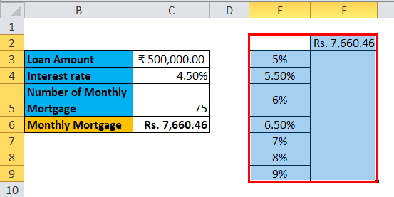
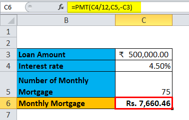
Таблица данных с одной переменной полезна в сценариях, где человек может наблюдать, как различные процентные ставки изменяют сумму их ипотечной суммы, подлежащей выплате. Рассмотрим приведенный ниже рисунок, который показывает сумму ипотеки, рассчитанную на основе процентной ставки с использованием функции PMT.
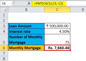
В таблице выше приведены данные, в которых сумма ипотеки рассчитывается на основе процентной ставки, периода ипотеки и суммы кредита. Для расчета ежемесячной суммы ипотеки используется формула PMT, которая может быть записана как = PMT (C4 / 12, C5, -C3).
В случае соблюдения ежемесячной суммы ипотеки для разных процентных ставок, где процентная ставка рассматривается как переменная. Для этого необходимо создать одну таблицу переменных данных. Шаги для создания таблицы данных с одной переменной следующие:
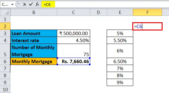
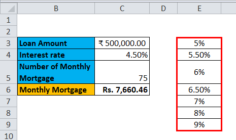
Шаг 1: Подготовьте столбец, который состоит из разных значений для процентных ставок. Мы ввели разные значения для процентных ставок в столбце, который выделен на рисунке.

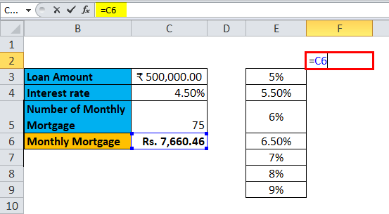
Шаг 2: В ячейке (F2), которая находится на одну строку выше и по диагонали к столбцу, подготовленному вами на предыдущем шаге, введите this = C6.
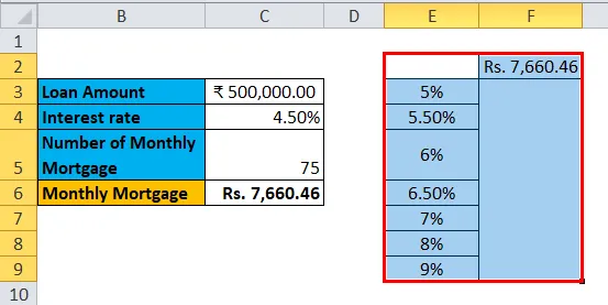
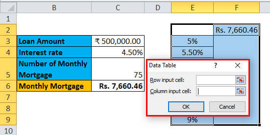
Шаг 3: Выберите весь подготовленный столбец по значениям различных процентных ставок вместе с ячейкой, в которую вы вставили значение, т.е. ячейкой F2.
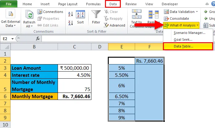
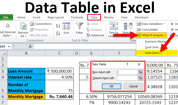
Шаг 4: Нажмите на вкладку «Данные» и выберите «Анализ« что если »», а из раскрывающихся опций выберите «Таблица данных».
Шаг 5: Откроется диалоговое окно таблицы данных.
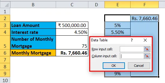
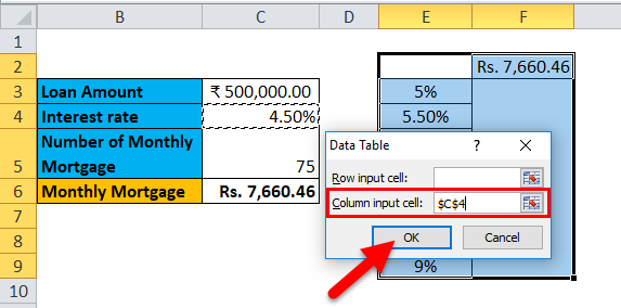
Шаг 6: В ячейке ввода Column обратитесь к ячейке C4 и нажмите OK.
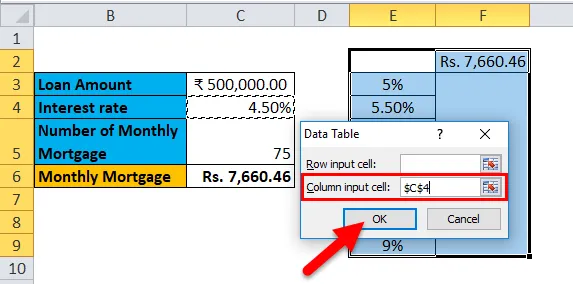
В диалоговом окне мы ссылаемся на ячейку C4 во входной ячейке Column и сохраняем пустую входную ячейку, поскольку мы готовим таблицу данных с одной переменной.
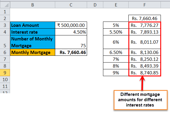
Шаг 7: После выполнения всех шагов мы получаем все разные суммы ипотеки для всех введенных процентных ставок в столбце E (без опознавательных знаков), а разные суммы ипотечных кредитов наблюдаются в столбце F (отмечены).
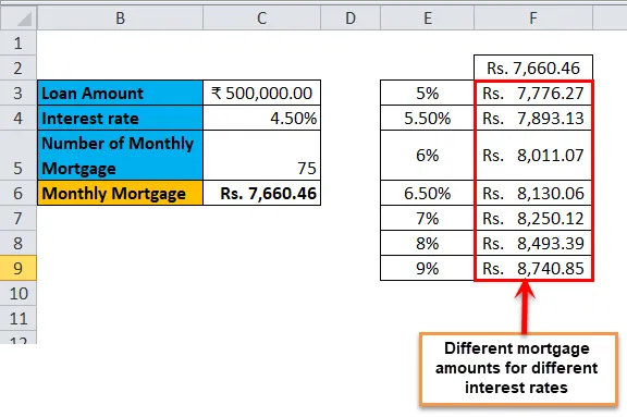
Таблица данных в Excel Пример № 2 — Таблица двух переменных данных
Таблицы данных с двумя переменными полезны в сценариях, где пользователь должен наблюдать изменения в результате их формулы, когда они изменяют две входные переменные одновременно.
Вариант использования таблицы с двумя переменными в Excel:
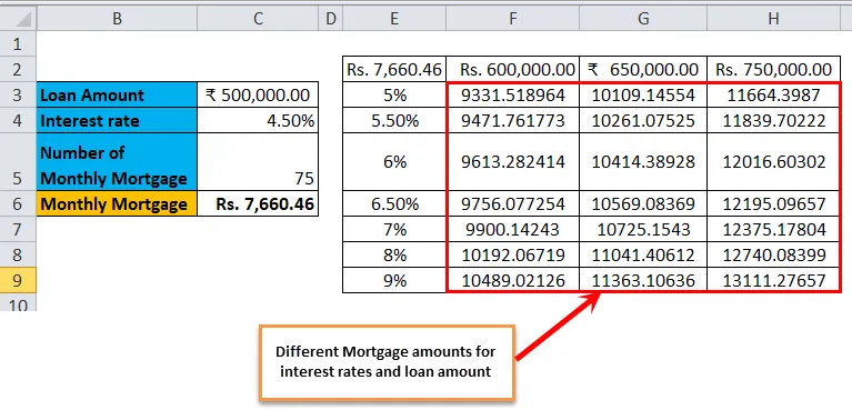
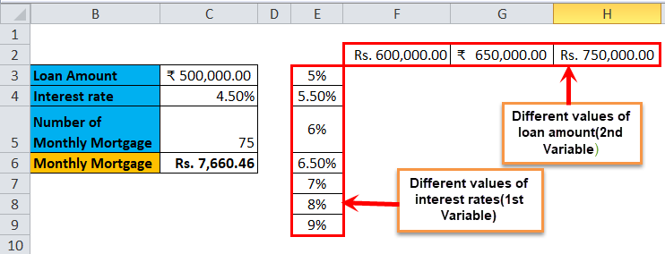
Таблица данных с двумя переменными полезна в сценариях, где человек может наблюдать, как различные процентные ставки и суммы займа изменяют сумму их ипотечной суммы, подлежащей выплате. Вместо того, чтобы рассчитывать отдельные значения отдельно, мы можем наблюдать это с мгновенными результатами. Рассмотрим приведенный ниже рисунок, который показывает сумму ипотеки, рассчитанную на основе процентной ставки с использованием функции PMT.

Приведенный выше пример аналогичен нашему примеру, показанному в предыдущем случае для одной таблицы переменных данных. Здесь сумма ипотеки в ячейке C6 рассчитывается на основе процентной ставки, периода ипотеки и суммы кредита. Для расчета ежемесячной суммы ипотеки используется формула PMT, которая может быть записана как = PMT (C4 / 12, C5, -C3).
Чтобы объяснить таблицу с двумя переменными со ссылкой на приведенный выше пример, мы покажем различные суммы ипотеки и выберем наиболее подходящую для вас, наблюдая за различными значениями процентных ставок и суммы кредита. Для этого необходимо создать таблицу данных с двумя переменными. Шаги для создания таблицы данных с одной переменной следующие:
Шаг 1: Подготовьте столбец, который состоит из разных значений для процентных ставок и суммы кредита.
Мы подготовили столбец, состоящий из разных процентных ставок, и в диагонали ячейки к начальной ячейке столбца мы ввели разные значения суммы кредита.
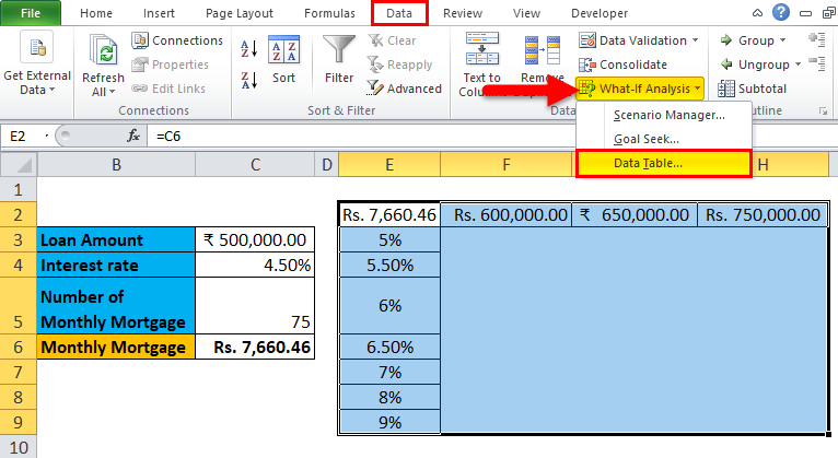
Шаг 2: В ячейке (E2), которая находится на одну строку выше столбца, подготовленного вами на предыдущем шаге, введите this = C6.
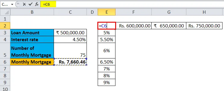
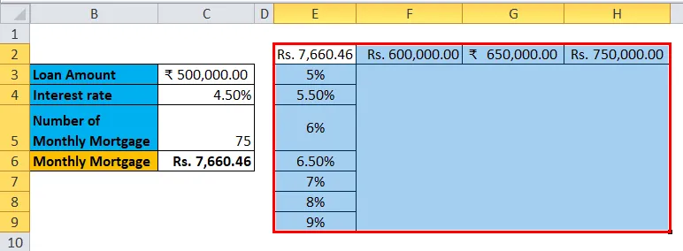
Шаг 3: Выберите весь подготовленный столбец по значениям различных процентных ставок вместе с ячейкой, в которую вы вставили значение, т.е. ячейкой E2.
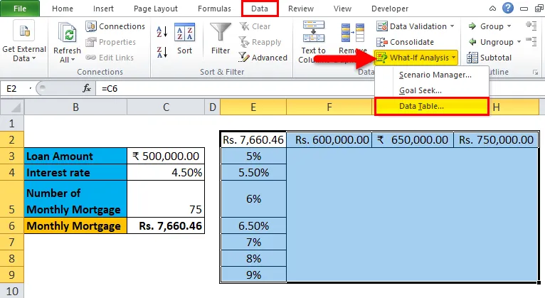
Шаг 4: Нажмите на вкладку «Данные» и выберите «Анализ« что если »», а из раскрывающихся опций выберите «Таблица данных».
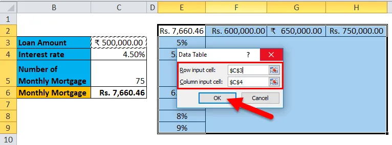
Шаг 5: Откроется диалоговое окно таблицы данных. В «Входной ячейке столбца» см. Ячейку C4 и в «Входной ячейке строки» C3. Оба значения выбираются, так как мы меняем обе переменные и нажимаем ОК.
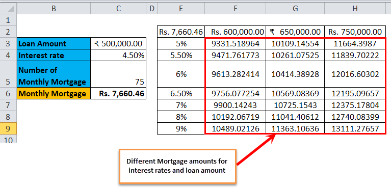
Шаг 6: После выполнения всех шагов мы получаем разные значения сумм ипотеки для разных значений процентных ставок и суммы кредита.
Что нужно помнить о таблице данных в Excel
- Для одной таблицы переменных данных «Ячейка ввода строки» оставлена пустой, а в таблице двух переменных данных заполнены «Ячейка ввода строки» и «Ячейка ввода столбца».
- После того, как анализ «что если» выполнен и значения рассчитаны, вы не сможете изменить или изменить любую ячейку из набора значений.
Рекомендуемые статьи
Это было руководство к таблице данных в Excel. Здесь мы обсуждаем его типы и как создавать примеры таблиц данных и загружаемые шаблоны Excel. Вы также можете посмотреть на эти полезные функции в Excel —
- Руководство по Excel DATEVALUE Функция
- ЧАСТОТА Excel Функция, которую вы должны знать
- Как использовать функцию прогноза Excel?
- Функция COUNTIF Microsoft Excel
Data Table in Excel (Table of Contents)
- Data Table in Excel
- How to Create Data Table in Excel?
Data Table in Excel
Data tables are used to analyze the changes seen in your final result when certain variables are changed from your function or formula. Data tables are one of the existing parts of What-If analysis tools, which allow you to observe your result by experimenting it with different values of variables and to compare the outcomes stored by the data table.
There are two types of a data table, which are as follows:
- One-Variable Data Table.
- Two-Variable Data Table.
How to Create Data Table in Excel?
Data Table in Excel is very simple and easy to create. Let’s understand the working of the Data Table in Excel by Some Examples.
You can download this Data Table Excel Template here – Data Table Excel Template
Data Table in Excel Example #1 – One-Variable Data Table
One-variable data tables are efficient in the case of analyzing the changes in the result of your formula when you change the values for a single input variable.
Use case of One-Variable Data Table in Excel:
The one-variable data table is useful in scenarios where a person can observe how different interest rates change the amount of their mortgage amount to be paid. Consider the below figure, which shows the mortgage amount calculated based on the interest rate using the PMT function.

The table above shows the data where the mortgage amount is calculated based on the interest rate, mortgage period and loan amount. It uses the PMT formula to calculate the monthly mortgage amount, which can be written as =PMT (C4/12, C5,-C3).
In the case of observing the monthly mortgage amount for different interest rates, where the interest rate is considered as a variable. In order to do this, there is a need for creating a one-variable data table. The steps to create the one-variable data table are as follows:
Step 1: Prepare a column which consists of different values for the interest rates. We have entered different values for interest rates in the column which is highlighted in the figure.
Step 2: In the cell (F2), which is one row above and diagonal to the column which you prepared in the previous step, type this = C6.
Step 3: Select the entire prepared column by values of different interest rates along with the cell where you had inserted the value, i.e. F2 cell.
Step 4: Click on the ‘Data’ tab and select ‘What-If Analysis’, and from the options popped down, select ‘Data Table’.

Step 5: Data table dialog box will appear.
Step 6: In the Column input cell, refer to cell C4 and click OK.
In the dialog box, we refer to the cell C4 in the Column input cell and keep the row input cell empty as we are preparing a data table with one variable.
Step 7: After following all the steps, we get all the different mortgage amounts for all entered interests rates in column E (unmarked), and the different mortgage amounts are observed in column F (marked).
Data Table in Excel Example #2 – Two-Variable Data Table
Two-variable data tables are useful in scenarios where a user needs to observe the changes in the result of their formula when they change two input variables simultaneously.
Use-case of Two-Variable Data Table in Excel:
The two-variable data table is useful in scenarios where a person can observe how different interest rates and loan amounts change the amount of their mortgage amount to be paid. Instead of calculating for individual values separately, we can observe them with instantaneous results. Consider the below figure, which shows the mortgage amount calculated based on the interest rate using the PMT function.
The above example is similar to our example shown in the previous case for a one-variable data table. Here the mortgage amount in cell C6 is calculated based on the interest rate, mortgage period and loan amount. It uses the PMT formula to calculate the monthly mortgage amount, which can be written as =PMT (C4/12, C5,-C3).
In order to explain the two-variable data table with reference to the above example, we will show the different mortgage amounts and choose the best which suits you by observing the different values of interest rates and loan amount. In order to do this, there is a need for creating a two-variable data table. The steps to create the one-variable data table are as follows:
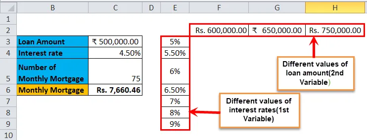
Step 1: Prepare a column which consists of different values for the interest rates and loan amount.
We have prepared a column consisting of the different interest rates, and in the cell diagonal to starting cell of the column, we have entered the different values of the loan amount.
Step 2: In the cell (E2), which is one row above to the column which you prepared in the previous step, type this = C6.

Step 3: Select the entire prepared column by values of different interest rates along with the cell where you had inserted the value, i.e. E2 cell.

Step 4: Click on the ‘Data’ tab and select ‘What-If Analysis’, and from the options popped down, select ‘Data Table’.
Step 5: A Data table dialog box will appear. The ‘Column input cell’ refers to cell C4 and in the ‘Row input cell’ C3. Both the values are selected as we are changing both the variables and Click OK.

Step 6: After following all the steps, we get different values of mortgage amounts for different values of interest rates and loan amount.
Things to Remember About Data Table in Excel
- For one variable data table, the ‘Row input cell’ is left empty, and in a two-variable data table, both ‘Row input cell’ and ‘Column input cell’ are filled.
- Once the What-If analysis is performed, and the values are calculated, you cannot change or modify any cell from the set of values.
Recommended Articles
This has been a guide to a Data Table in Excel. Here we discuss its types and how to create data table examples and downloadable excel templates. You may also look at these useful functions in excel –
- Two-Variable Data Table in Excel
- One Variable Data Table in Excel
- Excel Data Visualization
- Database Function in Excel