
One Variable Data Table | Two Variable Data Table
Instead of creating different scenarios, you can create a data table to quickly try out different values for formulas. You can create a one variable data table or a two variable data table.
Assume you own a book store and have 100 books in storage. You sell a certain % for the highest price of $50 and a certain % for the lower price of $20. If you sell 60% for the highest price, cell D10 below calculates a total profit of 60 * $50 + 40 * $20 = $3800.
One Variable Data Table
To create a one variable data table, execute the following steps.
1. Select cell B12 and type =D10 (refer to the total profit cell).
2. Type the different percentages in column A.
3. Select the range A12:B17.
We are going to calculate the total profit if you sell 60% for the highest price, 70% for the highest price, etc.

4. On the Data tab, in the Forecast group, click What-If Analysis.

5. Click Data Table.

6. Click in the ‘Column input cell’ box (the percentages are in a column) and select cell C4.
We select cell C4 because the percentages refer to cell C4 (% sold for the highest price). Together with the formula in cell B12, Excel now knows that it should replace cell C4 with 60% to calculate the total profit, replace cell C4 with 70% to calculate the total profit, etc.

Note: this is a one variable data table so we leave the Row input cell blank.
7. Click OK.
Result.

Conclusion: if you sell 60% for the highest price, you obtain a total profit of $3800, if you sell 70% for the highest price, you obtain a total profit of $4100, etc.
Note: the formula bar indicates that the cells contain an array formula. Therefore, you cannot delete a single result. To delete the results, select the range B13:B17 and press Delete.
Two Variable Data Table
To create a two variable data table, execute the following steps.
1. Select cell A12 and type =D10 (refer to the total profit cell).
2. Type the different unit profits (highest price) in row 12.
3. Type the different percentages in column A.
4. Select the range A12:D17.
We are going to calculate the total profit for the different combinations of ‘unit profit (highest price)’ and ‘% sold for the highest price’.

5. On the Data tab, in the Forecast group, click What-If Analysis.
6. Click Data Table.
7. Click in the ‘Row input cell’ box (the unit profits are in a row) and select cell D7.
8. Click in the ‘Column input cell’ box (the percentages are in a column) and select cell C4.
We select cell D7 because the unit profits refer to cell D7. We select cell C4 because the percentages refer to cell C4. Together with the formula in cell A12, Excel now knows that it should replace cell D7 with $50 and cell C4 with 60% to calculate the total profit, replace cell D7 with $50 and cell C4 with 70% to calculate the total profit, etc.

9. Click OK.
Result.

Conclusion: if you sell 60% for the highest price, at a unit profit of $50, you obtain a total profit of $3800, if you sell 80% for the highest price, at a unit profit of $60, you obtain a total profit of $5200, etc.
Note: the formula bar indicates that the cells contain an array formula. Therefore, you cannot delete a single result. To delete the results, select the range B13:D17 and press Delete.
Create a Spreadsheet in Excel (Table of Content)
- Introduction to Create Spreadsheet in Excel
- How to Create a Spreadsheet in Excel?
Introduction to Create Spreadsheet in Excel
A spreadsheet is a grid-based file designed to manage or perform any calculation on personal or business data. It is the best choice for users because it has 400+ functions and features such as pivot, coloring, graph, chart, and conditional formatting. It is accessible in both Office 365 and MS Office. Office 365 is a cloud-based application, whereas MS Office is an on-premises solution.
The workbook is the Excel lingo for ‘spreadsheet.’ MS Excel uses this term to emphasize that a single workbook can contain multiple worksheets, each with its own data grid, chart, or graph.
How to Create a Spreadsheet in Excel?
Here are a few examples of creating different types of spreadsheets in Excel with the key features of the created spreadsheets.
You can download this Create Spreadsheet Excel Template here – Create Spreadsheet Excel Template
Example #1 – How to Create Spreadsheet in Excel?
Step 1: Open MS Excel.
Step 2: Go to Menu and select New >> Click on the Blank workbook to create a simple worksheet.
OR – Press Ctrl + N: To create a new spreadsheet.
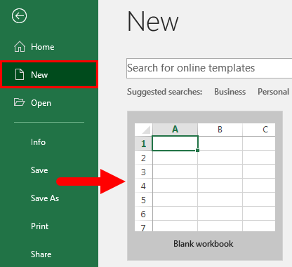
Step 3: By default, Sheet 1 will be created as a worksheet in the spreadsheet. The name of the spreadsheet will be given as Book 1 if you are opening it for the first time.
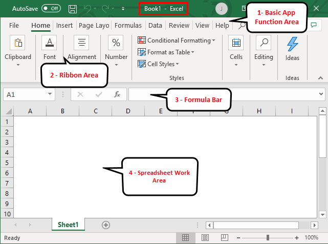
Key Features of the Created Spreadsheet:
- Basic App Functions Area: There is a green banner that contains all types of actions to perform on the worksheet, like – save the file, back or front step move, new, undo, redo, and many more.
- Ribbon Area: This is a gray area just below the basic app functions area called Ribbon. It contains data manipulation, a data visualizing toolbar, page layout tools, and many more.
- Spreadsheet Work Area: By default, a grid contains alphabetic columns like A, B, C, …, Z, ZA…, ZZ, ZZA… and rows as numbers like 1,2 3, …. 100, 101, and… so on. Each rectangle box in the spreadsheet is called a cell, like the one selected in the above image (cell A1). It is a cell where the user can perform their calculation for personal or business data.
- Formula Bar: It shows the data in the selected cell; if it contains any formula, it will show here. Like the above area, a search bar is available in the top right corner, and a sheet tab is available on the downside of the worksheet. A user can change the name of the sheet name.
Once you create an Excel Spreadsheet, you can convert it to a universally accepted format like PDF. For convenience, some useful Excel to PDF converters converts Excel to PDF files for free while maintaining the original formatting.
Example #2 – How to Create a Simple Budget Spreadsheet in Excel?
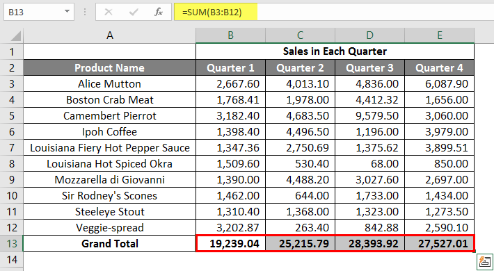
Suppose a user wishes to design a spreadsheet for budget calculation. For 2018, he has a few products and their quarterly sales. He now wants to present his client with this budget.
Let’s see how we can do this with the help of the spreadsheet.
Step 1: Open MS Excel.
Step 2: Go to Menu and select New >> Click on the Blank workbook to create a simple worksheet.
OR – Press Ctrl + N: To create a new spreadsheet.

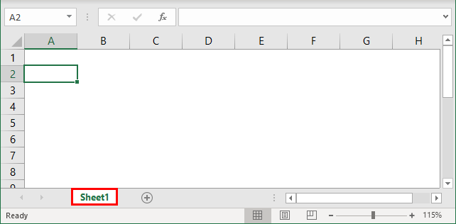
Step 3: Go to the spreadsheet work area, sheet 1.
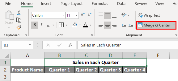
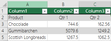
Step 4: Now create headers for Sales in each quarter in the first row by merging cells from B1 to E1. In row 2, give the product name and each quarter’s name.
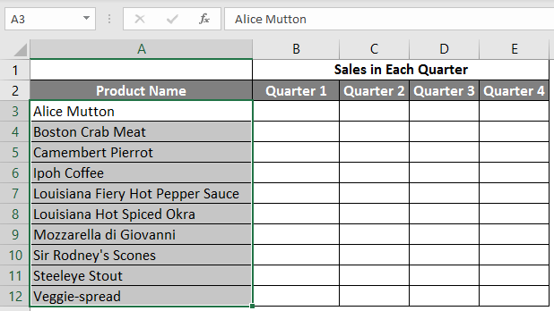
Step 5: Write down all product names in column A.
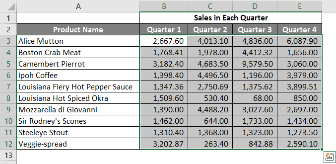
Step 6: Provide the sales data for each quarter before every product.
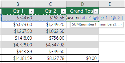
Step 7: In the next row, put one header for Grand Total and calculate each quarter’s total sales.
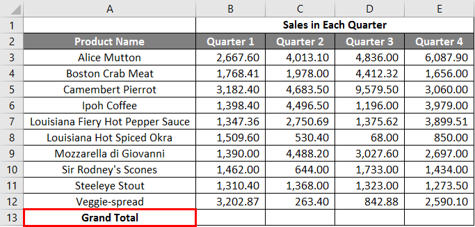
Step 8: Calculate the grand total for each quarter by summation >> apply in other cells in B13 to E13.
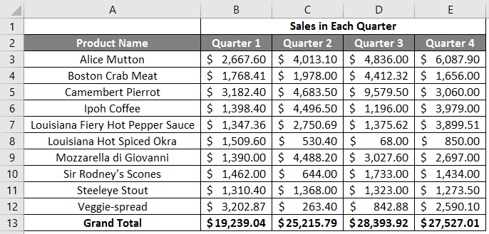
Step 9: Let’s convert the sales value into the ($) currency symbol.
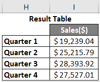
Step 10: Create a Result Table with each quarter’s total sales.
Plot the pie chart to represent the data to the client in a professional way that looks attractive. A user can change the look of the graph by just clicking on it.
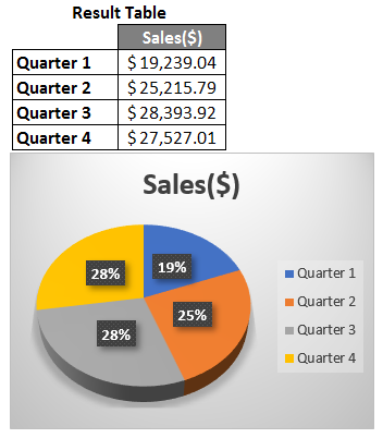
Summary of Example 2: As the user wants to create a spreadsheet to represent sales data to the client, it is done here.
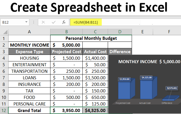
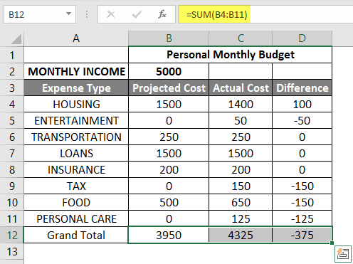
Example #3 – How to Create a Personal Monthly Budget Spreadsheet in Excel?
Let’s assume a user wants to create a spreadsheet to determine their monthly personal budget. For the year 2022, he has estimated costs and actual costs. He now wants to show his family this budget.
Let’s see how we can do this with the help of the spreadsheet.
Step 1: Open MS Excel.
Step 2: Go to Menu and select New >> Click on the Blank workbook to create a simple worksheet.
OR – Press Ctrl + N: To create a new spreadsheet.

Step 3: Go to the spreadsheet work area, Sheet 2.
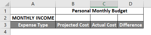
Step 4: Now create headers for Personal Monthly Budget in the first row by merging cells from B1 to D1. In row 2, give MONTHLY INCOME; in row 3, give Expense type, Projected Cost, Actual Cost, and Difference.
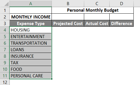
Step 5: Write down all the expenses in column A.
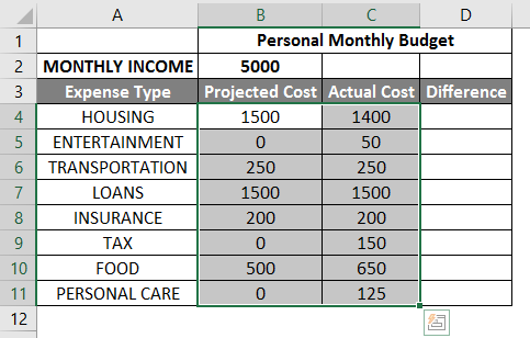
Step 6: Now, provide the monthly income, Projected cost, and Actual Cost data for each expense type.
Step 7: In the next row, put one header for Grand Total and calculate the total and difference from the project to the actual cost.
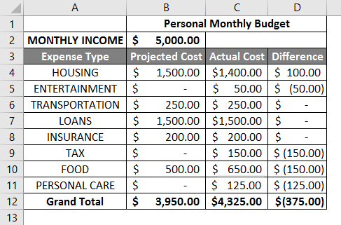
Step 8: Now highlight the header and add boundaries using toolbar graphics. >> The cost and income value in $, so make it by currency symbol.
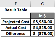
Step 9: Create a Result Table with each quarter’s total sales.
Step 10: Plot the pie chart to represent the data for the family. A user can choose one which he likes.
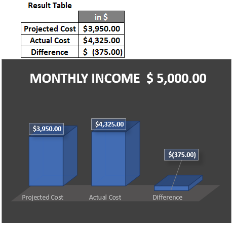
Summary of Example 3: As the user wanted to create a spreadsheet to represent monthly budget data to the family, we have created the same here. The close bracket shows in the data for the negative value.
Things to Remember
- A spreadsheet is a grid-based file designed to manage or perform any calculation on personal or business data.
- It is available in MS Office as well as Office 365.
- The workbook is the Excel lingo for ‘spreadsheet.’ MS Excel uses this term to emphasize that a single workbook can contain multiple worksheets.
How to add data in a spreadsheet Video
Recommended Articles
This article is a comprehensive guide to creating Spreadsheets in Excel. Here we have discussed how to create a Spreadsheet in Excel, examples, and a downloadable Excel template. You may also look at the following articles to learn more –
- Excel Spreadsheet Formulas
- Group Worksheets In Excel
- Excel Spreadsheet Examples
- Worksheets in Excel
What is Data Table in Excel?
A Data Table in Excel helps study the different outputs obtained by changing one or two inputs of a formula. A data table does not allow changing more than two inputs of a formula. However, these two inputs can have as many possible values (to be experimented) as one wants. Excel Data tables, along with Scenarios and Goal Seek are parts of the What-If Analysis tools.
For example, an organization may want to study how changes in the cash possessed impact its working capital. A data table will help the organization know the optimum level of cash (from the specified possible values) to be held to meet its short-term obligations.
The purpose of creating data tables in Excel is to analyze the variation in outputs resulting from a change in the inputs. Moreover, one can have all the outputs in a single table which eases interpretation and allows quick sharing with other users.
Table of contents
- What is Data Table in Excel?
- Types of Data Tables in Excel
- One-Variable Data Table in Excel
- Example #1
- Two-Variable Data Table in Excel
- Example #2
- The Key Points Governing Data Tables in Excel
- Frequently Asked Questions
- Recommended Articles
- One-Variable Data Table in Excel
Types of Data Tables in Excel
The kinds of data tables in Excel are specified as follows:
- One-variable data table
- Two-variable data table
Let us discuss each type of data table one by one with the help of examples.
Note: A data table is different from a regular Excel tableIn excel, tables are a range with data in rows and columns, and they expand when new data is inserted in the range in any new row or column in the table. To use a table, click on the table and select the data range.read more. The former shows the various combinations of inputs and outputs. These outputs are calculated by considering the source dataset as the base. In contrast, an Excel table shows related data that is grouped in one place.
One-Variable Data Table in Excel
A one-variable data tableOne variable data table in excel means changing one variable with multiple options and getting the results for multiple scenarios. The data inputs in one variable data table are either in a single column or across a row.read more is created to study how a change in one input of the formula causes a change in the output. A one-variable data table in excel can be either row-oriented or column-oriented. This implies that all the possible values that an input can assume are listed in either a single row (row-oriented) or a single column (column-oriented) of Excel.
You can download this DATA Table Excel Template here – DATA Table Excel Template
Example #1
There are two images titled “image 1” and “image 2.” The following information is given:
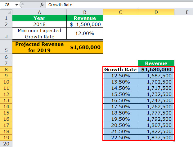
- Image 1 shows an organization’s revenue (in $) for 2018 in cell B2. The minimum growth rate expected is given as 12% in cell B3. The projected revenue (in $ in cell B5) for 2019 has been calculated by using the formula “=B2+(B2*B3).”
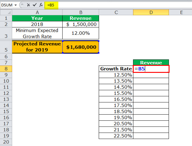
- Image 2 shows the possible values (in column C) that the growth rate can assume. The value of cell D8 has been explained in steps 1 and 2 (given further in this example).
We want to perform the following tasks:
- Calculate the projected revenues (in column D) according to the different growth rates (in column C) given in image 2.
- Create a “line with markers” chart showing the growth rates on the x-axis and the projected revenues on the y-axis. Replace the markers of the chart with arrows.
Use a one-variable data table of Excel. Interpret the data table thus created.
Image 1
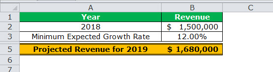
Image 2

The steps for performing the given tasks by using a one-variable data table are listed as follows:
- Enter the data of the two images in Excel. In cell D8, type “equal to” (=) followed by the reference B5. This links cell D8 to cell B5.
The linking of the two cells is shown in the following image.
Since all the growth rates have been entered vertically (C9:C19), our data table is said to be column-oriented. The entire range C8:D19 is our one-variable data table. We are creating a one-variable data table as the change in outputs will be observed against a change in one input, i.e., the growth rate.
Note: Notice that either the formula “=B2+(B2*B3)” could be typed directly in cell D8 or cell D8 can be linked to cell B5. We have chosen to link the two cells.
The linking of cell D8 to cell B5 ensures that any updates in the formula of the latter are automatically reflected in the range D9:D19 of the data table. For instance, if the formula of cell B5 is multiplied by 2 [like =B2+(B2*B3)*2], all the outputs obtained in the range D9:D19 are automatically multiplied by 2.
Had we not linked cells D8 and B5, any changes to the formula of cell B5 would not have changed the value in cell D8. Consequently, the outputs in the range D9:D19 would not have been updated automatically.

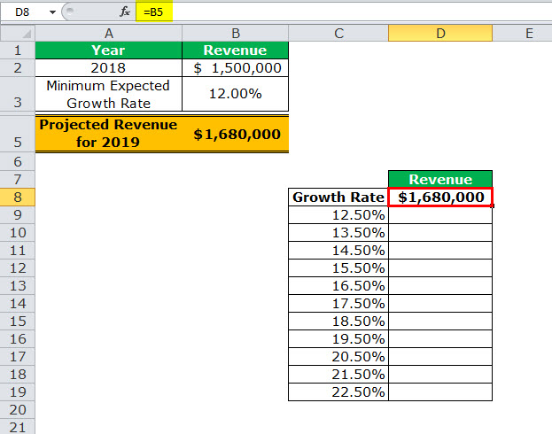
- Press the “Enter” key. Cell D8 shows the value of cell B5, as shown in the following image.
Notice that if one manually enters the value (1680000) in cell D8, the data table will not work. Moreover, one should always type the formula [=B2+(B2*B3)] or link the cell that is one row above and one column to the right of the possible input values (C9:C19). This is the reason we chose to link cell D8 to cell B5.
Note: If the data table is row-oriented, type the formula or link the cell that is one column to the left and one cell below the first possible input value. For instance, had the possible input values been in the range F2:P2, we would have entered the formula or linked cell E3 to cell B5.

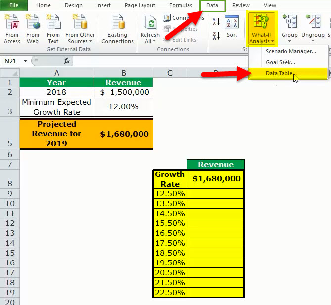
- Select the range of the data table. This selection should include the linked cell (D8), the possible input values (C9:C19), and the empty cells for outputs (D9:D19). Hence, we have selected the range C8:D19, as shown in the following image.

- From the Data tab, click the “what-if analysis” drop-down (in the “data tools” or “forecast” group). Select the option “data table.” This option is shown in the following image.

- The “data table” dialog box opens, as shown in the following image. In the box of “column input cell,” select cell B3, which contains the minimum expected growth rate. As a result, the reference $B$3 appears in this box. Leave the box of “row input cell” blank.
By giving the reference to cell B3 in the “column input cell,” we are telling Excel that at the growth rate of 12%, the projected revenue is $1,680,000. So, with this data table, Excel is being asked the projected revenue when the growth rates vary from 12.5% to 22.5%.
Note 1: A “row input cell” or “column input cell” is a reference to a cell that contains the input. This is the input that can assume the different possible values. Moreover, this input must necessarily be used in the formula whose outputs are to be studied.
In a one-variable data table, either the “row input cell” or the “column input cell” is specified depending on whether the data table is row-oriented or column-oriented.
Note 2: In a one-variable data table, Excel uses either the formula “=TABLE(row_input_cell,)” or “=TABLE(,column_input_cell)” to calculate the different outputs. The former formula is used when the possible input values are in a row, while the latter is used when the possible input values are in a column.
To view the TABLE formula, select any of the output cells and check the formula bar. In this example, the formula “=TABLE(,B3)” is used to calculate the outputs.
Further, Excel uses these TABLE formulas as array formulasArray formulas are extremely helpful and powerful formulas that are used in Excel to execute some of the most complex calculations. There are two types of array formulas: one that returns a single result and the other that returns multiple results.read more. However, these formulas cannot be edited manually, unlike the regular array formulas. But, one can delete all the output cells containing the TABLE formulas.

- Click “Ok” in the “data table” window. The range D9:D19 of the data table has been filled with values. The different outputs are shown in the following image.

Interpretation of the one-variable data table: By looking at the data table in the preceding image, one can say that when the growth rate is 12.5%, the projected revenue is $1,687,500. Likewise, when the growth rate is 13.5%, the projected revenue is $1,702,500. Hence, the larger the growth rate, the more the increase in the projected revenue.
The projected revenue is at its maximum ($1,837,500) when the growth rate is at its highest (22.5%). So, the organization can study the variation in outputs when a single input (growth rate) changes.
Note: For more examples related to the one-variable data table of Excel, refer to the hyperlink given before step 1.
- To create a “line with markers” chart that displays the growth rates on the x-axis and the projected revenues on the y-axis, follow the listed steps:
a. Select the range D9:D19 and click the Insert tab on the Excel ribbon.
b. Click the “insert line or area chart” icon from the “charts” group. Select the “line with markers” chart under the 2-D line charts. A “line with markers” chart appears, which displays the projected revenues on the y-axis.
c. Click anywhere on the chart. The “chart tools” menu becomes visible. This menu consists of the Design and Format tabs.
d. Click the Design tab of the “chart tools” menu. Choose “select data” from the “data” group. The “select data source” window opens.
e. Click “edit” under “horizontal (category) axis labels.” The “axis labels” window opens.
f. Select the range C9:C19 in the “axis label range” box. Click “Ok.” Click “Ok” again in the “select data source” window.The “line with markers” chart is created whose x-axis and y-axis look the way they are shown in the image of step 8.
- To replace the default markers of the chart with arrows, follow the listed steps:
a. Select the markers of the chart and right-click them. Choose the “format data series” option from the context menu. The “format data series” pane opens.
b. Click the “fill & line” tab. Expand the “line” tab. In “end arrow type,” select any of the arrows. We have chosen “open arrow.”
c. Select “marker” and expand the “marker options.” Choose the option “none.”
d. Close the “format data series” pane.The “line with markers” chart looks the way it is displayed in the following image. Notice that since the chart shows the projected revenues, we have titled it accordingly.


Two-Variable Data Table in Excel
A two-variable data table in excelA two-variable data table helps analyze how two different variables impact the overall data table. In simple terms, it helps determine what effect does changing the two variables have on the result.read more helps study how changes in two inputs of a formula cause a change in the output. In a two-variable data table, there are two ranges of possible values for the two inputs. From these two ranges, one range is in a row and the other is in a column of Excel.
Example #2
There are three images titled “image 1,” “image 2,” and “image 3.” The following information is given:
- Image 1 shows an organization’s revenue (in $ in 2018) and the minimum growth rate in cells B2 and B3 respectively. Both these figures are the same as that of the previous example. Additionally, the organization gives a 2% discount (in cell B4) to its customers. This is given to boost sales.
- Image 2 shows how the projected revenue (in $ in cell B6) for 2019 has been calculated. The formula “=B2+(B2*B3)-(B2*B4)” is used for this purpose. The amount obtained ($1,650,000) is the projected revenue after the discount.
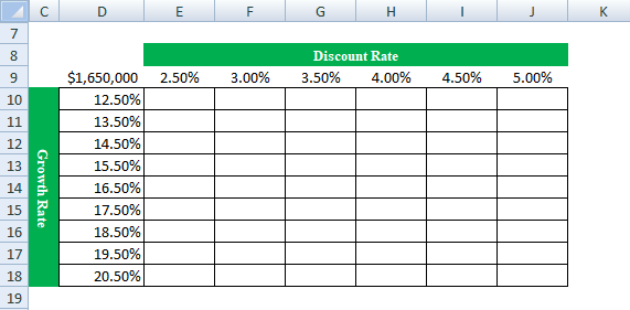
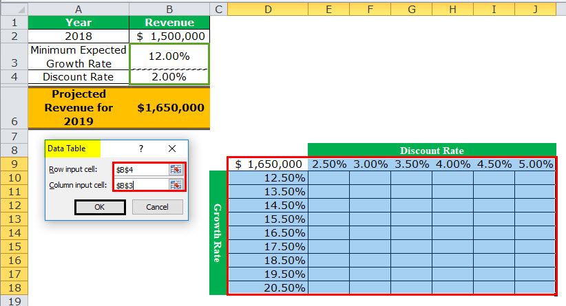
- Image 3 shows the different values in row 9 that the discount rate can assume. The possible values that the growth rate can assume are given in column D. The value of cell D9 has been explained in steps 1 and 2 (given further in this example).
Calculate the projected revenues (in E10:J18) according to the various discount rates (in row 9) and growth rates (in column D). Use a two-variable data table of Excel. Interpret the data table thus created.
Image 1

Image 2
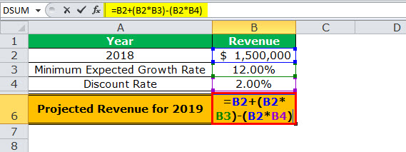
Image 3
The steps for creating a two-variable data table are listed as follows:
Step 1: Enter the data of the preceding images in Excel. In cell D9, type the “equal to” operator followed by the reference B6.
This time we have chosen to link cell D9 to cell B6. Alternatively, we could have also entered the formula [=B2+(B2*B3)-(B2*B4)] in cell D9. This is because, in a two-variable data table, one should type the formula or link the cell that is one column to the left of the first horizontal input value (2.5%). At the same time, this cell should be one row above the first vertical input value (12.5%).
The linking of cells ensures that any changes to the formula of cell B6 are reflected in the value of cell D9. Further, any change in the value of cell D9 will update the outputs (in E10:J18) automatically.
Note: Please ignore the differences in font, colors, and alignment across the images of this example. These differences may be due to the different versions of Excel being used to create the images.

Step 2: Press the “Enter” key. Cell D9 shows the value of cell B6, which is 1,650,000. This is shown in the following image.
The entire range D9:J18 is our two-variable data table. Notice that the excel data table shows the possible discount rates horizontally (in bold in row 9) and the possible growth rates vertically (in column D). This time the variation in outputs resulting from changes in both these inputs (discount rate and growth rate) need to be studied.
Note: If the value is entered manually in cell D9, the excel data table will not work.

Step 3: Select the range D9:J18. Note that the selection should include the linked cell (D9), possible discount rates (E9:J9), possible growth rates (D10:D18), and the empty cells for the outputs (E10:J18).
The selection is shown in the following image.

Step 4: Click the “what-if analysis” drop-down (in the “data tools” or “forecast” group) of the Data tab. Select the option “data table.”
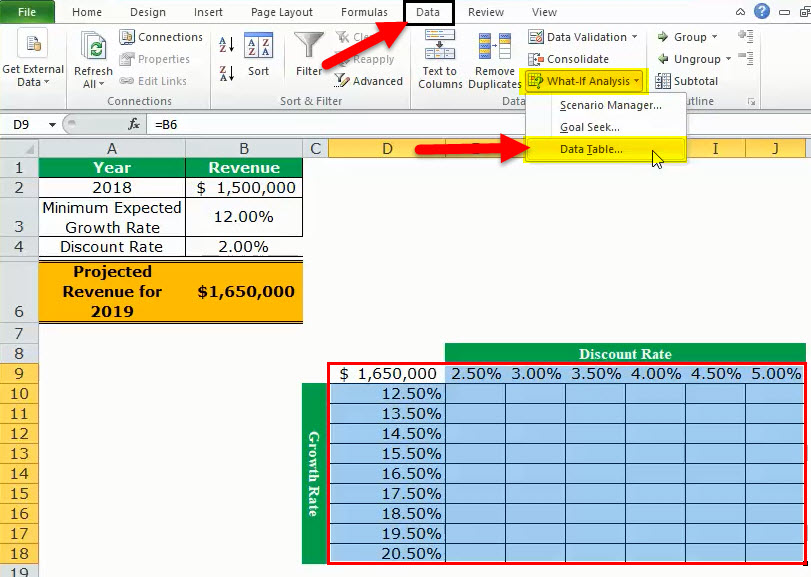
Step 5: The “data table” window opens, as shown in the following image. In the box of “row input cell,” select cell B4. In the box of “column input cell,” select cell B3. The absolute referencesAbsolute reference in excel is a type of cell reference in which the cells being referred to do not change, as they did in relative reference. By pressing f4, we can create a formula for absolute referencing.read more to cells B4 and B3 appear in the two boxes.
Cells B4 and B3 contain the minimum expected growth rate and the discount rate of the source dataset.
By making these selections, Excel is told that at a discount rate of 2% and a growth rate of 12%, the projected revenue is $1,650,000. Therefore, our two-variable data table instructs Excel to calculate the projected revenues when the discount rates and growth rates vary from 2.5% to 5% and 12.5% to 20.5% respectively.
Note: In a two-variable data table, both the “row input cell” and “column input cell” are specified, unlike a one-variable data table where one has to specify either of the two inputs.
Further a two-variable data table uses the formula “=TABLE(row_input_cell,column_input_cell)” to calculate the outputs. So, in this example, the formula “=TABLE(B4,B3)” has been used for the calculations. This formula is visible in the formula bar when an output cell is selected.
For the meaning of the “row input cell” and the “column input cell,” refer to “note 1” under step 5 of example #1.
Step 6: Click “Ok” in the “data table” window. The outputs appear in the range E10:J18, as shown in the following image.

Interpretation of the two-variable data table: When the discount rate is 2.5% and the growth rate is 12.5%, the organization’s projected revenue is $1,650,000 (in cell E10). Notice that this figure is the same as that of cell B6. However, the value in cell B6 takes into account 2% and 12% as the discount rate and growth rate respectively.
Notice that the numbers of cells E10 and B6 match those of cells G11 and I12. This implies that when the discount rate and growth rate are increased in the same proportion (like by 0.5%, 1.5% or 2.5%), the resulting value is the same as the output of the source dataset (in cell B6). Cells E10, G11, and I12 reflect 0.5%, 1.5%, and 2.5% increase in the two rates.
Likewise, had we increased both the discount and growth rates by 1%, the resulting value would have again been $1,650,000. In this case, the discount rate and growth rate would have been 3% and 13% respectively.
By obtaining the projected revenues in the range E10:J18, the organization can sell at an optimum discount rate and, at the same time, target an attainable growth rate. Hence, the organization can choose the most suitable combination of the two rates.
Note: For more examples related to the two-variable data table of Excel, click the hyperlink given before step 1 of this example.
The Key Points Governing Data Tables in Excel
The important points related to data tables of Excel are listed as follows:
- It helps select those input values that fit the business in the best possible manner.
- It facilitates the comparison of the different outputs as all the results are consolidated in one place.
- It presents the results in a tabular format that can neither be edited nor undone with the shortcut “Ctrl+Z.” The outputs can only be deleted by selecting them and pressing the “Delete” key.
- It uses the TABLE array formulas to calculate the outputs. The “row input cell” and the “column input cell” must be selected carefully to get accurate results. Moreover, the input cell or cells must be on the same worksheet as the data table.
- It need not be refreshed, unlike a pivot table. A change in the values or the formula of the source dataset causes the excel data table to update automatically.
Frequently Asked Questions
1. Define a data table and suggest when it should be used in Excel.
A data table helps analyze how a change in one or two inputs of a formula causes a change in the output. The resulting outputs are arranged in a tabular format, making them easy to compare and interpret.
A data table of Excel should be used in the following situations:
• When the outputs resulting from a change in one or two inputs need to be studied
• When the most optimum input value or values need to be chosen
• When all the combinations of inputs and outputs need to be explored in one glance
2. How to create a data table in Excel?
The steps to create a data table in Excel are listed as follows:
a. Enter the source dataset in an Excel worksheet. Use one or two inputs to calculate an output.
b. Arrange the possible values, which an input can assume, in a row and/or column.
c. Link one cell of the data table to the output cell of the source dataset. Alternatively, in a cell of the data table, enter the formula whose outputs need to be studied.
d. Select the data table. The selection should include the linked cell (or the formula cell of the data table), the possible input values, and the empty cells for outputs.
e. Select the “data table” option from the “what-if analysis” drop-down of the Data tab. The “data table” window opens.
f. Enter either the “row input cell” or “column input cell” if the impact of changing one input is to be studied. To study the impact of changing two inputs, enter both “row input cell” and “column input cell.”
g. Click “Ok” in the “data table” window.
A one-variable or two-variable data table is created depending on the execution of steps “a,” “b,” and “f.”
Note: For more details on creating a data table in Excel, refer to the examples of this article.
3. How does a data table work in Excel?
A data table works on the policy “what will be the result if one or two inputs of a formula are changed?” One cell of the data table is linked to the source dataset. In this way, Excel is told how the inputs are to be used in calculating the output.
Next, as the possible input values are supplied, Excel is asked to calculate the outputs using the same formula as that of the source dataset. The resulting table shows the different mixes of inputs and outputs, thereby assisting the user in decision-making.
Recommended Articles
This has been a guide to Data Tables in Excel. Here we discuss how to create one-variable and two-variable data tables along with practical Excel examples. You may learn more about Excel from the following articles–
- Two-Variable Data Table in ExcelA two-variable data table helps analyze how two different variables impact the overall data table. In simple terms, it helps determine what effect does changing the two variables have on the result.read more
- VBA Refresh Pivot TableWhen we insert a pivot table in the sheet, once the data changes, pivot table data does not change itself; we need to do it manually. However, in VBA, there is a statement to refresh the pivot table, expression.refreshtable, by referencing the worksheet.read more
- Merge Tables ExcelWe can use a number of different methods to merge tables in Excel, including the VLOOKUP function, the INDEX function, and the MATCH function.read more
- Data Validation in ExcelThe data validation in excel helps control the kind of input entered by a user in the worksheet.read more
A spreadsheet is a computer application that is designed to add, display, analyze, organize, and manipulate data arranged in rows and columns. It is the most popular application for accounting, analytics, data presentation, etc. Or in other words, spreadsheets are scalable grid-based files that are used to organize data and perform calculations. People all across the world use spreadsheets to create tables for personal and business usage. You can also use the tool’s features and formulas to help you make sense of your data. You could, for example, track data in a spreadsheet and see sums, differences, multiplication, division, and fill dates automatically, among other things. Microsoft Excel, Google sheets, Apache open office, LibreOffice, etc are some spreadsheet software. Among all these software, Microsoft Excel is the most commonly used spreadsheet tool and it is available for Windows, macOS, Android, etc.
A collection of spreadsheets is known as a workbook. Every Excel file is called a workbook. Every time when you start a new project in Excel, you’ll need to create a new workbook. There are several methods for getting started with an Excel workbook. To create a new worksheet or access an existing one, you can either start from scratch or utilize a pre-designed template.
A single Excel worksheet is a tabular spreadsheet that consists of a matrix of rectangular cells grouped in rows and columns. It has a total of 1,048,576 rows and 16,384 columns, resulting in 17,179,869,184 cells on a single page of a Microsoft Excel spreadsheet where you may write, modify, and manage your data.
In the same way as a file or a book is made up of one or more worksheets that contain various types of related data, an Excel workbook is made up of one or more worksheets. You can also create and save an endless number of worksheets. The major purpose is to collect all relevant data in one place, but in many categories (worksheet).
Feature of spreadsheet
As we know that there are so many spreadsheet applications available in the market. So these applications provide the following basic features:
1. Rows and columns: Rows and columns are two distinct features in a spreadsheet that come together to make a cell, a range, or a table. In general, columns are the vertical portion of an excel worksheet, and there can be 256 of them in a worksheet, whereas rows are the horizontal portion, and there can be 1048576 of them.
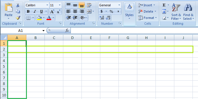
The color light green is used to highlight Row 3 while the color green is used to highlight Column B. Each column has 1048576 rows and each row has 256 columns.
2. Formulas: In spreadsheets, formulas process data automatically. It takes data from the specified area of the spreadsheet as input then processes that data, and then displays the output into the new area of the spreadsheet according to where the formula is written. In Excel, we can use formulas simply by typing “=Formula Name(Arguments)” to use predefined Excel formulas. When you write the first few characters of any formula, Excel displays a drop-down menu of formulas that match that character sequence. Some of the commonly used formulas are:
- =SUM(Arg1: Arg2): It is used to find the sum of all the numeric data specified in the given range of numbers.
- =COUNT(Arg1: Arg2): It is used to count all the number of cells(it will count only number) specified in the given range of numbers.
- =MAX(Arg1: Arg2): It is used to find the maximum number from the given range of numbers.
- =MIN(Arg1: Arg2): It is used to find the minimum number from the given range of numbers.
- =TODAY(): It is used to find today’s date.
- =SQRT(Arg1): It is used to find the square root of the specified cell.
For example, you can use the formula to find the average of the integers in column C from row 2 to row 7:
= AVERAGE(D2:D7)
The range of values on which you want to average is defined by D2:D6. The formula is located near the name field on the formula tab.
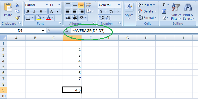
We wrote =AVERAGE(D2:D6) in cell D9, therefore the average becomes (2 + 3 + 4 + 5 + 6 + 7)/6 = 27/6 = 4.5. So you can quickly create a workbook, work on it, browse through it, and save it in this manner.
3. Function: In spreadsheets, the function uses a specified formula on the input and generates output. Or in other words, functions are created to perform complicated math problems in spreadsheets without using actual formulas. For example, you want to find the total of the numeric data present in the column then use the SUM function instead of adding all the values present in the column.
4. Text Manipulation: The spreadsheet provides various types of commands to manipulate the data present in it.
5. Pivot Tables: It is the most commonly used feature of the spreadsheet. Using this table users can organize, group, total, or sort data using the toolbar. Or in other words, pivot tables are used to summarize lots of data. It converts tons of data into a few rows and columns.
Use of Spreadsheets
The use of Spreadsheets is endless. It is generally used with anything that contains numbers. Some of the common use of spreadsheets are:
- Finance: Spreadsheets are used for financial data like it is used for checking account information, taxes, transaction, billing, budgets, etc.
- Forms: Spreadsheet is used to create form templates to manage performance review, timesheets, surveys, etc.
- School and colleges: Spreadsheets are most commonly used in schools and colleges to manage student’s data like their attendance, grades, etc.
- Lists: Spreadsheets are also used to create lists like grocery lists, to-do lists, contact detail, etc.
- Hotels: Spreadsheets are also used in hotels to manage the data of their customers like their personal information, room numbers, check-in date, check-out date, etc.
Components of Spreadsheets
The basic components of spreadsheets are:
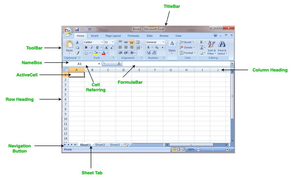
1. TitleBar: The title bar displays the name of the spreadsheet and application.
2. Toolbar: It displays all the options or commands available in Excel for use.
3. NameBox: It displays the address of the current or active cell.
4. Formula Bar: It is used to display the data entered by us in the active cell. Also, this bar is used to apply formulas to the data of the spreadsheet.
5. Column Headings: Every excel spreadsheet contains 256 columns and each column present in the spreadsheet is named by letters or a combination of letters.
6. Row Headings: Every excel spreadsheet contains 65,536 rows and each row present in the spreadsheet is named by a number.
7. Cell: In a spreadsheet, everything like a numeric value, functions, expressions, etc., is recorded in the cell. Or we can say that an intersection of rows and columns is known as a cell. Every cell has its own name or address according to its column and rows and when the cursor is present on the first cell then that cell is known as an active cell.
8. Cell referring: A cell reference, also known as a cell address, is a way for describing a cell on a worksheet that combines a column letter and a row number. We can refer to any cell on the worksheet using cell references (in excel formulae). As shown in the above image the cell in column A and row 1 is referred to as A1. Such notations can be used in any formula or to duplicate the value of one cell to another (by using = A1).
9. Navigation buttons: A spreadsheet contains first, previous, next, and last navigation buttons. These buttons are used to move from one worksheet to another workbook.
10. Sheet tabs: As we know that a workbook is a collection of worksheets. So this tab contains all the worksheets present in the workbook, by default it contains three worksheets but you can add more according to your requirement.
Create a new Spreadsheet or Workbook
To create a new spreadsheet follow the following steps:
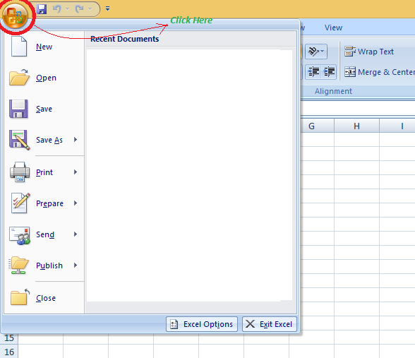
Step 1: Click on the top-left, Microsoft office button and a drop-down menu appear.
Step 2: Now select New from the menu.
Step 3: After selecting the New option a New Workbook dialogue box will appear and then in Create tab, click on the blank Document.
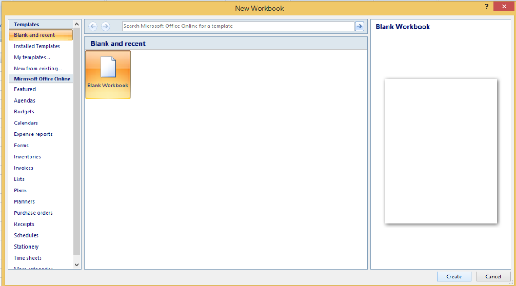
A new blank worksheet is created and is shown on your screen.
Note: When you open MS Excel on your computer, it creates a new Workbook for you.
Saving The Workbook
In Excel we can save a workbook using the following steps:
Step 1: Click on the top-left, Microsoft office button and we get a drop-down menu:
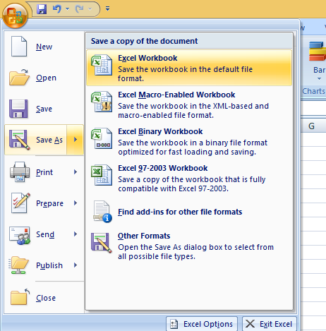
Step 2: Now Save or Save As are the options to save the workbook, so choose one.
- Save As: To name the spreadsheet and then save it to a specific location. Select Save As if you wish to save the file for the first time, or if you want to save it with a new name.
- Save: To save your work, select Save/ click ctrl + S if the file has already been named.
So this is how you can save a workbook in Excel.
Inserting text in Spreadsheet
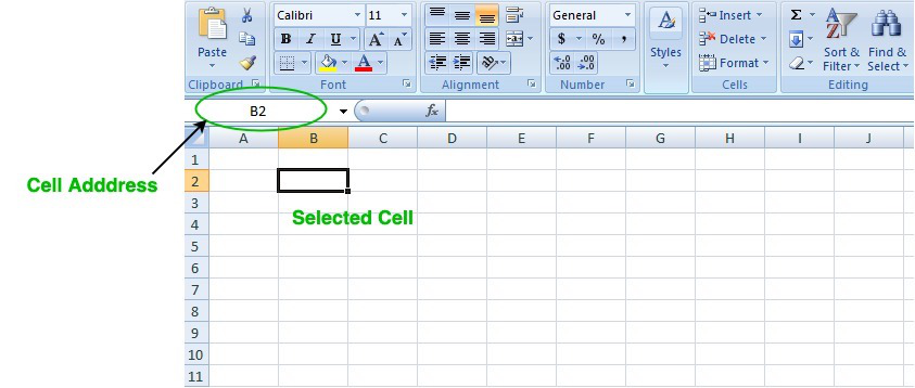
Excel consists of many rows and columns, each rectangular box in a row or column is referred to as a Cell. So, the combination of a column letter and a row number can be used to find a cell address on a worksheet or spreadsheet. We can refer to any cell in the worksheet using these addresses (in excel formulas). The name box on the top left(below the Home tab) displays the cell’s address whenever you click the cell.
To insert the data into the cell follow the following steps:
Step 1: Go to a cell and click on it
Step 2: By typing something on the keyboard, you can insert your data (In that selected cell).
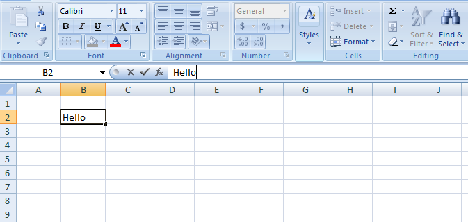
Whatever text you type displays in the formula bar as well (for that cell).
Edit/ Delete Cell Contents in the Spreadsheet
To delete cell content follow the following steps:
Step 1: To alter or delete the text in a cell, first select it.
Step 2: Press the Backspace key on your keyboard to delete and correct text. Alternatively, hit the Delete key to delete the whole contents of a cell. You can also edit and delete text using the formula bar. Simply select the cell and move the pointer to the formula bar.
Excel for Microsoft 365 Excel for Microsoft 365 for Mac Excel 2021 Excel 2021 for Mac Excel 2019 Excel 2019 for Mac Excel 2016 Excel 2016 for Mac Excel 2013 Excel 2010 Excel 2007 More…Less
To make managing and analyzing a group of related data easier, you can turn a range of cells into an Excel table (previously known as an Excel list).

Note: Excel tables should not be confused with the data tables that are part of a suite of what-if analysis commands. For more information about data tables, see Calculate multiple results with a data table.
Learn about the elements of an Excel table
A table can include the following elements:
-
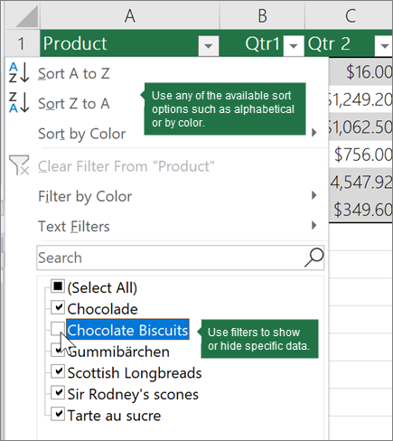
Header row By default, a table has a header row. Every table column has filtering enabled in the header row so that you can filter or sort your table data quickly. For more information, see Filter data or Sort data.

You can turn off the header row in a table. For more information, see Turn Excel table headers on or off.
-
Banded rows Alternate shading or banding in rows helps to better distinguish the data.
-
Calculated columns By entering a formula in one cell in a table column, you can create a calculated column in which that formula is instantly applied to all other cells in that table column. For more information, see Use calculated columns in an Excel table.
-
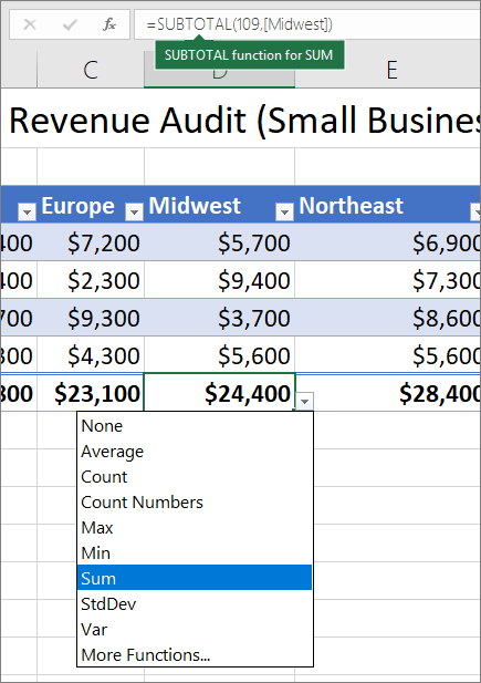
Total row Once you add a total row to a table, Excel gives you an AutoSum drop-down list to select from functions such as SUM, AVERAGE, and so on. When you select one of these options, the table will automatically convert them to a SUBTOTAL function, which will ignore rows that have been hidden with a filter by default. If you want to include hidden rows in your calculations, you can change the SUBTOTAL function arguments.
For more information, also see Total the data in an Excel table.
-
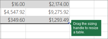
Sizing handle A sizing handle in the lower-right corner of the table allows you to drag the table to the size that you want.
For other ways to resize a table, see Resize a table by adding rows and columns.
Create a table
You can create as many tables as you want in a spreadsheet.
To quickly create a table in Excel, do the following:
-
Select the cell or the range in the data.
-
Select Home > Format as Table.
-
Pick a table style.
-
In the Format as Table dialog box, select the checkbox next to My table as headers if you want the first row of the range to be the header row, and then click OK.
Also watch a video on creating a table in Excel.
Working efficiently with your table data
Excel has some features that enable you to work efficiently with your table data:
-
Using structured references Instead of using cell references, such as A1 and R1C1, you can use structured references that reference table names in a formula. For more information, see Using structured references with Excel tables.
-
Ensuring data integrity You can use the built-in data validation feature in Excel. For example, you may choose to allow only numbers or dates in a column of a table. For more information on how to ensure data integrity, see Apply data validation to cells.
Export an Excel table to a SharePoint site
If you have authoring access to a SharePoint site, you can use it to export an Excel table to a SharePoint list. This way other people can view, edit, and update the table data in the SharePoint list. You can create a one-way connection to the SharePoint list so that you can refresh the table data on the worksheet to incorporate changes that are made to the data in the SharePoint list. For more information, see Export an Excel table to SharePoint.
Need more help?
You can always ask an expert in the Excel Tech Community or get support in the Answers community.
See Also
Format an Excel table
Excel table compatibility issues
Need more help?
Want more options?
Explore subscription benefits, browse training courses, learn how to secure your device, and more.
Communities help you ask and answer questions, give feedback, and hear from experts with rich knowledge.