
Excel for Microsoft 365 Excel for Microsoft 365 for Mac Excel for the web More…Less

To convert to a data type, Excel looks for a match between the cell values and the database provider. If there’s a match, you’ll see a data type icon in the cell to indicate it was converted successfully. If you see a  instead and the Data Selector opens, Excel needs your help to choose the right data type or find a match.
Tip: In Excel for the web, you can select the  Data Type tab or the
  Help tab on the right side to navigate between the panes.
Try it!
-
If you try to convert to a data type and a question mark
 appears instead of the data type icon in the cell, you need to refine or match the result in the Data Selector. If the Data Selector doesn’t automatically open, you can open it by selecting the question mark icon in the cell.
 -
In the Data Selector, review the results and select the one you want. Then the Data Selector will go to the next result that needs identifying.
Note: Need help specifying or getting the correct results? See the section for refining your results below.
-
When all cell values are linked to a data type, the Data Selector will close and you can now view cards and insert data.
Common questions about the Data Selector
How do I refine my results to get the correct data type?
If you selected Automatic to convert text to a data type, Excel will convert to the data type that is the most likely result or display results in the Data Selector that seem most likely. However if incorrect, you can easily change or specify the data type to what you’re looking for.
Note: For example, the term «Brazil» is most likely to convert to the country, but selecting the Movies data type or searching «Brazil movie» in the Data Selector will display results for the movie Brazil.
Try any of these steps to get the correct data type result:
-
Select the cell you want to change > go to Data > select the appropriate data type in the Data Types gallery in the ribbon.
-
Specify terms if possible, either in the Data Selector or by typing in the cell. For example, entering «honeycrisp apple» instead of «honeycrisp».
Note: If your text was converted to the wrong data type, you can also right-click the cell > Data Types > Change… > select a different result or refine your term in the Data Selector.
What if there’s no results that match what I’m looking for?
If the Data Selector is open but there are no results, try these steps:
-
Check that your text is spelled correctly and that each unique term is in its own cell.
-
Try using similar terms and alternatives. For example, entering «bridge» instead of «overpass».
-
Specify terms if possible either in the Data Selector or by typing in the cell. For example, entering «honeycrisp apple» instead of «honeycrisp».
If you still can’t find any results, you can check what linked data types are available to see if we support this subject yet. For the term that has no matching result, you can either manually add data in or delete the row.
What if there are multiple results with the same name?
This can happen with certain data types, like the Foods data type. You can:
-
Refine your results by entering a more specific term in the text box of the Data Selector.
-
Select the image of a result to open the detail view, then use that information to help you make an informed choice.
Want more?
How to provide feedback about data types
Get chemistry facts with the Chemistry data type
Get nutrition facts with the Foods data type
Linked data types FAQ and tips
What linked data types are available in Excel?
Need more help?
Are you looking for options on how to Import Data and Analysis in Excel 365 and cannot find them anywhere? The reason is that they have moved them in the latest version of Excel. They have their own location in the Data section of the Excel Options dialog box. In order to find out How To Modify The Data Options in Excel 365, just keep on reading this post.

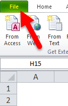
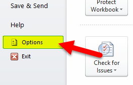
We must select the File tab, in order for us to move to Backstage View and then from the drop-down menu that appears we select the category Options from the left as shown in the image below.

Once the Options command is selected the Excel Options dialog box appears as we can see below. From the left we select the category Data and then from the center of the dialog box where we can Change Options Related To Data Import And Data Analysis

We then locate the Data Options area where underneath we have the following commands in order for us to modify or to activate and deactivate:
-
Make Changes To The Default Layout Of PivotTables:
By selecting this command, we can choose from multiple default layout options for new PivotTables.
-
Disable Undo For Large PivotTables Refresh Operations To Reduce Refresh Time
-
Disable Undo For PivotTables With At Least This Number Of Data Source Rows (In Thousands)
By selecting the Undo operations, we can select the number of rows as a threshold for when to disable it. The default is 300,000 rows.
-
Prefer The Excel Data Model When Creating PivotTables, Query Tables And Data Connections
By selecting this command, the Data Model integrates data from multiple tables, building a relations data source inside an Excel Workbook.
-
Disable Undo For Large Data Model Operations:
-
Disable Undo For Data Model Operations When The Model Is At Least This Large (In MB):
By selecting the Undo operations, we can select the number o Megabytes in file size as a threshold for when to disable it. The default is 8 Mb.
-
Enable Data Analysis Add-Ins: Power Pivot, Power View And 3D Maps:
By selecting this command, we enable the Data Analysis Add-ins, instead of using the Add-ins tab.
-
Disable Automatic Grouping Of Date/Time Columns In Pivot Tables:
By selecting this command, we disable the default of grouping date and time columns with plus (+) signs next to them.

All we need to do is to activate or deactivate the check boxes at the left of the commands or modify the up and down arrows in order to change their defaults. Once we have done all the adjustment we press the Ok button which is located at the bottom right corner of the Excel Options dialog box, in order for them to take place and for us to return to our Workbook.
In my next post I will describe how to Turn On The Legacy Wizards In Microsoft Excel 365, command which is also available in the Data Options dialog box.
Below you can check out the video describing How To Modify the Data Options in Excel 365.
Don’t forget to Subscribe to My YouTube Channel.


About Smart Office — philippospan
MVP:
Honored with the MVP (Most Valuable Professional) for OFFICE SYSTEM title for the years 2011, 2012, 2013, 2014 and 2015 by Microsoft, for my contribution and commitment to the technical communities worldwide.
Microsoft Master Specialist:
This certification provides skill-verification tools that not only help assess a person’s skills in using Microsoft Office programs but also the ability to quickly complete on-the-job tasks across multiple programs in the Microsoft Office system
Posted on June 11, 2018, in Excel 365 English, Microsoft Office 365 ProPlus English and tagged 3D-Maps, Analysis, backstage view, Change Options Related To Data Import And Data Analysis, Data Analysis Add-ins, Data Model, Disable Automatic Grouping Of Date/Time Columns In Pivot Tables, Disable Undo For Large PivotTables, Enable Data Analysis Add-Ins, Excel Options, Excel Workbook, Import Data, Large Data Model Operations, Make Changes To The Default Layout Of PivotTables, Microsoft Excel 365, Microsoft Office 365, Modify The Data Options in Excel 365, Office System, Power Pivot, Power View, Prefer The Excel Data Model, Smart Office, Subscribe, Turn On The Legacy Wizards In Microsoft Excel 365, YouTube Channel. Bookmark the permalink. Comments Off on Modify The Data Options in Excel 365.
Sorting data in Excel has been made quite easy with all the in-built options.
You can easily sort your data alphabetically, based on the value in the cells, or by cell and font color.
You can also do multi-level column sorting (i.e., sorting by column A and then by column B) as well as sorting rows (from left to right).
And if that was not enough, Excel also allows you to create your own custom lists and sort based on that too (how cool is that). So you can sort data based on shirt sizes (XL, L, M, S) or responses (strongly agree, agree, disagree) or intensity (high, medium, low)
Bottom line – there are just too many sorting options you have at your disposal when working with Excel.
And in this massive in-depth tutorial, I will show you all these sorting options and some cool examples where these can be useful.
Since this a huge tutorial with many topics, I am providing a table of content below. You can click on any of the topics and it will instantly take you there.
Accessing the Sorting Options in Excel
Since sorting is such a common thing needed when working with data, Excel provides a number of ways for you to access the sorting options.
Sorting Buttons in the Ribbon
The fastest way to access sorting options is by using the sorting buttons in the ribbons.
When you click on the Data tab in the ribbon, you will see the ‘Sort & Filter’ options. The three buttons on the left in this group is for sorting the data.

The two small buttons allow you to sort your data as soon as you click on these.
![]()
For example, if you have a data set of names, you can just select the entire dataset and click on any of the two buttons to sort the data. The A to Z button sorts the data alphabetically lowest to highest and the Z to A button sorts the data alphabetically highest to lowest.
This buttons also work with numbers, dates or times.
Personally, I never use these buttons as these are limited in what these can do, and there are more chances of errors when using these. But in case you need a quick sort (where there are no blank cells in the dataset), these can be a fast way to do it.
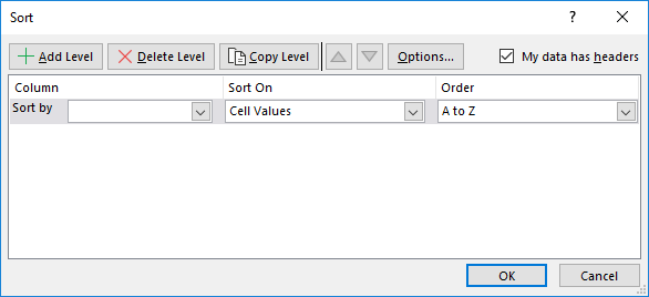
Sorting Dialog Box
In the Data tab in the ribbon, there is another Sort button icon within the sorting group.

When you click this Sort button icon, it opens the sorting dialog box (something as shown below).
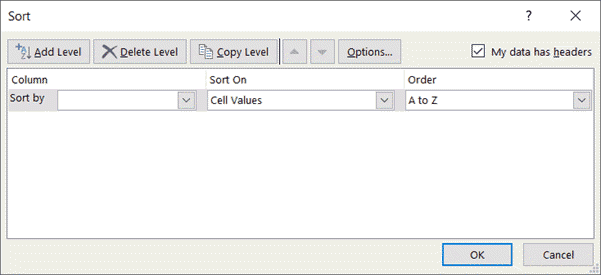
Sorting dialog is the most complete solution for sorting in Excel. All the sorting related options can be accessed through this dialog box.
All the other methods of using sorting options are limited and don’t offer full functionality.
This is the reason I always prefer using the dialog box when I have to sort in Excel.
A major reason for my preference is that there is very less chance of you going wrong when using the dialog box. Everything is well structured and marked (unlike buttons in the ribbon where you may get confused which one to use).
In this tutorial, you’ll find me mostly using the dialog box to sort the data. This is also because some of the things I cover in certain sections (such as multi-level sorting or sorting from left-to-right) can only be done using the dialog box.
Keyboard Shortcut – If you need to sort data often in Excel, I recommend you learn the keyboard shortcut to open the sort dialog box. It’s ALT + A + S + S
Sorting Options in the Filter Menu
If you have applied filters to your dataset, you can also find the sorting options along with the filter options. A filter can be applied by selecting any cell in the dataset, clicking on the Data tab and clicking in the Filter icon.
![]()
Suppose you have a dataset as shown below and you have the filter applied.

When you click on the filter icon for any column (it’s the small downward pointing triangle icon at the right of the column header cell), you’ll see some of the sorting options there as well.

Note that these sorting options change based on the data in the column. So if you have text, it will show you the option to sort from A to Z or Z to A, but if you have numbers, it will show you options to sort from largest to smallest or smallest to largest.
Right-click options
Apart from using the dialog box, using right-click is another method that I sometimes use (it’s also super fast as it only takes two clicks).
When you have a dataset that you want to sort, right-click on any cell and it will show you the sorting options.

Note that you see some options that you don’t see in the ribbon or in the Filter options. While there is the usual sort by value and custom sort option (which opens the Sort dialog box), you can also see options such as Put selected Cell color/Font color/Formatting icon on the top.
I find this option quite useful as it allows me to quickly get all the colored cells (or cells with a different font color) together at the top. I often have the monthly expense data that I go through and highlight some cells manually. I can then use this option to quickly get all these cells together at the top.
Now that I have covered all the ways to access sorting options in Excel, let’s see how to use these to sort data in different scenarios.
Also read: How to Undo Sort in Excel (Revert to Original)
Sorting Data in Excel (Text, Numbers, Dates)
Caveat: Most of the times, sorting works even when you select a single cell in the dataset. But in some cases, you may end up with issues (when you have blank cells/rows/columns in your dataset). When sorting data, it’s best to select the entire data set and then sort it – just to avoid any chance of issues.
Based on the type of data you have, you can use the sorting options in Excel.
Sorting by Text
Suppose you have a dataset as shown below and you want to sort all these records based on the name of the student in alphabetical order.

Below are the steps to sort this text data in alphabetical order:
- Select the entire dataset
- Click the Data tab
- Click the Sort icon. This will open the Sort dialog box.

- In the Sort dialog box, make sure my data has headers is selected. In case your data doesn’t have headers, you can uncheck this.

- In the ‘Sort by’ drop-down, select ‘Name’
- In the ‘Sort On’ drop-down, make sure ‘Cell Values’ is selected
- In the Order drop-down, select A-Z
- Click OK.


The above steps would sort the entire dataset and give the result as shown below.

Why not just use the buttons in the ribbon?
The above method of sorting data in Excel may look like a lot of steps, as compared to just clicking the sort icon in the ribbon.
And this is true.
The above method is longer, but there is no chance of any error.
When you use the sort buttons in the ribbon, there are a few things that can go wrong (and this could be hard to spot when you have a large data set.
While I discuss the drawbacks of using the buttons later in this tutorial, let me quickly show you what can go wrong.
In the below example, since Excel cannot recognize that there is a header row, it sorts the entire dataset, including the header.
![]()
This issue is avoided with the sort dialog box as it explicitly gives you the option to specify whether your data has headers or not.
Since using the Sort dialog box eliminates chances of errors, I recommend you use it instead of all the other sorting methods in Excel
Sorting by Numbers
Now, I am assuming you have already gotten a hang of how text sorting works (covered above this section).
The other types of sorting (such as based on numbers or dates or color) is going to use almost the same steps with minor variations.
Suppose you have a dataset as shown below and you want to sort this data based on the marks scored by each student.

Below are the steps to sort this data based on numbers:
- Select the entire dataset
- Click the Data tab
- Click the Sort icon. This will open the Sort dialog box.
- In the Sort dialog box, make sure my data has headers is selected. In case your data doesn’t have headers, you can uncheck this.
- In the ‘Sort by’ drop-down, select ‘Name’
- In the ‘Sort On’ drop-down, make sure ‘Cell Values’ is selected
- In the Order drop-down, select ‘Largest to Smallest’
- Click OK.
The above steps would sort the entire dataset and give the result as shown below.

Sorting by Date/Time
While the date and time may look different, they are nothing but numbers.
For example, in Excel, the number 44196 would be the date value for 31 December 2020. You can format this number to look like a date, but in the backend in Excel, it still remains a number.
This also allows you to treat dates as numbers. So you can add 10 to a cell with date, and it will give you the number for the date 10 days later.
And the same goes for the time in Excel.
For example, the number 44196.125 represents 3 AM on 31st December 2020. While the integer part of the number represents a full day, the decimal part would give you the time.
And since both date and time are numbers, you can sort these like numbers.
Suppose you have a dataset as shown below and you want to sort this data based on the project submission date.

Below are the steps to sort this data based on the dates:
- Select the entire dataset
- Click the Data tab
- Click the Sort icon. This will open the Sort dialog box.
- In the Sort dialog box, make sure my data has headers is selected. In case your data doesn’t have headers, you can uncheck this.
- In the ‘Sort by’ drop-down, select ‘Submission Date’
- In the ‘Sort On’ drop-down, make sure ‘Cell Values’ is selected
- In the Order drop-down, select ‘Oldest to Newest’
- Click OK.
The above steps would sort the entire dataset and give the result as shown below.

Note that while date and time are numbers, Excel still recognized that these are different in the way it’s displayed. So when you sort by date, it shows ‘Oldest to Newest’ and ‘Newest to Oldest’ sorting criteria, but when you use numbers, it shows ‘Largest to Smallest’ or ‘Smallest to Largest’. Such small things that makes Excel an awesome spreadsheet tool (PS: Google Sheets doesn’t show so much detail, just the bland sort by A-Z or Z-A)
Sorting by Cell Color / Font Color
This option is amazing and I use it all the time (maybe a tad bit too much).
I often have data sets that I analyze manually and highlight cells while I am doing it. For example, I was going through a list of articles on this blog (which I have in an Excel sheet) and I highlighted the ones which I needed to improve.
And once I am done, I can quickly sort this data based on the cell colors. This helps me in getting all these highlighted cells/rows together at the top.
And to add to the awesomeness, you can sort based on multiple colors. So if I highlight cells with article names which need immediate attention in red and some which can be dealt with later with yellow, I can sort the data to show all the red rows first followed by the yellow.
If you’re interested in learning more, I recently wrote this article on sorting based on multiple colors. In this section, I will quickly show you how to sort based on one color only
Suppose you have a dataset as shown below and you want to sort by color and get all the red cells at the top.

Below are the steps to sort by color:
- Select the entire dataset
- Click the Data tab
- Click the Sort icon. This will open the Sort dialog box.
- In the Sort dialog box, make sure my data has headers is selected. In case your data doesn’t have headers, you can uncheck this.
- In the ‘Sort by’ drop-down, select ‘Submission Date’ (or whatever column where you have the colored cells).Since in this example we have colored cells in all the columns, you can choose any.
- In the ‘Sort On’ drop-down, select ‘Cell Color’.
- In the Order drop-down, select the color with which you want to sort. In case you have multiple cell colors in the dataset, it will show you all those colors here
- In the last drop-down, select ‘On Top’. This is where you specify whether you want the colored cells to be on the top of the dataset or at the bottom.
- Click OK.

The above steps would sort your dataset by color and you will get the result as shown below.

Just as we have sorted this data based on the cell color, you can also do it based on the font color and conditional formatting icon.
Multiple Level Data Sorting
In reality, datasets are rarely as simple as the one that I am using in this tutorial.
Yours may extend to thousands of rows and hundreds of columns.
And when you have datasets so big, there is also a need for more data slice and dice. Multiple level data sorting is one of the things you may need when you have a large data set.
Multiple level data sorting means that you can sort the dataset based on values in one column and then sort it again based on values in another column(s).
For example, suppose you have the dataset as shown below and you want to sort this data based on two criteria:
- The region
- The sales

The output of this sorting based on the above two criteria will give you a dataset as shown below.
In the above example, we have the data first sorted by the regions and then within each region, the data is further sorted by the sales value.
This quickly allows us to see which sales reps are doing great in each region or which ones are doing poorly.
Below are the steps to sort the data based on multiple columns:
- Select the entire data set that you want to sort.
- Click the Data tab.
- Click on the Sort Icon (the one shown below). This will open the Sort dialog box.
- In the Sort dialog box, make sure my data has headers is selected. In case your data doesn’t have headers, you can uncheck this.
- In the Sort Dialogue box, make the following selections
- Sort by (Column): Region (this is the first level of sorting)
- Sort On: Cell Values
- Order: A to Z
- Click on Add Level (this will add another level of sorting options).
- In the second level of sorting, make the following selections:
- Then by (Column): Sales
- Sort On: Values
- Order: Largest to Smallest
- Click OK


Pro Tip: The Sort dialog box has a feature to ‘Copy Level’. This quickly copies the selected sorting level and then you can easily modify it. It’s good to know feature and may end up saving you time in case you have to sort based on multiple columns.
Below is a video where I show how to do a multi-level sorting in Excel:
Sorting Based on a Custom List
While Excel already has some common sorting criteria (such as sorting alphabetically with text, smallest to largest or largest to smallest with numbers, oldest to newest or newest to oldest with dates), it may not be enough.
To give you an example, suppose I have the following dataset:

Now, if I sort it based on the region alphabetically, I have two options – A to Z or Z to A. Below is what I get when I sort this data alphabetically from A to Z using the region column.

But what if I want this sort order to be East, West, North, South?
You, of course, can rearrange the data after sorting, but that’s not the efficient way to do this.
The right way to do this would be using custom lists.
A custom list is a list that Excel allows you to create and then use just like the inbuilt lists (such as month names or weekday names). Once you have created a custom list, you can use it in features such as data sorting or fill handle.
Some example where custom lists can be useful include:
- Sorting the data based on region/city name
- Sorting based on T-shirt sizes – Small, Medium, Large, Extra Large
- Sorting based on survey responses – Strongly Agree, Agree, Neutral, Disagree
- Sorting based on probability – high, medium, low
The first step in trying to sort based on the custom criteria is to create the custom list.
Steps to create a custom list in Excel:
- Click the File tab

- Click on Options

- In the Excel Options Dialogue Box, select ‘Advanced’ from the list in the left pane.

- Within Advanced selected, scroll down and select ‘Edit Custom List’.

- In the Custom Lists dialogue box, type your criteria in the box titled List Entries. Type your criteria separated by comma (East, West, North, South) [you can also import your criteria if you have it listed].

- Click Add
- Click OK


Once you have completed the above steps, Excel will create and store a custom list that you can use for sorting data.
Note that the order of the items in the custom list is what determines how your list will be sorted.
When you create a custom list in one Excel workbook, it becomes available to all the workbooks in your system. So you only have to create it once and can reuse it in al workbooks.
Steps to sort using a custom list
Suppose you have the dataset as shown below and you want to sort it based on the regions (the sort order being East, West, North, and South)
Since we have already created a custom list, we can use it to sort our data.
Here are the steps to sort a dataset using a custom list:
- Select the entire dataset
- Click the Data tab
- Click the Sort icon. This will open the Sort dialog box.
- In the Sort dialog box, make sure my data has headers is selected. In case your data doesn’t have headers, you can uncheck this.
- In the ‘Sort by’ drop-down, select ‘Region’ (or whatever column where you have the colored cells)
- In the ‘Sort On’ drop-down, select ‘Cell Values’.
- In the Order drop-down, select ‘Custom List’. As soon as you click on it, it will open the Custom Lists dialog box.
- In the Custom Lists dialog box, select the custom list you have already created from the left pane.
- Click OK. Once you do this, you will see the custom sort criteria in the sort order drop-down field
- Click OK.


The above steps will sort your dataset based on the custom sort criteria.

Note: You don’t have to create a custom list before-hand to sort the data based on it. You can also create it while you’re in the Sort dialog box. When you click on Custom List (in step 7 above), it opens the custom list dialog box. You can create a custom list there as well.
Custom lists are not case sensitive. In case you want to do a case-sensitive sorting, refer to this example.
Also read: How to Sort by Length in Excel? Easy Formulas!
Sorting from Left to Right
While in most cases you’ll likely sort based on the column values, sometimes, you may also have a need to sort based on the row values.
For example, in the below dataset, I want to sort it based on the values in the Region row.

Although this type of data structure is not as common as the columnar data, I have still seen a lot of people working with this kind of construct.
Excel has an in-built functionality that allows you to sort from left to right.
Below are the steps to sort this data from left to right:
- Select the entire dataset (except the headers)
- Click the Data tab
- Click the Sort icon. This will open the Sort dialog box.
- In the Sort dialog box, click on Options.
- In the Sort Options dialog box, select ‘Sort left to right’

- Click OK.
- In the ‘Sort By’ drop-down, select Row 1. By doing this, we are specifying that the sort needs to be done based on the values in Row 1
- In the ‘Sort On’ drop-down, select ‘Cell Values’.
- In the Order drop-down, select A-Z (you can also use custom sort list if you want)
- Click OK.


The above steps would sort the data left to right based on Row 1 values.

Excel doesn’t recognize (or even allow you to specify) the headers when sorting from left to right. So you need to make sure your header cells are not selected when sorting the data. If you select headers cells as well, these will be sorted based on the value in it.
Note: Another way of sorting the data from right to left could be to transpose the data and get it in a columnar form. Once you have it, you can use any of the sorting methods covered so far. Once the sorting is done, you can then copy the resulting data and paste it as transposed data.
Below is a video where I show how to sort data from left to right in Excel
Case Sensitive Sorting in Excel
So far, in all the example above, the sorting has been case independent.
But what if you want to make the sorting case-sensitive.
Thankfully, Excel allows you to specify whether you want the sorting to be case-sensitive or not.
Note: While most of the times you don’t need to worry about case-sensitive sorting, this may be helpful when you get your data from a database such as Salesforce or you manually collate the data and have different people enter the same text in different cases. Having a case sensitive sort may help you keep all the records by the same person/database together.
Suppose you have a dataset as shown below and you want to sort this data based on the region column:

Below are the steps to sort data alphabetically as well as make it case sensitive:
- Select the entire dataset
- Click the Data tab
- Click the Sort icon. This will open the Sort dialog box.
- In the Sort dialog box, make sure my data has headers is selected. In case your data doesn’t have headers, you can uncheck this.
- Click the Options button
- In the Sort Options dialog box, check the ‘Case sensitive’ option
- Click OK.
- In the ‘Sort by’ drop-down, select ‘Region’
- In the ‘Sort On’ drop-down, select ‘Cell Values’.
- In the order drop-down, select A to Z
- Click OK.


The above steps would not only sort the data alphabetically based on the region, but also make it case-sensitive.
You’ll get the resulting data as shown below:

When you sort from A to Z, lower case text is placed above the upper case text.
Getting the Original Sort Order
Often when sorting data in Excel, you may want to go back to the earlier or the original sort order and start afresh,
While you can use the undo functionality in Excel (using Control Z) to go back one step at a time, it may be confusing if you have already done multiple things after sorting the data.
Also, undo works only till you have the workbook open, but when you save and close and it and open it later, you won’t be able to go back to the original sort order.
Here are two simple ways to make sure you don’t lose the original sort order and get it back even after sorting the data:
- Make a copy of the original dataset. This is something I recommend you do even if you don’t need the original sort order. You can have a workbook with all the data and then simply create a copy of the workbook and work on the copy. When I am working on critical datasets, I make a copy every day (with the date or version number as a part of the workbook name).
- Add a column with a series of number. This series of numbers get all mixed up when you sort the data, but in case you want to go back to the original data, you can sort based in this series of numbers.
In this section, let me quickly show you what mean by adding a series and using it to get original sort order back.
Suppose you have a dataset as shown below:

To make sure you have a way to get back this data after sorting it, add a helper column and have a series of numbers in it (as shown below).

Here is a tutorial with different ways to add a column with numbers quickly
When you have the helper column in place, make sure you include it while sorting this dataset.
Suppose I sort this data based on the region and end up getting the data as shown below:

Now, if I want to go back to the original dataset, I can simply sort this data again, but based on the helper column (from low to high).
Simple.. isn’t it?
In case you don’t want the helper column to show, you can either hide it or create a backup and then delete it.
Some Common Issues While Sorting Data in Excel
At the beginning of this article, I showed you different ways to sort data in Excel (including sort buttons in the ribbon, right-click options, filter option, and the sort dialog box).
And to reiterate, using the sort dialog box minimizes the chances or any issues or error that may arise.
Now, let me show you what can go wrong when you use the sort button from the ribbon (the ones shown below)
Not Identifying the Column Headers
Suppose you have a dataset as shown below:
This looks like a decently formatted data set with headers clearly formatted with cell color and bold font.
So when you sort this data based on the names (using the sort buttons in the ribbon), you would expect the header to remain at the top and rest of the data to get sorted.
But what happens when you do it – the header is also considered as normal data and gets sorted (as shown below).
![]()
While Excel is smart enough to recognize headers, in this example, it failed to do so. When using the sort icon buttons in the ribbon, there was no way for you to manually specify that this data has headers.
Note: This issue occurs when I have the dataset and I add and format the headers and sort it. Normally, Excel would be smart enough to identify that there are headers in a dataset (especially when the data type of the header and the data in the column is different). But in this case, it failed to do so when I added the header and sorted right away. If I save this workbook, close it and reopen it, Excel somehow manages to identify the first row and header.
While this may not be an issue in most cases, there is still a chance when you use the sort icons in the ribbon, Using a dialog box eliminates this issue as you can specify that you have headers.
Not Identifying Blank Rows/Columns
This sorting issue is a little more complex – and a lot more common than you would imagine.
Suppose you have a dataset as shown below. Note that row number 6 is hidden (and it’s a blank row).

Now, if I select any cell in the first four rows of the data (the ones above the hidden blank row) and sort this data using the sort icon buttons, it would only sort the first four records on the data set (row 2 to 5). Similarly, if I select any cell in the dataset below the hidden blank row, it will only sort the last seven rows.

And unless you’re looking for it specifically, you’re likely to miss this horrible error.
How to make sure you don’t end up making this sorting error?
To make sure you don’t fall prey to this issue, you need to check your dataset before sorting it.
Select the entire dataset before sorting the data.
You can do that by selecting any cell in the dataset and then using the keyboard shortcut – Control + A.
If there are blank rows/columns in your dataset, the entire dataset won’t get selected. You can identify this by quickly scanning the outline of the selection.
If you see that there is some data left outside the selection, you can manually select it.
To make sure this issue is avoided, it’s best to first unhide all hidden rows and columns and then proceed to sort the data by selecting the entire data set or by first deleting the blank rows.
Partial Sorting (Based on the Last Name)
Sometimes, you may have a dataset that you want to sort based on part of the text.
For example, suppose I have the dataset as shown below and I want to sort this data based on the last name.

To do this, I need to separate this data so that I have only the last names in one column. When I have it, I can use that column to sort the data.
Below is a formula that can give me the last name:
=RIGHT(B2,LEN(B2)-FIND(" ",B2))
This will give you a result as shown below.

Now you can use the Last Name column to sort this data.
Once done, you can delete the last name column or hide it.
Note that the above formula works when you have names that has first and last name only and have no double spaces in between. In case you have names data that is different, you will have to adjust the formula. You can also use Text to Column to quickly split the names based on space character as the delimiter.
This is just one example of sorting based on partial data. Other examples may include sorting based on cities in an address or employee ID based on department codes.
Also, in case the text based on which you need to sort is at the beginning of the text, you can use the normal sort feature only.
Other Sorting Examples (Using Formula and VBA)
So far in this tutorial, I have covered the examples where we have used the in-built sorting functionality in Excel.
Automatically Sorting Using a Formula
When you use the in-built sort functionality and then make any change in the data set, you need to sort it again. The sort functionality is not dynamic.
In case you want to get a dataset that sorts automatically whenever there is any change, you can use the formulas to do it.
Note that to do this, you need to keep the original dataset and the sorted dataset separate (as shown below)

I have a detailed tutorial where I cover how to sort alphabetically using formulas. It shows two methods to do this – using helper columns and using an array formula.
Excel has also introduced the SORT dynamic array formula which can easily do this (without helper column or a complicated array formula). But since this is quite new, you may not have access to it in your version of Excel.
Sorting Using VBA
And finally, if you want to bypass all the sorting dialog box or other sorting options, you can use VBA to sort your data.
In the below example, I have a dataset that sorts the data when I double click on the column header. This makes it easy to sort and can be used in dashboards to make it more user-friendly.
Here is a detailed tutorial where I cover how to sort data using VBA and create something as shown above.
I have tried to cover a lot of examples to show you different ways you can sort data in Excel and all the things you need to keep in mind when doing it.
Hope you found this tutorial useful.
You May Also Like the following Excel Tutorials:
- Search and Highlight Data Using Conditional Formatting
- How to Sort Worksheets in Excel using VBA
- How to Create a Data Entry Form in Excel
- How to Compare Two Columns in Excel
- Excel TRIM Function to Remove Spaces and Clean Data
- Flip Data in Excel | Reverse Order of Data in Column/Row
- How to Shuffle a List of Items/Names in Excel? 2 Easy Formulas!
What is Sort in Excel?
SORT in Excel means arranging the data in a determined order. For example, sometimes we need to place the names alphabetically, sort the numbers from smallest to largest, largest to smallest, dates from oldest to latest, latest to oldest, etc. In Excel, we have a built-in tool called the “SORT” option. This “Sort” option can help us sort the data based on the condition we provide.
The “SORT” option in Excel is under the “Data” tab.

- The “SORT” option plays a key role in organizing the data. For example, if the monthly sales data is not in order from Jan to Dec, it may not be a proper organizing way of the data structure.
- Excel “SORT” option will help us solve all kinds of data to make life easy. In this article, we will demonstrate the usages of the “SORT” option in Excel and save a lot of time.
Table of contents
- What is Sort in Excel?
- How to Sort Data in Excel?
- Example #1 – Single Level Data Sorting
- Example #2 – Multi-Level Data Sorting
- Example #3 – Sorting Dates Data
- Things to Remember
- Recommended Articles
- How to Sort Data in Excel?
How to Sort Data in Excel?
You can download this Sort Options Excel Template here – Sort Options Excel Template
Example #1 – Single Level Data Sorting
It will sort the data based on only one column, nothing else.
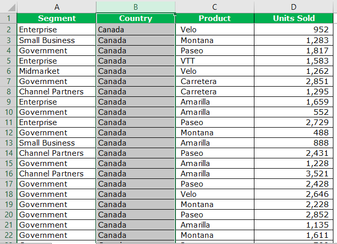
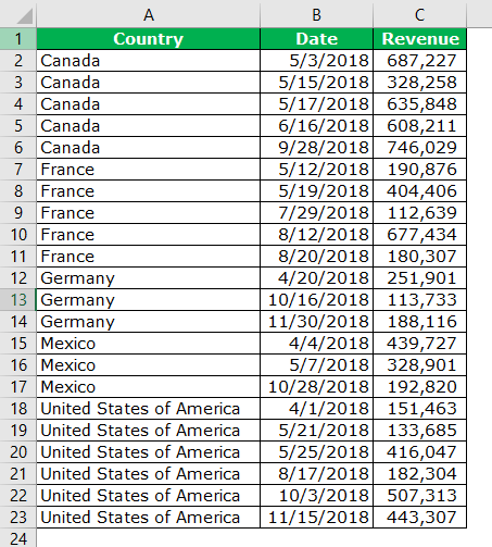
Now, look at the below data. Again, we have sales of different products by segment and country.
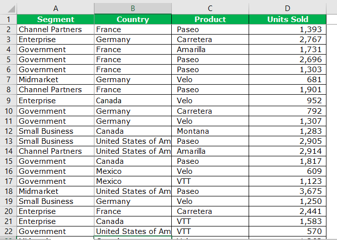
We have the data until the 700th row. Download the Excel file to follow along here.
We want to sort them based on the “Country” column from A to Z.
Below are the steps used for single-level data sorting:
- First, select the data that we want to sort. Next, you can use the shortcut key to select the entire data, select the first row, and then click “Ctrl + Shift + Down Arrow.”

- Go to the “Data” tab > “Sort.” The shortcut key to open the “Sort” option is “ALT + D + S.”

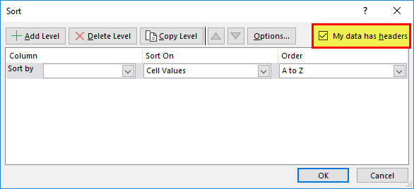
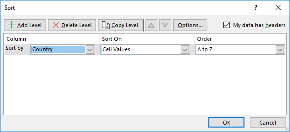
- Make sure the “My data has headers” checkbox has been ticked. If this box has ticked means, the selected data has headers. Otherwise, your header will be treated as the data only.
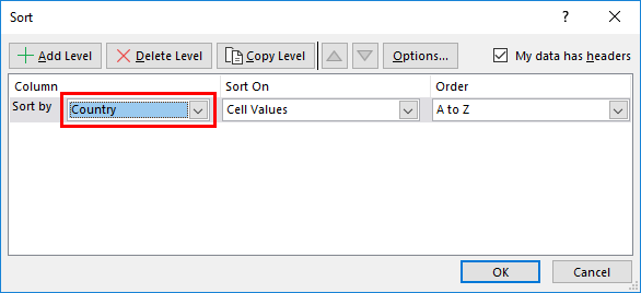
- Click on the “Sort by” dropdown list and select the word “Country.”
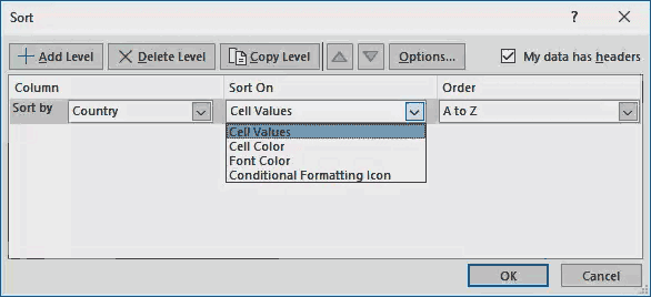
- Click on “Sort On.” Here, we can sort based on values, cell color, font color, and conditional formatting icon.
- Finally, select the “Order.” You can sort A to Z, Z to A, and a custom list here.
- The final “SORT” dialog box should look like this.
- Click on “OK.” It will sort the data country-wise alphabetically from A to Z.


Example #2 – Multi-Level Data Sorting
In the previous example, we have learned single-level sorting. In this example, we will explain the multi-level sorting process.
Previously, we sorted the data country-wise. Assume we want to sort the data segment-wise, product-wise, and units sold from largest to smallest. It requires multi-level sorting.
- Step 1: Select the data. (We are using the same data from the previous example)

- Step 2: Press “ALT + D + S.” (shortcut key to open the SORT box)

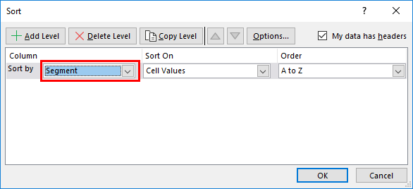
- Step 3: First, select the “Segment” heading.
- Step 4: Click “Add Level” to insert one more layer.

- Step 5: From the second layer, select the “Product.”
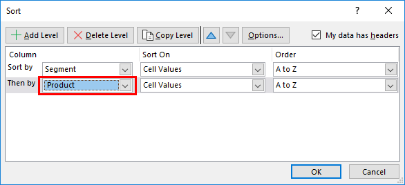
- Step 6: Click “Add Level” to add the third layer.
- Step 7: Select the “Units Sold” header from the third layer.
- Step 8: The “Order” will default to “Smallest to Largest.” Under “Order,” click on the dropdown list and select “Largest to Smallest.”

- Step 9: It will sort the layers alphabetically. It will sort the “Units Sold” column from the largest to the lowest value.

Firstly, it will sort the data based on the “Segment” column. Next, they will sort by “Product” and finally by “Units Sold” (largest to smallest).
Example #3 – Sorting Dates Data
We have a sales table country-wise on different dates. So, we want to sort the data country-wise first and then date-wise (oldest to newest).
- Step 1: Select the data first.
- Step 2: Open the “Sort” option. (ALT + D + S)
- Step 3: Select a “Country” header in the first drop-down list.
- Step 4: Click “Add Level” to insert one more layer.

- Step 5: Select the “Date” header from the second layer.

- Step 6: By default, orders selected “Oldest to Newest.” Our objective is to sort from oldest to newest.
Click on “OK” to sort.
Things to Remember
- We need to select the entire to sort. Otherwise, left-out columns will be as it is.
- Ensure the “My data has headers” check has been selected to sort the data.
- We can sort the colored cells, colored font, etc.
- We also sort the data by applying the filter in excel.
- We can sort from A to Z and Z to A in the case of the alphabet.
- We can sort from “Largest to Smallest” and “Smallest to Largest” in the case of numbers.
- In the case of dates, we can sort from “Oldest to Newest” and “Newest to Oldest.”
Recommended Articles
This article is a guide to Sort in Excel. Here, we will demonstrate the SORT option in Excel (single-level and multi-level sorting) along with an Excel example and a downloadable template. You may also look at these useful functions in Excel: –
- Sort by Number in ExcelWhen a column or a data range in excel has numbers, we can sort the data by numbers in excel. Number filters have various options, the first being largest to smallest or vice versa and the other being conditional formatting options.read more
- Sort by Color in ExcelWhen a column or a data range in excel is formatted with colors either by using the conditional formatting or manually, when we use filter on the data excel provides us with an option to sort the data by color, there is also an option for advanced sort where user can enter different levels of color for sorting.read more
- VBA Sort RangeIn VBA, you can sort a range using the range sort method, which is a property of the range method that allows you to sort a range in order. Header, OrderCustom, MatchCase, Orientation, SortMethod, DataOption1, DataOption2, and DataOption3 are the arguments for this function.read more
- REPT Function in ExcelREPT function is also known as repeat function in excel and as the name suggests this function repeats a given data provided to it to a given number of times so this function takes two arguments one is the text which needs to be repeated and the second argument is the number of times we want the text to be repeated.read more
Reader Interactions
Excel Tool for Data Analysis (Table of Contents)
- Data Analysis Tool in Excel
- Unleash Data Analysis Tool Pack in Excel
- How to Use the Data Analysis Tool in Excel?
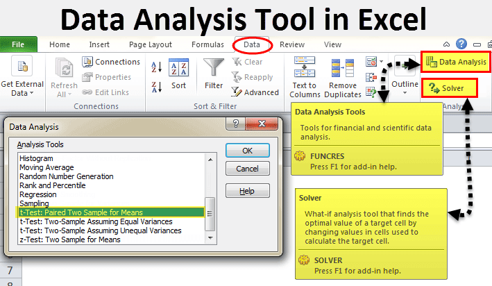
In excel, we have few inbuilt tools which are used for Data Analysis. But these become active only when you select any of them. To enable the Data Analysis tool in Excel, go to the File menu’s Options tab. Once we get the Excel Options window from Add-Ins, select any of the analysis pack, let’s say Analysis Toolpak and click on Go. This will take us to the window from where we can select one or multiple Data analysis tool packs, which can be seen in the Data menu tab.
If you observe excel on your laptop or computer, you may not see the data analysis option by default. You need to unleash it. Usually, a data analysis tool pack is available under the Data tab.
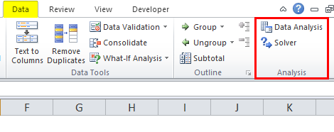
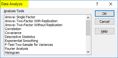
Under the Data Analysis option, we can see many analysis options.
Unleash Data Analysis Tool Pack in Excel
If your excel is not showing this pack, follow the below steps to unleash this option.
Step 1: Go to FILE.
Step 2: Under File, select Options.
Step 3: After selecting Options, select Add-Ins.
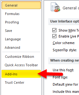
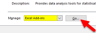
Step 4: Once you click on Add-Ins, at the bottom, you will see Manage drop-down list. Select Excel Add-ins and click on Go.
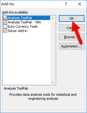
Step 5: Once you click on Go, you will see a new dialogue box. You will see all the available Analysis Tool Pack. I have selected 3 of them and then click on Ok.
Step 6: Now, you will see these options under the Data ribbon.

How to Use the Data Analysis Tool in Excel?
Let’s understand the working of a data analysis tool with some examples.
You can download this Data Analysis Tool Excel Template here – Data Analysis Tool Excel Template
T-test Analysis – Example #1
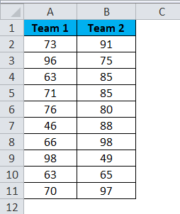
A t-test is returning the probability of the tests. Look at the below data of two teams scoring pattern in the tournament.
Step 1: Select the Data Analysis option under the DATA tab.
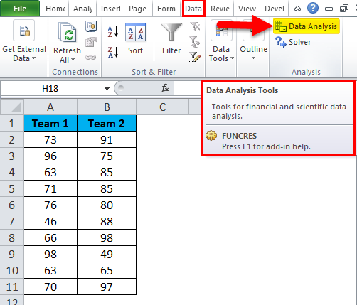
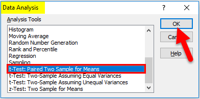
Step 2: Once you click on Data Analysis, you will see a new dialogue box. Scroll down and find the T-test. Under T-test, you will three kinds of T-test; select the first one, i.e. t-Test: Paired Two Sample for Means.
Step 3: After selecting the first t-Test, you will see the below options.
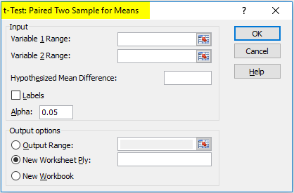
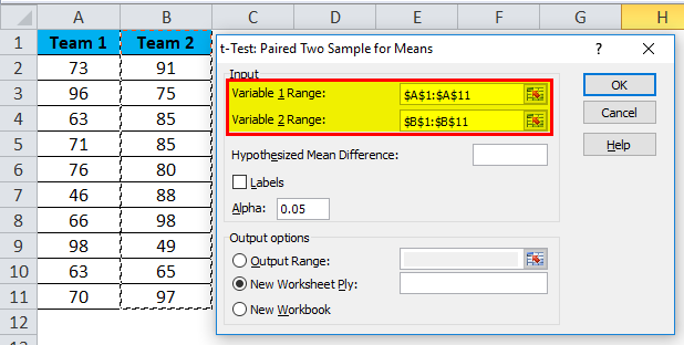
Step 4: Under Variable 1 Range, select team 1 score and under Variable 2 Range, select team 2 score.
Step 5: Output Range selects the cell where you want to display the results.
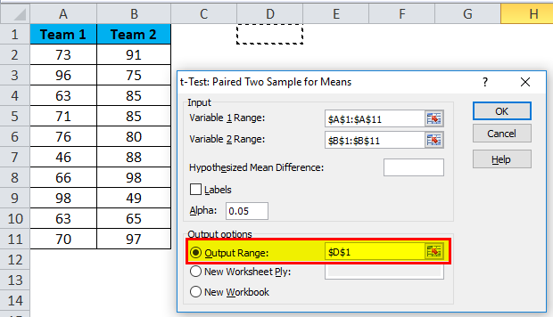
Step 6: Click on Labels because we have selected the ranges, including headings. Click on Ok to finish the test.
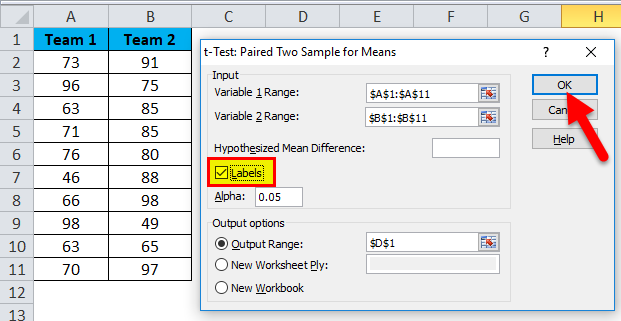
Step 7: From the D1 cell, it will start showing the test result.
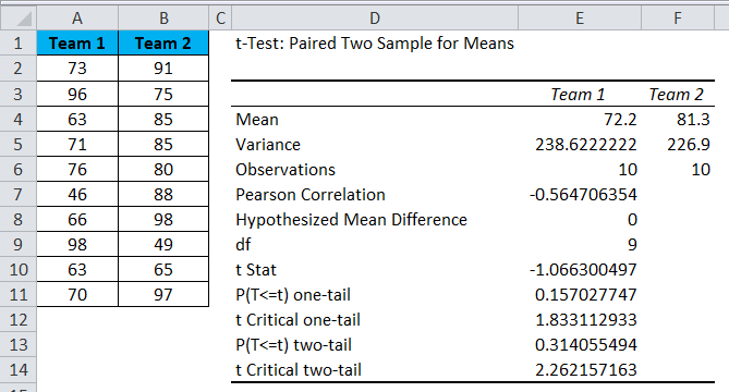
The result will show the mean value of two teams, Variance Value, how many observations are conducted or how many values taken into consideration, Pearson Correlation etc.…
If you P (T<=t) two-tail, it is 0.314, which is higher than the standard expected P-value of 0.05. This means data is not significant.
We can also do the T-test by using the built-in function T.TEST.
SOLVER Option – Example#2
A solver is nothing but solving the problem. SOLVER works like a goal seek in excel.
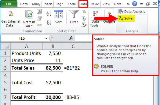
Look at the below image. I have data of product units, unit price, total cost, and the total profit.
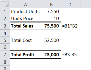
Units sold quantity is 7550 at a selling price of 10 per unit. The total cost is 52500, and the total profit is 23000.
As a proprietor, I want to earn a profit of 30000 by increasing the unit price. As of now, I don’t know how much units price I have to increase. SOLVER will help me to solve this problem.
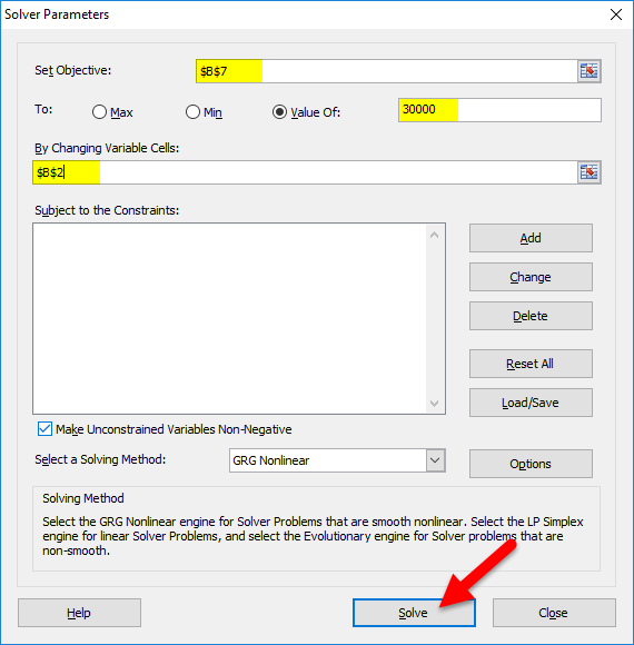
Step 1: Open SOLVER under the DATA tab.
Step 2: Set the objective cell as B7 and the value of 30000 and by changing the cell to B2. Since I don’t have any other special criteria to test, I am clicking on the SOLVE button.
Step 3: The Result will be as below:
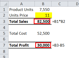
Ok, excel SOLVER solved the problem for me. To make a profit of 30000 I need to sell the products at 11 per unit instead of 10 per unit.
In this way, we can do the analyze the data.
Things to Remember
- We have many other analysis tests like Regression, F-test, ANOVA, Correlation, Descriptive techniques.
- We can add Excel Add-in as a data analysis tool pack.
- Analysis tool pack is available under VBA too.
Recommended Articles
This has been a guide to Data Analysis Tool in Excel. Here we discuss how to use the Excel Data Analysis Tool along with excel examples and a downloadable excel template. You may also look at these useful articles in excel –
- Pareto Analysis in Excel
- What-If Analysis in Excel
- Excel Regression Analysis
- Excel Quick Analysis