
Содержание
- Names in formulas
- Learn more about using names
- Define a name for a cell or cell range on a worksheet
- Manage names by using the Name Manager dialog box
- Need more help?
- How to Define and Edit a Named Range in Excel
- What to Know
- Defining and Managing Names with the Name Box
- Naming Rules and Restrictions
- What Is a Named Range?
- Defining and Managing Names with the Name Manager
- Deleting or Editing Names
- Filtering Names
- Defined Names and Scope in Excel
- Local Worksheet Level Scope
- Global Workbook Level Scope
- Scope Conflicts and Scope Precedence
Names in formulas
A name is a meaningful shorthand that makes it easier to understand the purpose of a cell reference, constant, formula, or table, each of which may be difficult to understand at first glance. The following information shows common examples of names and how they can improve clarity.
Example with no name
Example with a name
Learn more about using names
There are several types of names you can create and use.
Defined name A name representing a cell, range of cells, formula, or constant value. You can create your own defined name, or Excel can create a defined name for you, such as when you set a print area.
Table name A name for an Excel table, which is a collection of data about a particular subject stored in records (rows) and fields (columns). Excel creates a default Excel table name of Table1, Table2, and so on, each time you insert an Excel table. You can change a table’s name to make it more meaningful. For more information about Excel tables, see Using structured references with Excel tables.
All names have a scope, either to a specific worksheet (also called the local worksheet level) or to the entire workbook (also called the global workbook level). The scope of a name is the location within which the name is recognized without qualification. For example:
If you have defined a name, such as Budget_FY08, and its scope is Sheet1, that name, if not qualified, is recognized only in Sheet1, but not in other sheets.
To use a local worksheet name in another worksheet, you can qualify it by preceding it with the worksheet name. For example:
If you have defined a name, such as Sales_Dept_Goals, and its scope is the workbook, that name is recognized for all worksheets in that workbook, but not other workbooks.
A name must always be unique within its scope. Excel prevents you from defining a name that already exists within its scope. However, you can use the same name in different scopes. For example, you can define a name, such as GrossProfit, that is scoped to Sheet1, Sheet2, and Sheet3 in the same workbook. Although each name is the same, each name is unique within its scope. You might do this to ensure that a formula that uses the name, GrossProfit, is always referencing the same cells at the local worksheet level.
You can even define the same name, GrossProfit, for the global workbook level, but again the scope is unique. In this case, however, there can be a name conflict. To resolve this conflict, by default Excel uses the name defined for the worksheet because the local worksheet level takes precedence over the global workbook level. If you want to override the precedence and use the workbook name, you can disambiguate the name by prefixing the workbook name. For example:
You can override the local worksheet level for all worksheets in the workbook. One exception is for the first worksheet, which always uses the local name if there is a name conflict that cannot be overridden.
You define a name by using the:
Defined Names box on the formula bar This is best used for creating a workbook level name for a selected range.
Define name from selection You can conveniently create names from existing row and column labels by using a selection of cells in the worksheet.
New Name dialog box This is best used for when you want more flexibility in creating names, such as specifying a local worksheet level scope or creating a name comment.
Note: By default, names use absolute cell references.
You can enter a name by:
Typing Typing the name, for example, as an argument to a formula.
Using Formula AutoComplete Use the Formula AutoComplete drop-down list, where valid names are automatically listed for you.
Selecting from the Use in Formula command Select a defined name from a list available from the Use in Formula command in the Defined Names group on the Formulas tab.
You can also create a list of defined names in a workbook. Locate an area with two empty columns on the worksheet (the list will contain two columns, one for the name and one for a description of the name). Select a cell that will be the upper-left corner of the list. On the Formulas tab, in the Defined Names group, click Use in Formula, click Paste and then, in the Paste Names dialog box, click Paste List.
The following is a list of syntax rules for creating and editing names.
Valid characters The first character of a name must be a letter, an underscore character (_), or a backslash (). Remaining characters in the name can be letters, numbers, periods, and underscore characters.
Tip: You cannot use the uppercase and lowercase characters «C», «c», «R», or «r» as a defined name, because they are used as shorthand for selecting a row or column for the currently selected cell when you enter them in a Name or Go To text box.
Cell references disallowed Names cannot be the same as a cell reference, such as Z$100 or R1C1.
Spaces are not valid Spaces are not allowed as part of a name. Use the underscore character (_) and period (.) as word separators, such as, Sales_Tax or First.Quarter.
Name length A name can contain up to 255 characters.
Case sensitivity Names can contain uppercase and lowercase letters. Excel does not distinguish between uppercase and lowercase characters in names. For example, if you create the name Sales and then another name called SALES in the same workbook, Excel prompts you to choose a unique name.
Define a name for a cell or cell range on a worksheet
Select the cell, range of cells, or nonadjacent selections that you want to name.
Click the Name box at the left end of the formula bar.

Type the name you want to use to refer to your selection. Names can be up to 255 characters in length.
Note: You cannot name a cell while you are changing the contents of the cell.
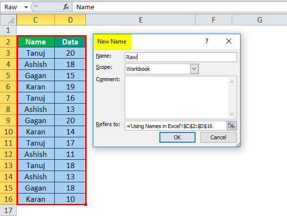
You can convert existing row and column labels to names.
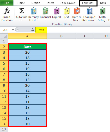
Select the range you want to name, including the row or column labels.
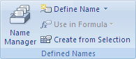
On the Formulas tab, in the Defined Names group, click Create from Selection.
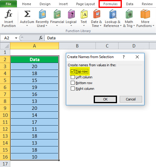
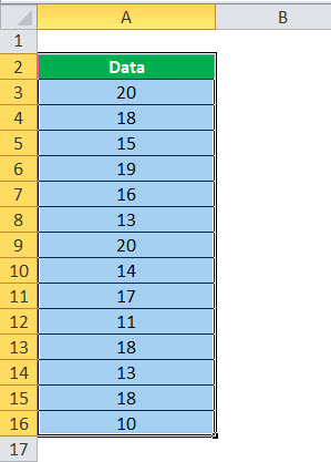
In the Create Names from Selection dialog box, designate the location that contains the labels by selecting the Top row, Left column, Bottom row, or Right column check box. A name created by using this procedure refers only to the cells that contain values and excludes the existing row and column labels.
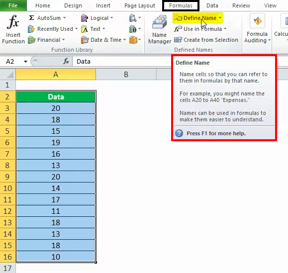
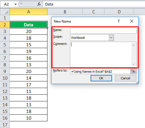
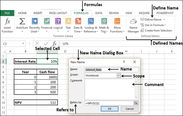
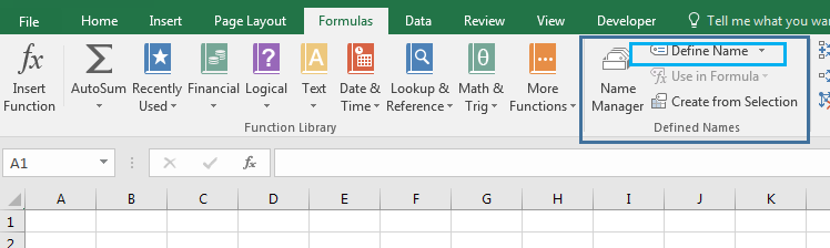
On the Formulas tab, in the Defined Names group, click Define Name.
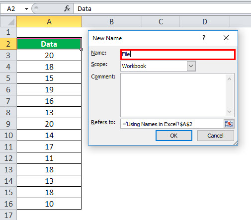
In the New Name dialog box, in the Name box, type the name you want to use for your reference.
Note: Names can be up to 255 characters in length.
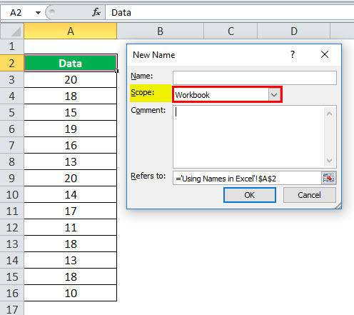
To specify the scope of the name, in the Scope drop-down list box, select Workbook or the name of a worksheet in the workbook.
Optionally, in the Comment box, enter a descriptive comment up to 255 characters.
In the Refers to box, do one of the following:
To enter a cell reference, type the cell reference.
Tip: The current selection is entered by default. To enter other cell references as an argument, click Collapse Dialog  (which temporarily shrinks the dialog box), select the cells on the worksheet, and then click Expand Dialog
  .
.
To enter a constant, type = (equal sign) and then type the constant value.
To enter a formula, type = and then type the formula.
To finish and return to the worksheet, click OK.
Tip: To make the New Name dialog box wider or longer, click and drag the grip handle at the bottom.
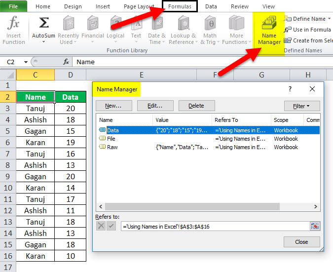
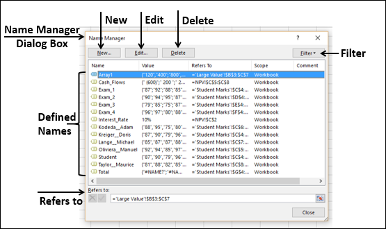
Manage names by using the Name Manager dialog box
Use the Name Manager dialog box to work with all the defined names and table names in a workbook. For example, you may want to find names with errors, confirm the value and reference of a name, view or edit descriptive comments, or determine the scope. You can also sort and filter the list of names, and easily add, change, or delete names from one location.
To open the Name Manager dialog box, on the Formulas tab, in the Defined Names group, click Name Manager.
The Name Manager dialog box displays the following information about each name in a list box:
One of the following:
A defined name, which is indicated by a defined name icon. 
A table name, which is indicated by a table name icon. 
The current value of the name, such as the results of a formula, a string constant, a cell range, an error, an array of values, or a placeholder if the formula cannot be evaluated. The following are representative examples:
«this is my string constant»
The current reference for the name. The following are representative examples:
A worksheet name, if the scope is the local worksheet level.
«Workbook,» if the scope is the global worksheet level.
Additional information about the name up to 255 characters. The following are representative examples:
This value will expire on May 2, 2007.
Don’t delete! Critical name!
Based on the ISO certification exam numbers.
You cannot use the Name Manager dialog box while you are changing the contents of a cell.
The Name Manager dialog box does not display names defined in Visual Basic for Applications (VBA), or hidden names (the Visible property of the name is set to «False»).
To automatically size the column to fit the longest value in that column, double-click the right side of the column header.
To sort the list of names in ascending or descending order, click the column header.
Use the commands in the Filter drop-down list to quickly display a subset of names. Selecting each command toggles the filter operation on or off, making it easy to combine or remove different filter operations to get the results you want.
To filter the list of names, do one or more of the following:
Names Scoped To Worksheet
Display only those names that are local to a worksheet.
Names Scoped To Workbook
Display only those names that are global to a workbook.
Names With Errors
Display only those names with values containing errors (such as #REF, #VALUE, or #NAME).
Names Without Errors
Display only those names with values that do not contain errors.
Display only names defined by you or by Excel, such as a print area.
Display only table names.
If you change a defined name or table name, all uses of that name in the workbook are also changed.
On the Formulas tab, in the Defined Names group, click Name Manager.
In the Name Manager dialog box, click the name that you want to change, and then click Edit.
Tip: You can also double-click the name.
In the Edit Name dialog box, in the Name box, type the new name for the reference.
In the Refers to box, change the reference, and then click OK.
In the Name Manager dialog box, in the Refers to box, change the cell, formula, or constant represented by the name.
To cancel unwanted or accidental changes, click Cancel  , or press ESC.
To save changes, click Commit  , or press ENTER.
The Close button only closes the Name Manager dialog box. It is not required for changes that have already been made.
On the Formulas tab, in the Defined Names group, click Name Manager.
In the Name Manager dialog box, click the name that you want to change.
Select one or more names by doing one of the following:
To select a name, click it.
To select more than one name in a contiguous group, click and drag the names, or press SHIFT and click the mouse button for each name in the group.
To select more than one name in a noncontiguous group, press CTRL and click the mouse button for each name in the group.
Click Delete. You can also press DELETE.
Click OK to confirm the deletion.
The Close button only closes the Name Manager dialog box. It is not required for changes that have already been made.
Need more help?
You can always ask an expert in the Excel Tech Community or get support in the Answers community.
Источник
How to Define and Edit a Named Range in Excel
Give descriptive names to specific cells or ranges of cells
What to Know
- Highlight the desired range of cells and type a name in the Name Box above column A in the worksheet.
- Alternatively, highlight the desired range, select the Formulas tab on the ribbon, then select Define Name.
- To manage range names, go to the Formulas tab, select Name Manager, choose a name, then select Delete or Edit.
This article explains how to define and edit names for ranges in Excel for Microsoft 365, Excel 2019, 2016, 2013, and 2010.
Defining and Managing Names with the Name Box
One way, and possibly the easiest way, of defining names is using the Name Box, located above column A in the worksheet. You can use this method to create unique names that are recognized by every sheet in a workbook.
:max_bytes(150000):strip_icc()/NameBox-5be366ed46e0fb00519ef15a.jpg)
To create a name using the Name Box as shown in the image above:
Highlight the desired range of cells in the worksheet.
:max_bytes(150000):strip_icc()/Capture-727a8d317fe2483e9c44cd3e2c537c31.JPG)
Type the desired name for that range in the Name Box, such as Jan_Sales.
:max_bytes(150000):strip_icc()/Capture-7831254244634c2b933286216bca3dc7.JPG)
Press the Enter key on the keyboard. The name is displayed in the Name Box.
The name is also displayed in the Name box whenever the same range of cells is highlighted in the worksheet. It is also displayed in the Name Manager.
Naming Rules and Restrictions
Syntax rules to remember when creating or editing names for ranges are as follows:
- A name can’t contain spaces.
- The first character of a name must be either a letter, underscore, or backslash.
- The remaining characters can only be letters, numbers, periods, or underscore characters.
- The maximum name length is 255 characters.
- Uppercase and lowercase letters are indistinguishable to Excel, so Jan_Sales and jan_sales are seen as the same name by Excel.
- Cell reference cannot be used as names such as A25 or R1C4.
What Is a Named Range?
A named range, range name, or defined name all refer to the same object in Excel; it’s a descriptive name — such as Jan_Sales or June_Precip — that is attached to a specific cell or range of cells in a worksheet or workbook. Named ranges make it easier to use and identify data when creating charts, and in formulas such as:
Additionally, since a named range does not change when a formula is copied to other cells, it provides an alternative to using absolute cell references in formulas. There are three methods for defining a name in Excel: using the name box, the new name dialog box, or the name manager.
Defining and Managing Names with the Name Manager
A second method for defining names is to use the New Name dialog box. This dialog box is opened using the Define Name option located in the middle of the Formulas tab of the ribbon. The New Name dialog box makes it easy to define names with a worksheet level scope.
:max_bytes(150000):strip_icc()/NamedRangeNameManager-5c192805c9e77c0001a4b91c.jpg)
To create a name using New Name dialog box:
Highlight the desired range of cells in the worksheet.
Select the Formulas tab of the ribbon.
:max_bytes(150000):strip_icc()/Capture-11ec717ce0af4707abb8369846d3ec75.JPG)
Select the Define Name option to open the New Name dialog box.
:max_bytes(150000):strip_icc()/Capture-04aecfcf1d65477698be827ac64a6769.JPG)
Enter the Name, Scope, and Range in the dialog box.
:max_bytes(150000):strip_icc()/Capture-6bed281edf3e4ae996fd851616667b19.JPG)
Once completed, select OK to return to the worksheet. The name displays in the Name Box whenever the defined range is selected.
:max_bytes(150000):strip_icc()/Capture-e6dfab231cdc4cbc97f73322574818ae.JPG)
The Name Manager can be used to both define and manage existing names; it is located next to the Define Name option on the Formulas tab of the ribbon.
When defining a name in the Name Manager it opens the New Name dialog box outlined above. The complete list of steps are as follows:
Select the Formulas tab of the ribbon.
Select the Name Manager icon in the middle of the ribbon to open the Name Manager.
:max_bytes(150000):strip_icc()/Capture-827f3256441a4485b4bcf92d8cf4e598.JPG)
In the Name Manager, select the New button to open the New Name dialog box.
:max_bytes(150000):strip_icc()/Capture-4831609966814ee191907d9cbad2c061.JPG)
Enter a Name, Scope, and Range. Select OK to return to the worksheet. The name displays in the Name Box whenever the defined range is selected.
Deleting or Editing Names
With the Name Manager open:
In the window containing the list of names, select the name to be deleted or edited.
:max_bytes(150000):strip_icc()/Capture-8f010c67f6134e50b41eebf73eca2b44.JPG)
To delete the name, select the Delete button above the list window.
:max_bytes(150000):strip_icc()/Capture-022c5ce7266b48e39b97f10e31c46423.JPG)
To edit the name, select the Edit button to open the Edit Name dialog box.
In the Edit Name dialog box, you can edit the chosen name, add comments about the name, or change the existing range reference.
:max_bytes(150000):strip_icc()/Capture-d793543ee3f54ff0836dffe6ebe99f6c.JPG)
The scope of an existing name cannot be changed using the edit options. To change the scope, delete the name and redefine it with the correct scope.
Filtering Names
The Filter button in the Name Manager makes it easy to:
- Find names with errors – such as an invalid range.
- Determine the scope of a name – whether worksheet level or workbook.
- Sort and filter listed names – defined (range) names or table names.
The filtered list is displayed in the list window in the Name Manager.
Defined Names and Scope in Excel
All names have a scope which refers to the locations where a specific name is recognized by Excel. A name’s scope can be for either individual worksheets (local scope) or for an entire workbook (global scope). A name must be unique within its scope, but the same name can be used in different scopes.
The default scope for new names is the global workbook level. Once defined, the scope of a name cannot easily be changed. To change the scope of a name, delete the name in the Name Manager and redefine it with the correct scope.
Local Worksheet Level Scope
A name with a worksheet level scope is valid only for the worksheet for which it was defined. If the name Total_Sales has a scope of sheet 1 of a workbook, Excel will not recognize the name on sheet 2, sheet 3, or any other sheet in the workbook. This makes it possible to define the same name for use on multiple worksheets – as long as the scope for each name is restricted to its particular worksheet.
Using the same name for different sheets might be done to ensure continuity between worksheets and ensure that formulas that use the name Total_Sales always refer to the same range of cells in multiple worksheets within a single workbook.
To distinguish between identical names with different scopes in formulas, precede the name with the worksheet name, such as:
Names created using the Name Box always have a global workbook level scope unless both sheet name and the range name are entered into the name box when the name is defined.
:max_bytes(150000):strip_icc()/Sheets-5bf079d246e0fb0051860dee.jpg)
Examples:
- Name: Jan_Sales, Scope — global workbook level
- Name: Sheet1!Jan_Sales, Scope — local worksheet level
Global Workbook Level Scope
A name defined with a workbook level scope is recognized for all worksheets in that workbook. A workbook level name can, therefore, only be used once within a workbook, unlike the sheet level names discussed above.
A workbook level scope name is not, however, recognized by any other workbook, so global level names can be repeated in different Excel files. For example, if the Jan_Sales name has a global scope, the same name could be used in different workbooks titled 2012_Revenue, 2013_Revenue, and 2014_Revenue.
Scope Conflicts and Scope Precedence
It is possible to use the same name at both the local sheet level and workbook level because the scope for the two would be different. Such a situation, however, would create a conflict whenever the name was used.
To resolve such conflicts, in Excel, names defined for the local worksheet level take precedence over the global workbook level. In such a situation, a sheet-level name of 2014_Revenue would be used instead of a workbook level name of 2014_Revenue.
To override the rule of precedence, use the workbook level name in conjunction with a specific sheet-level name such as:
The one exception to overriding precedence is a local worksheet level name that has a scope of sheet 1 of a workbook. Scopes linked to sheet 1 of any workbook cannot be overridden by global level names.
Источник
What is Name Range in Excel?
The name range in Excel is the range that has been given a name for future reference. To make a range as a named range, select the range of data and then insert a table. Then, we put a name to the range from the Name Box on the left-hand side of the window. After this, we can refer to the range by its name in any formula.
The name range in Excel makes it much cooler to keep track of things, especially when using formulas. You can assign a name to a range. No problem with any change in that range; you need to update the range from the Name Manager in ExcelThe name manager in Excel is used to create, edit, and delete named ranges. For example, we sometimes use names instead of giving cell references. By using the name manager, we can create a new reference, edit it, or delete it.read more. You do not need to update every formula manually. Similarly, you can create a name for a formula. Then, if you want to use that formula in another formula or another location, refer to it by name.
- The name ranges are significant because you can put any names in your formulas without considering cell references/addresses. Furthermore, you can assign the range with any name.
- Create a named range for any data or a named constant and use these names in your formulas in place of data references. In this way, you can make your formulas easier to comprehend better. A named range is just a human-understandable name for a range of cells in Excel.
- Using the name range in Excel, you can simplify and comprehend your formulas better. For example, you can assign a name for a range in an excel sheet for a function, a constant, or table data. Once you start using the names in your Excel sheet, you can easily understand these names.
Table of contents
- What is Name Range in Excel?
- Define Names For a Selected Range
- Excel names the cells based on the labels in the range you designated.
- Update named ranges in the Name Manager (Control + F3)
- How to Use Name Range in Excel?
- Example #1 Create a name by using the Define Name option
- Example #2 Make a named range by using Excel Name Manager
- Name Range using VBA.
- Things to Remember
- Recommended Articles
- Define Names For a Selected Range
Define Names For a Selected Range
- Select the data range you want to assign a name, then select formulas and create from the selection.
- Click on the “Create Names from Selection,” then select the “Top row,” “Left column,” “Bottom row,” or “Right column” checkbox and select “OK.”
Excel names the cells based on the labels in the range you designated.
- Use names in formulas, then select a cell and enter a formula.
- Place the cursor where you want to use the name range formula.
- Type the first letter of the name, and select the name from the list that appears.
- Or, select “Formulas,” then use in formula and select the name you want to use.
- Press the “Enter” key.
Update named ranges in the Name Manager (Control + F3)
You can update the name from the Name Manager. Press “Ctrl” and “F3” to update the name. Select the name you want to change, then change the reference range directly.
How to Use Name Range in Excel?
Let us understand the working of conditional formatting by simple Excel examples.
You can download this Using Names in Excel Template here – Using Names in Excel Template
Example #1 Create a name by using the Define Name option
Below are the steps to create a name by using the “Define Name” option:
- First, select the cell(s).

- On the “Formulas” tab, click the “Define Name” in the “Defined Names” group.

- In the “New Name” dialog box, specify three things:

- First, in the “Name” box, type the range name.

- In the “Scope” drop-down, set the name scope (Workbook by default).

- In the “Refers to” box, check the reference and correct it if needed. Finally, click “OK” to save the changes and close the dialog box.


Example #2 Make a named range by using Excel Name Manager
- Go to the “Formulas” tab, then the “Defined Names” group, and click the “Name Manager” or press “Ctrl + F3” (the preferred way).
- In the top left-hand corner of the “Name Manager” dialog window, click the “New… button:”
Name Range using VBA.
We can apply the naming in VBA; here is the example as follows:
Sub sbNameRange()
‘Adding a Name
Names.Add Name:=”myData”, RefersTo:=”=Sheet1!$A$1:$A$10″
‘OR
‘You can use Name property of a Range.
Sheet1.Range(“$A$1:$A$10”).Name = “myData”
End Sub
Things to Remember
We must follow the below instruction while using the name range.
- The names can start with a letter, backslash (), or an underscore (_).
- The name should be under 255 characters long.
- The names must be continuous and cannot contain spaces and most punctuation characters.
- There must be no conflict with cell references in names using in excelCell reference in excel is referring the other cells to a cell to use its values or properties. For instance, if we have data in cell A2 and want to use that in cell A1, use =A2 in cell A1, and this will copy the A2 value in A1.read more.
- We can use single letters as names, but the letters “r” and “c” are reserved in Excel.
- The names are not case-sensitive – “Tanuj”, “TANUJ”, and “TaNuJ” are all the same in Excel.
Recommended Articles
This article is a guide to the Name Range in Excel. We discuss using names in Excel, practical examples, and downloadable Excel templates here. You also may look at these useful functions in Excel: –
- VBA RangeRange is a property in VBA that helps specify a particular cell, a range of cells, a row, a column, or a three-dimensional range. In the context of the Excel worksheet, the VBA range object includes a single cell or multiple cells spread across various rows and columns.read more
- Data Tables ExcelA data table in excel is a type of what-if analysis tool that allows you to compare variables and see how they impact the result and overall data. It can be found under the data tab in the what-if analysis section.read more
- Data Validation using ExcelThe data validation in excel helps control the kind of input entered by a user in the worksheet.read more
- Paste SpecialPaste special in Excel allows you to paste partial aspects of the data copied. There are several ways to paste special in Excel, including right-clicking on the target cell and selecting paste special, or using a shortcut such as CTRL+ALT+V or ALT+E+S.read more
Although cell numbers are at the foundation of everything Excel does, it’s much easier to remember names, such as Item Number and Quantity, than it is to remember cell numbers, such as A1:A100. Excel makes this easy.
Address Data by Name
Excel uses the same technique for defining named cells and named ranges: the Name box at the left end of the Formula bar. To name a cell, select it, type the name you want into the Name box, as shown in Figure 3-1, and press Enter. To name a range of cells, select the range, type the name you want for that range in the Name box, and press Enter.
Figure 3-1. Naming a cell MyFavoriteCell
The drop-down list at the right side of the Name box enables you to find your named ranges and cells again. (See [Example #44] at the end of this tutorial for more ways to locate ranges.) If you happen to select a range precisely, its name will appear in the Name box instead of the usual cell references.
In formulas, you can use these names in place of cell identifiers or ranges. If you name cell E4 «date,» for instance, you could write =date instead of =E4. Similarly, if you create a range called «quantity» in A3:A10 and want a total of the values in it, your formula could say =SUM(quantity) rather than =SUM(A3:A10).
As spreadsheets grow larger and more intricate, named cells and ranges are crucial tools for keeping them manageable.
- Use the Same Name for Ranges on Different Worksheets
- Create Custom Functions Using Names
- Create Ranges That Expand and Contract
- Nest Dynamic Ranges for Maximum Flexibility
- Identify Named Ranges on a Worksheet
by updated Aug 01, 2016
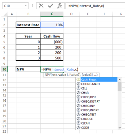
While doing Data Analysis, referring to various data will be more meaningful and easy if the reference is by Names rather than cell references – either a single cell or a range of cells. For example, if you are calculating Net Present Value based on a Discount Rate and a series of Cash Flows, the formula
Net_Present_Value = NPV (Discount_Rate, Cash_Flows)
is more meaningful than
C10 = NPV (C2, C6:C8)
With Excel, you can create and use meaningful names to various parts of your data. The advantages of using range names include −
-
A meaningful Range name (such as Cash_Flows) is much easier to remember than a Range address (such as C6:C8).
-
Entering a name is less error prone than entering a cell or range address.
-
If you type a name incorrectly in a formula, Excel will display a #NAME? error.
-
You can quickly move to areas of your worksheet by using the defined names.
-
With Names, your formulas will be more understandable and easier to use. For example, a formula Net_Income = Gross_Income – Deductions is more intuitive than C40 = C20 – B18.
-
Creating formulas with range names is easier than with cell or range addresses. You can copy a cell or range name into a formula by using formula Autocomplete.
In this chapter, you will learn −
- Syntax rules for names.
- Creating names for cell references.
- Creating names for constants.
- Managing the names.
- Scope of your defined names.
- Editing names.
- Filtering names.
- Deleting names.
- Applying names.
- Using names in a formula.
- Viewing names in a workbook.
- Using paste names and paste list.
- Using names for range intersections.
- Copying formulas with names.
Copying Name using Formula Autocomplete
Type the first letter of the name in the formula. A drop-down box appears with function names and range names. Select the required name. It is copied into your formula.
Range Name Syntax Rules
Excel has the following syntax rules for names −
-
You can use any combination of letters, numbers and the symbols — underscores, backslashes, and periods. Other symbols are not allowed.
-
A name can begin with a character, underscore or backslash.
-
A name cannot begin with a number (example — 1stQuarter) or resemble a cell address (example — QTR1).
-
If you prefer to use such names, precede the name with an underscore or a backslash (example — 1stQuarter, _QTR1).
-
Names cannot contain spaces. If you want to distinguish two words in a name, you can use underscore (example- Cash_Flows instead of Cash Flows)
-
Your defined names should not clash with Excel’s internally defined names, such as Print_Area, Print_Titles, Consolidate_Area, and Sheet_Title. If you define the same names, they will override the Excel’s internal names and you will not get any error message. However, it is advised not to do so.
-
Keep the names short but understandable, though you can use up to 255 characters
Creating Range Names
You can create Range Names in two ways −
-
Using the Name box.
-
Using the New Name dialog box.
-
Using the Selection dialog box.
Create a Range Name using the Name Box
To create a Range name, using the Name box that is to the left of formula bar is the fastest way. Follow the steps given below −
Step 1 − Select the range for which you want to define a Name.
Step 2 − Click on the Name box.
Step 3 − Type the name and press Enter to create the Name.
Create a Range Name using the New Name dialog box
You can also create Range Names using the New Name dialog box from Formulas tab.
Step 1 − Select the range for which you want to define a name.
Step 2 − Click the Formulas tab.
Step 3 − Click Define Name in the Defined Names group. The New Name dialog box appears.
Step 4 − Type the name in the box next to Name
Step 5 − Check that the range that is selected and displayed in the Refers box is correct. Click OK.
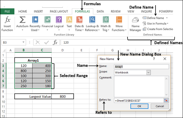
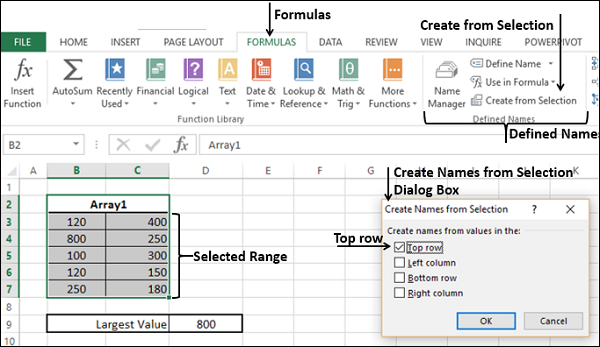
Create a Range Name using the Create Names from Selection dialog box
You can also create Range names using the Create Names from the Selection dialog box from Formulas tab, when you have Text values that are adjacent to your range.
Step 1 − Select the range for which you want to define a name along with the row / column that contains the name.
Step 2 − Click the Formulas tab.
Step 3 − Click Create from Selection in the Defined Names group. The Create Names from Selection dialog box appears.
Step 4 − Select top row as the Text appears in the top row of the selection.
Step 5 − Check the range that got selected and displayed in the box next to Refers to be correct. Click OK.
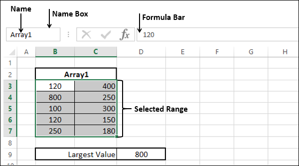
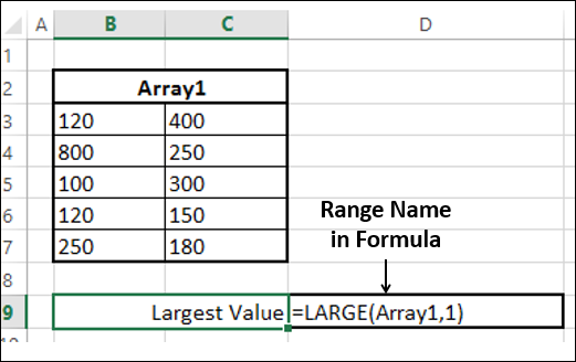
Now, you can find the largest value in the range with =Sum(Student Name), as shown below −
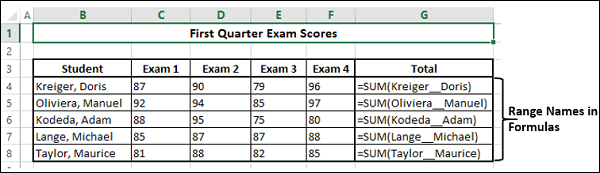
You can create names with multiple selection also. In the example given below, you can name the row of marks of each student with the student’s name.
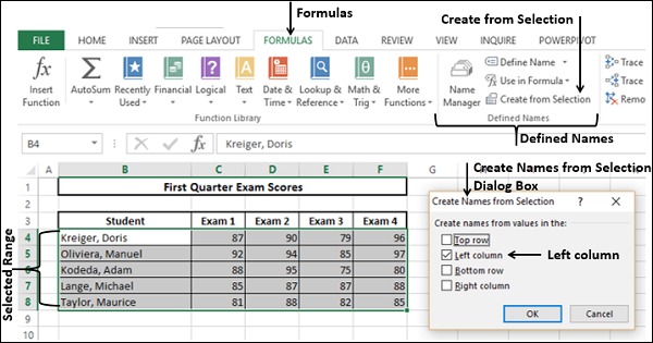
Now, you can find the total marks for each student with =Sum (student name), as shown
below.
Creating Names for Constants
Suppose you have a constant that will be used throughout your workbook. You can assign a name to it directly, without placing it in a cell.
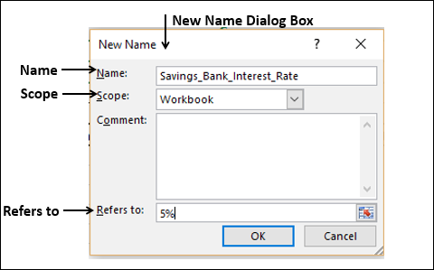
In the example below, Savings Bank Interest Rate is set to 5%.
- Click Define Name.
- In the New Name dialog box, type Savings_Bank_Interest_Rate in the Name box.
- In Scope, select Workbook.
- In Refers to box, clear the contents and type 5%.
- Click OK.
The Name Savings_Bank_Interest_Rate is set to a constant 5%. You can verify this in Name Manager. You can see that the value is set to 0.05 and in the Refers to =0.05 is placed.
Managing Names
An Excel Workbook can have any number of named cells and ranges. You can manage these names with the Name Manager.
-
Click the Formulas tab.
-
Click Name Manager in the Defined Names group. The Name Manager dialog box appears. All the names defined in the current workbook are displayed.
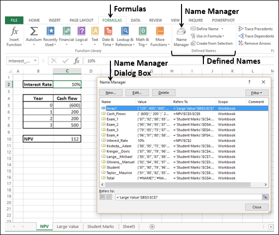
The List of Names are displayed with the defined Values, Cell Reference (including Sheet Name), Scope and Comment.
The Name Manager has the options to −
-
Define a New Name with the New Button.
-
Edit a Defined Name.
-
Delete a Defined Name.
-
Filter the Defined Names by Category.
-
Modify the Range of a Defined Name that it Refers to.
Scope of a Name
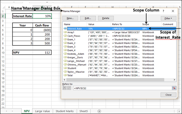
The Scope of a name by default is the workbook. You can find the Scope of a defined names from the list of names under the Scope column in the Name Manager.
You can define the Scope of a New Name when you define the name using New Name dialog box. For example, you are defining the name Interest_Rate. Then you can see that the Scope of the New Name Interest_Rate is the Workbook.
Suppose you want the Scope of this interest rate restricted to this Worksheet only.
Step 1 − Click the down-arrow in the Scope Box. The available Scope options appear in the drop-down list.
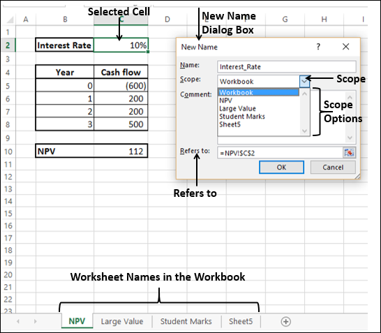
The Scope options include Workbook, and the sheet names in the workbook.
Step 2 − Click the current worksheet name, in this case NPV and click OK. You can define / find the sheet name in the worksheet tab.
Step 3 − To verify that Scope is worksheet, click Name Manager. In the Scope column, you will find NPV for Interest_Rate. This means you can use the Name Interest_Rate only in the
Worksheet NPV, but not in the other Worksheets.
Note − Once you define the Scope of a Name, it cannot be modified later.
Deleting Names with Error Values
Sometimes, it may so happen that Name definition may have errors for various reasons. You can delete such names as follows −
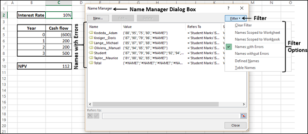
Step 1 − Click Filter in the Name Manager dialog box.
The following filtering options appear −
- Clear Filter
- Names Scoped to Worksheet
- Names Scoped to Workbook
- Names with Errors
- Names without Errors
- Defined Names
- Table Names
You can apply Filter to the defined Names by selecting one or more of these options.
Step 2 − Select Names with Errors. Names that contain error values will be displayed.
Step 3 − From the obtained list of Names, select the ones you want to delete and click Delete.
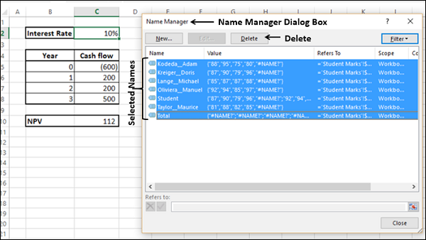
You will get a message, confirming delete. Click OK.
Editing Names
You can use the Edit option in the Name Manager dialog box to −
-
Change the Name.
-
Modify the Refers to range
-
Edit the Comment in a Name.
Change the Name
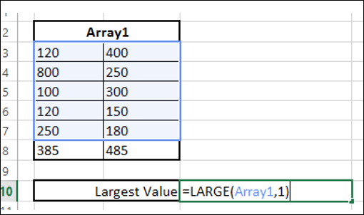
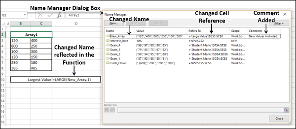
Step 1 − Click the cell containing the function Large.
You can see, two more values are added in the array, but are not included in the function as they are not part of Array1.
Step 2 − Click the Name you want to edit in the Name Manager dialog box. In this case, Array1.
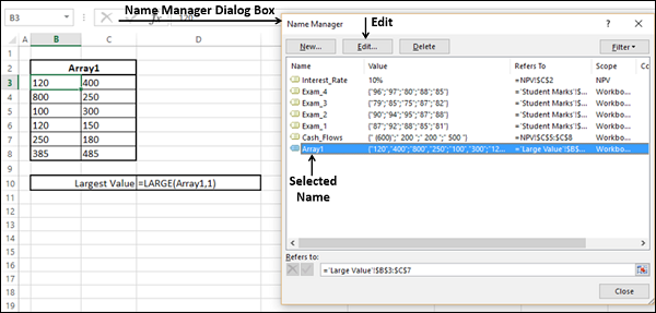
Step 3 − Click Edit. The Edit Name dialog box appears.
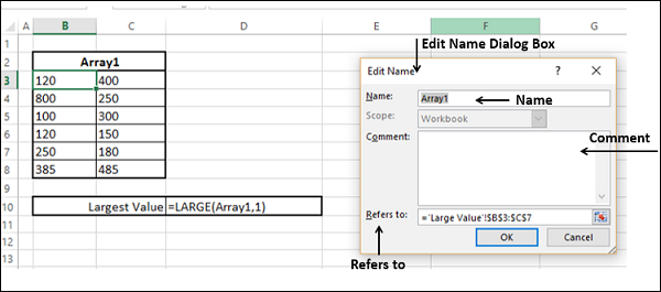
Step 4 − Change the Name by typing the new name that you want in the Name Box.
Step 5 − Click the Range button to the right of Refers to Box and include the new cell references.
Step 6 − Add a Comment (Optional)
Notice that Scope is deactive and hence cannot be changed.
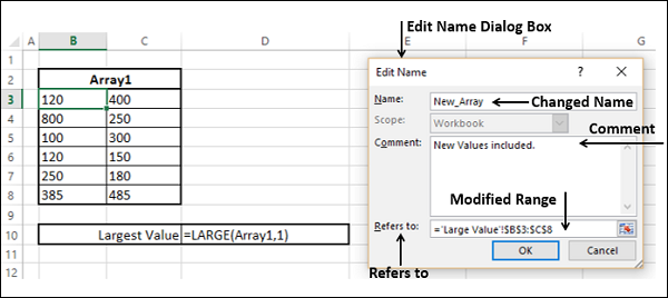
Click OK. You will observe the changes made.
Applying Names
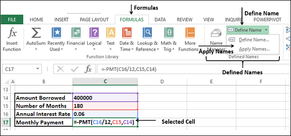
Consider the following example −
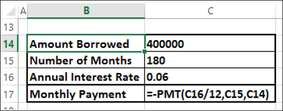
As you observe, names are not defined and used in PMT function. If you place this function somewhere else in the worksheet, you also need to remember where exactly the parameter values are. You know that using names is a better option.
In this case, the function is already defined with cell references that do not have names. You can still define names and apply them.
Step 1 − Using Create from Selection, define the names.
Step 2 − Select the cell containing the formula. Click  next to Define Name in the Defined Names group on the Formulas tab. From the drop-down list, click Apply Names.
Step 3 − The Apply Names dialog box appears. Select the Names that you want to Apply and click OK.
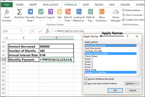
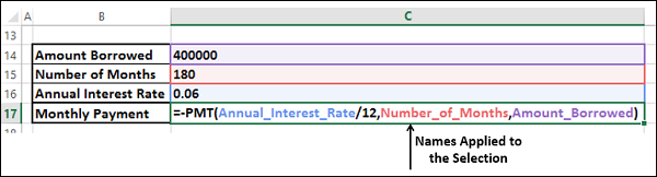
The selected names will be applied to the selected cells.
You can also Apply Names to an entire worksheet, by selecting the worksheet and repeating the above steps.
Using Names in a Formula
You can use a Name in a Formula in the following ways −
-
Typing the Name if you remember it, or
-
Typing first one or two letters and using the Excel Formula Autocomplete feature.
-
Clicking Use in Formula in the Defined Names group on the Formulas tab.
-
Select the required Name from the drop-down list of defined names.
-
Double-click on that name.
-
-
Using the Paste Name dialog box.
-
Select the Paste Names option from the drop-down list of defined names. The
Paste Name dialog box appears. -
Select the Name in the Paste Names dialog box and double-click it.
-
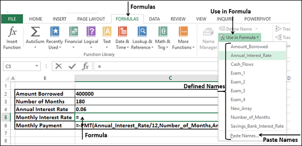
Viewing Names in a Workbook
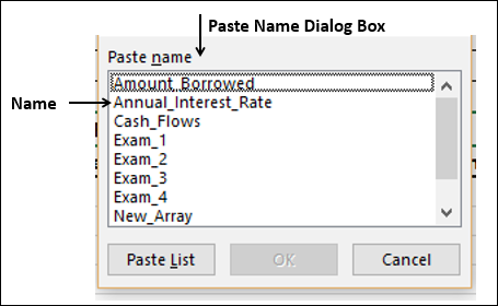
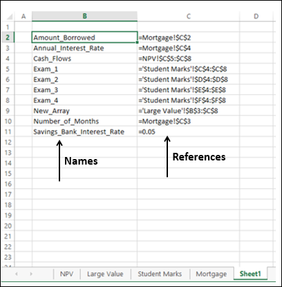
You can get all the Names in your workbook along with their References and Save them or Print them.
-
Click an empty Cell where you want to copy the Names in your workbook.
-
Click Use in Formula in the Defined Names group.
-
Click Paste Names from the drop-down list.
-
Click Paste List in the Paste Name dialog box that appears.

The list of names and their corresponding references are copied at the specified location on your worksheet as shown in the screen shot given below −
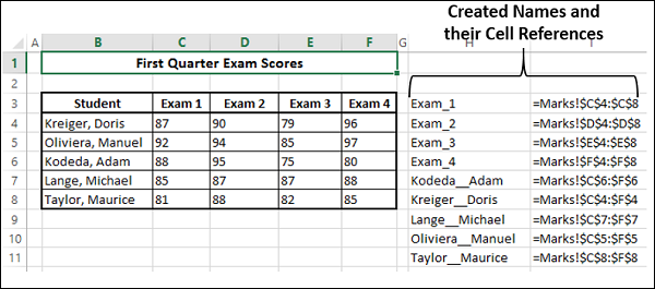
Using Names for Range Intersections
Range Intersections are those individual cells that have two Ranges in common.
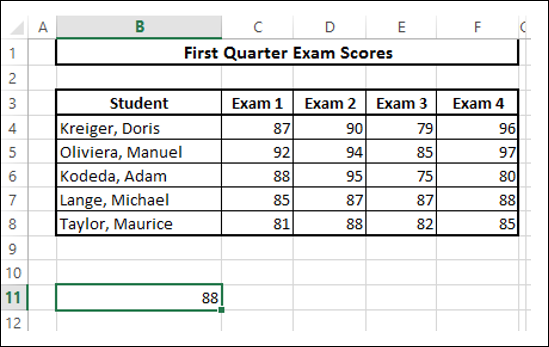
For example, in the data given below, the Range B6:F6 and the Range C3:C8 have Cell C6 in common, which actually represents the marks scored by the student Kodeda, Adam in Exam 1.
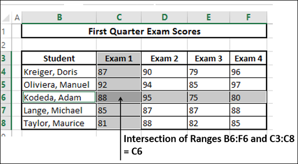
You can make this more meaningful with the Range Names.
-
Create Names with Create from Selection for both Students and Exams.
-
Your Names will look as follows −
-
Type =Kodeda_Adam Exam_1 in B11.
Here, you are using the Range Intersection operation, space between the two ranges.
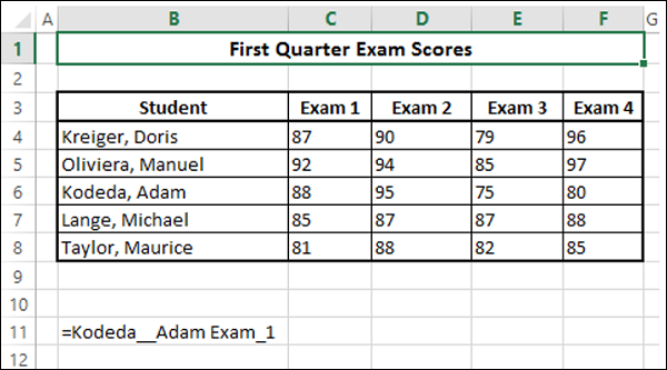
This will display marks of Kodeda, Adam in Exam 1, that are given in Cell C6.
Copying Formulas with Names
You can copy a formula with names by Copyand Paste within the same worksheet.
You can also copy a formula with names to a different worksheet by copy and paste, provided all the names in the formula have workbook as Scope. Otherwise, you will get a #VALUE error.
In this article, we will learn How to use Names in a Formula in Excel.
Scenario :
While working on Excel, you’ve must have heard about named ranges in excel. Maybe from a friend, colleague or some online tutorial. I have mentioned it many times in my articles. In this article we will learn about Named Range in Excel and will explore each and every aspect of it.
Named Ranges in Excel
Formulas -> Name Manager -> Define Name
Well, named ranges are nothing but some excel ranges that are given some meaningful name. For example if you have a cell say B1, containing everyday targets, you can name that cell as specifically “Target”. Now you can use “Target” to refer at A1 instead of writing B1.
In a nutshell, Named range is just naming of ranges.
How to name a range in Excel?
Define name manually:
To define a name to a range you can use shortcut CTRL + F3. Or you can follow these steps.
Now you can refer to it by just typing its name.
There are some rules to follow while creating names. Here are some.
- Names should not start from digits or special characters other than underscore (_) and backslash().
- Names can’t have spaces and any special characters except _ and .
- Range should not be named as cell references. For example A1, B1 or AZ100 etc.
- You can’t name a range as “r” and “c” because they are reserved for row and columns references.
- Two named ranges can’t have the same name in a workbook.
- Same range can have multiple names.
Well most of the time you will be working with structured data tables. They will have column and rows with column headings and row headings. And most of the time these names are meaningful to the data and you’d like to name your range as these column headings. Excel provides a tool to automatically name ranges using headings. Follow these steps.
Now each column is named as their heading. Whenever you type a formula, these names will be listed as options which can be accessed.
When we tablise a data in excel using CTRL + T, the column heading automatically is assigned as the name of the respective column. You should explore Excel Tables and their benefits.
Well there will be times when you would like to see all available named ranges in the workbook. To see all name ranges Press CTRL+F3. Or you can go to Formula Tab > Name Manager. This will list all named ranges that are available on the workbook. You can Edit available named ranges, delete them, add new names.
One Range Multiple Names
Excel allows users to name the same range with different names. For example range A2:A10 can be named ‘Customers’ and ‘Clients’ both at same time. Both names will refer to the same range A2:A10.
But you can’t have the same names for two different ranges. This is good. This eliminates the chance of ambiguity.
Get List of Named Ranges on Sheet
So if you want to have a list of named ranges and the ranges they are covering you can use this shortcut for pasting them in place in a sheet.
- Select a cell where you want to get a list of named ranges.
- Press F3. This will open a paste list dialogue box.
- Click on the paste list button.

- The list will be pasted on selected cells and onwards.


If you double click on the named ranges name in the paste name box, they will get written as formulas in the cell. Try it.
Update Named Ranges Manually
Well when you insert a cell inside a named range it updates automatically and expands it. But if you add data at the end of the table, you’ll need to update the named range. To update Named Ranges follow these steps.
- Press CTRL+F3 to open the name manager.
- Click on the named range that you want to edit. Click on Edit.
- In Refers to column type the range to which you want to expand and hit OK.
And It’s done. This is manual updating of named ranges. However, we can make it dynamic by using some formulas.
Update Named Ranges Dynamically
It is wise to make your named ranges dynamic so that you don’t have to edit them whenever your data overflows the predefined range.
I have covered it in a separate article called Dynamic Named ranges. You can learn and understand the benefits of it in detail here.
Deleting Named Ranges
When you delete the sum part of the named range, it auto adjusts its range. But when you delete the whole name range vanishes from the name list. Any formula, dependent on those ranges will show #REF error or they will give incorrect output (counting functions).
For any reason, if you want to delete named ranges, just follow these steps.
- Press CTRL+F3. Name manager will open.
- Select Named Ranges that you want to delete.
- Click on the Delete button or hit Delete button on keyboard.

Caution: Before you delete the named ranges make sure that no formulas are dependent on these names. If there is any, convert them to ranges first. Otherwise you’ll see #REF error.
Deleting Names with Errors
Excel provides tools to delete names that have errors only. You don’t need to identify each of them by yourself. To delete names with errors, follow these steps:
- Open Name Manager (CTRL+F3).
- Click on Filter drop down on right- upper corner.
- Select “Name with Errors”

- Select All and hit the delete button.

And they are gone. All the names with errors will be deleted from record immediately.
Named Ranges With Formulas
Best use of named ranges are explored with formulas. The Formulas get really flexible and readable with Named ranges. Let’s see how.
Easy To Write Formulas
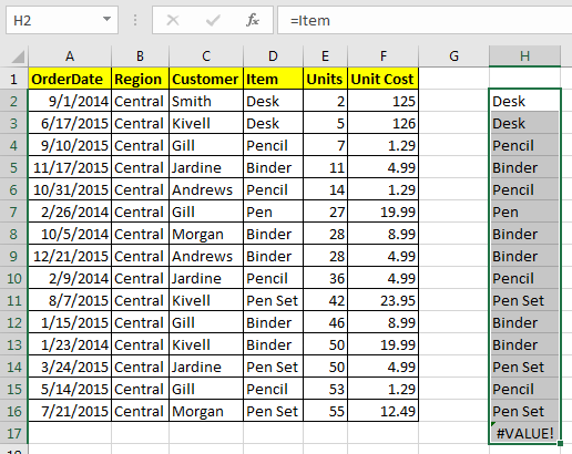
Now let’s say you have named a range as “Items”. Now the Items list you want to count “Pencils”. With names it is easy to write this COUNTIF formula. Just write
=COUNTIF(Item,»Pencil»)
As soon as you write the opening parenthesis of formula the list of available named ranges will appear
Without name you would write a give a range to COUNTIF function of Excel, for which you may have to look at the range first then select the range or type it in formula.
Excel Serves the Available Name Ranges.
The named ranges are shown as suggestions when you type any letter. As excel shows the list of formulas. For example if you type =u, each formula and named range will be displayed starting with u, so that you can use them easily.

Make Constants using Named Ranges
So far, we learned about naming ranges but you can actually name values too. For example if your client name is Sunder Pichai then you can make a name “Client” and it refers to write “Sundar Pichai”. Now whenever you will write =Client in any cell it will show Sundar Pichai.


Not only text, but you can also assign numbers as constant to work with. For example, you define a target. Or the value of something that will not change.
Absolute and Relative Referencing with Named Ranges
The referencing with Named ranges in is very flexible. For example if you write the name of a named range in a relative cell to the named range, it will behave like a relative reference. See below image.
But when you use it with formulas it will behave as absolute. Well most of the time you’ll be using them with formulas, so you can say that they are by default Absolute but actually they are flexible.

But we can make them relative too.
How to make Relative Named Ranges in Excel?
Let’s say if i want to name a range “Befor” which will refer to cell left to wherever it is written. How do I do that? Follow these steps:
- Press CTRL+F3
- Click on New
- Type “Befor” in the ‘Name’ Section.
- In ‘Refers to:’ section write address of cell in left. For example if you are in cell B1 then write “=A2” in ‘Refers to:’ section. Make sure that it does not have a $ sign.

Now wherever you will write the “Befor” in formula, it will refer to cell left to it.

Here, I used it before in the COLUMN function. The formula returns the column number of the left cell where it is written. To my suprise, A1 shows the column number of the last column. Which means the sheet is circulare. I thought it will show an #REF error.
Give Name to Often Used Formulas?
Now this one is amazing. Many times you use the same formula again and again in a worksheet. For example you may want to check if a name is in your customer list or not. And this need may occur many times. For this you’ll write same complex formula every time.
=IF(COUNTIF(Customer,I3),»In List»,»Not in List»)
How about, if you just type ‘=IsInCustomer’ in a cell and it will show you if the value in the left cell is in the customer list or not?

For example, I have prepared a table here. Now i just want to type “=IsInCustomer” in J5 and i would like to see if the value in I5 is in the Customer list or Not. To do so follow these steps.
- Press CTRL+F3
- Click on New
- In Name write, ‘IsInCustomer”
- In ‘Refers To’ write your formula. =IF(COUNTIF(Customer,I5),»In List»,»Not in List»)

- Hit the OK button.

Now wherever you type ‘IsInCustomer’, It will check the value in the left cell in the Customer list.

This stops you from repeating yourself again and again.
Apply Named Ranges to Formulas
So many times, we define names to our ranges after we have already written formulas based on ranges. For example I have Total Price as Cells =E2*F2. How can we change it to Units*Unit_Cost.
- Select the formulas.
- Go to the formula tab. Click on Define Name drop down.

- Click on Apply Names.
- List of all named ranges will appear. Choose the right names and hit ok.


And the names are now applied. You can see it in the formula bar.

Easy to Read Formulas with Named Ranges
As you’ve seen that named ranges make it easy to read the formulas. If I write =COUNTIF(“A2:A100”,B2), no one will understand what I am trying to count, until they see the data or someone explains it to them.
But if I write =COUNTIF(region,’east’), most users will immediately get it that we are counting occurrences of ‘east’ in the region named range.
Portable Formulas
Named ranges make it very easy to copy and paste formulas without worrying about changing references. And you can take one formula from one workbook to another and it will work fine until and unless the destination workbook has the same name.
For example if you have a Formula =COUNTIF(region,east) in the Distribution Table and you have another workbook say customers that also has a named range “Region”. Now if you copy this formula directly anywhere on that workbook it will show you correct information. The structure of data will not matter. It doesn’t matter where the hell is that column in your workbook. This will work correctly.

In the above image I have used the exact same formula in two different files to count the number or east occuring in the region list. Now they are in different columns but since both of them are named as regions it will work perfectly.
Navigate Easily in Workbook
It gets easier to navigate in a workbook with named ranges. You just need to type the name of the name in the name box. Excel will take you to the range, doesn’t matter where you are in the workbook. Given that named range is of Workbook scope.
For example, if you are on sheet10 and you want to get a customer list, and you don’t know on which sheet it is. Just go to name box and type ‘customer’. You’ll be directed to the named range in fraction of a second.

It will reduce the effort of remembering the ranges.
Navigate Using Hyperlinks with Named Range
When your sheet is large and you often go from one point to another, you like to use hyperlinks to navigate easily. Well Named Ranges can work perfectly with Hyperlinks. To add hyperlinks using named ranges follow these steps.
And it’s done. You have your hyperlink to your chosen named range. Using this you can create an index of named ranges that you can see and click to navigate to them directly. This will make your workbook really user friendly.
Named Range and Data Validation
Named ranges and Data Validation is kind of made for each other. Named ranges make data validation highly customisable. It gets a lot easier to add a validation from a list using named range. Let us see how..
- Go to Data tab
- Click on Data Validation
- Select List in ‘Allow:’ section
- In ‘Source:’ section, type “=Customer” (write whichever named range you have)

- Hit OK

Now this cell will have names of customers who are part of the Customer named range. Easy, isn’t it.
Dependent or Cascading Data Validation with Named Ranges
Now what if you want a cascading or dependent data validation. For example, if you want a drop down list that has categories, Fruits and Vegetables. Now if you choose fruits then another dropdown should show only fruits option and if you choose Vegetable then only vegetables.
This can be easily achieved by using Named ranges. Learn how.
- Dependent Drop down using Named Range
- Other Ways for Cascading Data Validation
Hope this article about How to use Names in a Formula in Excel is explanatory. Find more articles on naming ranges and related Excel formulas here. If you liked our blogs, share it with your friends on Facebook. And also you can follow us on Twitter and Facebook. We would love to hear from you, do let us know how we can improve, complement or innovate our work and make it better for you. Write to us at info@exceltip.com.
Related Articles :
The Name Box in Excel : Excel Name Box is nothing but a small display area on top left of excel sheet that shows the name of active cell or ranges in excel. You can rename a cell or array for references.
How to Get Sheet name of worksheet in Excel : CELL Function in Excel gets you the information regarding any worksheet like col, contents, filename, ..etc. Learn how to get the sheet name using the CELL function here.
How To Get Sequential Row Number in Excel : Sometimes we need to get a sequential row number in a table, it can be for a serial number or anything else. In this article, we will learn how to number rows in excel from the start of data.
Increment a number in a text string in excel : If you have a large list of items and you need to increase the last number of the text of the old text in excel, you will need help from the two TEXT and RIGHT functions.
Popular Articles :
How to use the IF Function in Excel : The IF statement in Excel checks the condition and returns a specific value if the condition is TRUE or returns another specific value if FALSE.
How to use the VLOOKUP Function in Excel : This is one of the most used and popular functions of excel that is used to lookup value from different ranges and sheets.
How to use the SUMIF Function in Excel : This is another dashboard essential function. This helps you sum up values on specific conditions.
How to use the COUNTIF Function in Excel : Count values with conditions using this amazing function. You don’t need to filter your data to count specific values. Countif function is essential to prepare your dashboard.