Data from web page to excel

Import data from the web

Get started with Power Query and take your data transformation skills to the next level. First, let’s import some data.

Note      Although the videos in this training are based on Excel for Microsoft 365, we’ve added instructions as video labels if you are using Excel 2016. 

1. Download the template tutorial that accompanies this training, from here, and then open it.

2. On the Import Data from Web worksheet, copy the URL, which is a Wikipedia page for the FIFA World Cup standings.

3. Select Data > Get & Transform > From Web.

4. Press CTRL+V to paste the URL into the text box, and then select OK.

5. In the Navigator pane, under Display Options, select the Results table.

   Power Query will preview it for you in the Table View pane on the right.

6. Select Load. Power Query transforms the data and loads it as an Excel table.

7. Double-click the sheet tab name and then rename it «World Cup Results».

Tip

   To get updates to this World Cup data, select the table, and then select Query Refresh.

Power Query is an extremely useful feature that allows us to:

• connect to different data sources, like text files, Excel files, databases, websites, etc…
• transform the data based on report prerequisites.
• save the data into an Excel table, data model, or simply connect to the data for later loading.

The best part is that if the source data changes, you can update the destination results with a single click; something that is ideal for data that changes frequently.

This is analogous to recording and executing a macro.  But unlike a macro, the creation and execution of the back-end code happen automatically.

If you can click buttons, you can create automated Power Query solutions.

Example #1

Import Spot Prices for Petroleum

from a Website to Excel

The first step is to connect to the data source.  For this example, we will connect to the U.S. Energy Information Administration.

https://www.eia.gov/petroleum

The information we need is in a table that is part of the overall webpage.

In the “old days”, we would transfer the information from the website into Excel by highlighting the webpage table and copy/paste the data into Excel.

If you’ve ever done this, you know what a hit-or-miss proposition this can be.  It’s the 50/50/90 Rule: if you have a 50/50 chance of winning, you’ll lose 90% of the time.

Even if you were to successfully transfer the information into Excel, the information is not linked to the webpage.  When the webpage changes, you will need to recopy/paste (and potentially fix) the updated information.

1. Begin by copying the URL from the webpage (assuming you are previewing the page in a browser). If not, you can type it into the next step’s URL prompt.
2. Select Data (tab) -> Get & Transform (group) -> From Web.

1. In the From Web dialog box, paste the URL into the URL field and click OK.

The Navigator window displays the components of the webpage in the left panel.

If you want to ensure you are on the correct webpage, click the tab labeled Web View to get a preview of the page in a traditional HTML format.

It is unlikely that the listed components on the left will be presented with obvious names as to which item goes to which webpage component. You may need to click from one item to the next, previewing each item in the right-side preview panel, in order to determine which belongs to the desired table.

If the data does not require any further transformations, you can click Load/Load To… to send the data directly to Excel.  This will allow you to select the destination of the results data, such as a table on a new or existing worksheet, the Data Model, or create a “Connection Only” to the source data.

1. In the Navigator dialog box, select the arrow next to Load and click Load To…

1. In the Import Data dialog box, select “Existing worksheet” and point to a cell on your desired destination worksheet (like cell A1 on “Sheet1”).

The result is a table that is connected to a query.  The Queries & Connections panel (right) lists all existing queries in this file.

If you hover over a query, an information window will appear giving you the following information:

• a preview of the data
• the number of imported columns
• the last refresh date/time
• how the data was loaded or connected to the Excel file
• the location of the source data

Although the data looks correct, we have some structural issues with the results that will cause problems with further analysis.

The empty cells in the Product column will cause problems when sorting, filtering, charting, or pivoting the data.

We need to make some adjustments to the data.

1. Double-click (or right-click and choose Edit) the listed query to activate the Power Query Editor.

We want to fill down the listed products into the lower, empty cells of the Product column.

1. In the Power Query Editor, select the Product column and click Transform (tab) -> Any Column (group) -> Fill -> Down.

Nothing happened.

The reason the product names failed to repeat down through the empty cells is that Power Query did not interpret the cells as empty.  There may be some artifact from the webpage that exists in the cell that we can’t see.

We will replace all the “fake empty” cells with null values.  This should allow the Fill Down operation to work as expected.

1. Select the Changed Type step in the Query Settings panel (right).

1. Select the Product column and click Transform (tab) -> Any Column (group) -> Replace Values.

1. Tell Power Query that you wish to insert this new step into the existing query by clicking Insert.

1. In the Replace Values dialog box, leave the “Value To Find” field empty and type “null” (no quotes) in the “Replace With” field. Click OK when finished.

If you select the previously created “Filled Down” step at the bottom of the Query Settings panel you will see the updated results of the query.

1. Update the query name to “Spot Prices”.

1. Click the top part of the Close & Load button at the far-left of the Home

If we were to graph the data, and the data were to change, we can refresh our graph by clicking Data (tab) -> Queries & Connections (group) -> Refresh All or right-click on the data and select Refresh.

Query Options

There are some controllable options available by selecting Data (tab) -> Queries & Connections (group) -> Refresh All -> Connection Properties…

Some of the more popular options include:

• Refresh the data every N number of minutes
• Refresh the data when opening the file
• Opting for participation during a Refresh All operation

Example #2

Import Weather Forecast

for the Next 10 Days

Imagine you work at the front desk of a popular hotel in New York City.  As a customer service, you wish to supply your guests with a printout of the weather forecast for the next 10 days.

This is something that needs to be printed every day where each successive day looks at its next 10 days.

1. We start by searching for a website that can supply a 10-day forecast for Seattle.

1. We take the first offer in the search results that takes us to weather.com.

1. Now that we have the web link to the 10-day forecast for New York City, we will copy and paste it into a web query in Excel (Data (tab) -> Get & Transform (group) -> From Web).
2. Select the table from the left side of the Navigator window.

We can see from the preview that there are some columns towards the right that we are not interested in and the column headers have shifted.

1. In the Navigator window, select Transform Data to load the forecast into Power Query.
2. Begin editing the data by right-clicking on the header for the “Day” column and select Remove.

1. Select the last 3 columns (“Wind”, “Humidity”, and “Column7”) and remove them as well.
2. Rename the remaining 3 columns.
   • Description -> Day
   • High / Low -> Description
   • Precip -> High/Low

1. Rename the query “SeattleWeather”.
2. On the Home tab, select the lower-part of the Close & Load button and click Close & Load To… and select Existing Worksheet from the Import Data dialog box. Click OK when complete.

We now have the weather forecast for the next 10 days.

Each day, we only need right-click the table to refresh the information.

Impressing the Boss

We really like the idea seen on the original weather.com website that displays a raincloud emoji for days that are expecting rain.

To bring a bit of fun to our report, we will have Excel display an umbrella emoji for any day that is forecasting rain or showers.

NOTE: This creative bit of Excel trickery is brought to us by our good friends Frédéric Le Guen and Oz du Soleil.  Links to their blog and video detail various uses of this trick can be found at the end of this post.

The first step is to add the umbrella emoji.  We will access the built-in Windows emoji library.

1. On the keyboard, press the Windows key and the period to display the emoji library.

1. Type the word “rain” to filter the emoji library to rain-related emojis.
2. Select the umbrella with raindrops.

1. Highlight the umbrella emoji in the Formula Bar and press Copy (CTRL-C) then Enter.
2. Double-click the “SeattleWeather” query to launch the Power Query Editor.

The next step is to create a new column that adds the umbrella emoji for any row that contains the words “rain” or “shower” in the Description column.

1. Select Add Column (tab) -> General (group) -> Conditional Column.

1. The name of the new column is “Be Equipped” and the logic is “if the column named ‘Description’ contains the word ‘rain’ then display the umbrella emoji”. (Paste the umbrella emoji into the Output)
2. Click the Add Clause button to create a second condition.
3. The second description’s logic is “else if the column named ‘Description’ contains the word ‘shower’ then display the umbrella emoji”. (Paste the umbrella emoji into the Output)

1. Click OK to add the new conditional column.

1. Drag the header for “Be Equipped” so the new column lies between the “Description” and “High/Low” columns.

1. Close & Load the updated query back into Excel.

Tomorrow, you only need right-click the table to load the updated 10-day weather forecast.

Interesting Links

Frédéric Le Guen’s blog post on adding emojis to your reports

Oz’s video – Emojis, Excel, Power Query & Dynamic Arrays

Practice Workbook

Feel free to Download the Workbook HERE.

Whether a digital native or immigrant, you probably know the basic functions of Excel inside out. With Excel, it is easy to accomplish simple tasks like sorting, filtering and outlining data and making charts based on them. When the data are highly structured, we can even perform advanced data analysis using pivot and regression models in Excel.

But the problem is, how can we extract scalable data and put them into Excel efficiently? This would be an extremely tedious task if done manually by repetitive typing, searching, copying, and pasting. So, how can we achieve automated data extraction and scraping from websites to Excel?

In this article, you can learn 3 ways to scrape data from websites to Excel to save your time and energy.

Automated Scraping Websites to Excel

If you are looking for a quick tool to scrape data off pages to Excel but don’t know about coding, then you can try Octoparse, an auto-scraping tool, which can scrape website data and export them into Excel worksheets either directly or via API. Download Octoparse to your Windows or Mac device, and get started extracting website data immediately with the easy steps below. Or you can read the step-by-step tutorial of web scraping.

Extract Data from Website to Excel Automatically with Octoparse

• Step 1: Copy and paste the website link to Octoparse product panel, and start auto-detect.
• Step 2: Customize the data field you want to scrape, you can also set the workflow manually.
• Step 3: Run the task after you checked, you can download the data as Excel or other formats after a few minutes.

Video Tutorial: Extract Web Data to Excel Efficiently

Web Scraping Project Customer Service

If time is your most valuable asset and you want to focus on your core businesses, outsourcing such complicated work to a proficient web scraping team that has experience and expertise might be the best option. Data scraping is difficult to scrape data from websites due to the fact that the presence of anti-scraping bots will restrain the practice of web scraping. A proficient web scraping team would help you get data from websites in a proper way and deliver structured data to you in an Excel sheet, or in any format you need.

Here are some customer stories that how Octoparse web scraping service helps businesses of all sizes.

Get Web Data Using Excel Web Queries

Except for transforming data from a web page manually by copying and pasting, Excel Web Queries are used to quickly retrieve data from a standard web page into an Excel worksheet. It can automatically detect tables embedded in the web page’s HTML. Excel Web queries can also be used in situations where a standard ODBC (Open Database Connectivity) connection gets hard to create or maintain. You can directly scrape a table from any website using Excel Web Queries.

Here list the simple steps on how to extract website data with Excel web queries. Or you can check out from this link: http://www.excel-university.com/pull-external-data-into-excel/.

1. Go to Data > Get External Data > From Web.

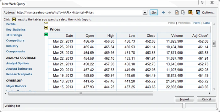
2. A browser window named “New Web Query” will appear.

3. In the address bar, write the web address.

 (picture from excel-university.com)

4. The page will load and will show yellow icons against data/tables.

5. Select the appropriate one.

6. Press the Import button.

Now you have the web data scraped into the Excel Worksheet — perfectly arranged in rows and columns as you like.

Scrape Web Data with Excel VBA

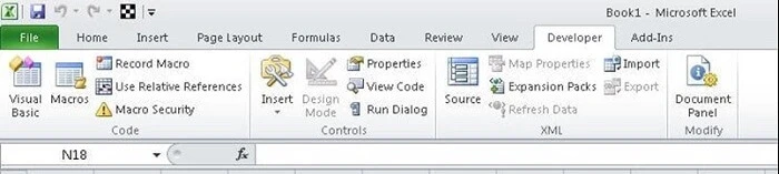
Most of us would use formula’s in Excel (e.g. =avg(…), =sum(…), =if(…), etc.) a lot, but are less familiar with the built-in language — Visual Basic for Application a.k.a VBA. It’s commonly known as “Macros” and such Excel files are saved as a **.xlsm. Before using it, you need to first enable the Developer tab in the ribbon (right-click File -> Customize Ribbon -> check Developer tab). Then set up your layout. In this developer interface, you can write VBA code attached to various events. Click HERE (https://msdn.microsoft.com/en-us/library/office/ee814737(v=office.14).aspx) to getting started with VBA in Excel 2010.

Using Excel VBA is going to be a bit technical — this is not very friendly for non-programmers among us. VBA works by running macros, step-by-step procedures written in Excel Visual Basic. To scrape data from websites to Excel using VBA, we need to build or get some VBA script to send some requests to web pages and get returned data from these web pages. It’s common to use VBA with XML HTTP and regular expressions to parse the web pages. For Windows, you can use VBA with Win HTTP or Internet Explorer to scrape data from websites to Excel.

With some patience and some practice, you would find it worthwhile to learn some Excel VBA code and some HTML knowledge to make your web scraping into Excel much easier and more efficient for automating the repetitive work. There’s a plentiful amount of material and forums for you to learn how to write VBA code.

Top 20 Web Crawling Tools for Extracting Web Data

Top 30 Free Web Scraping Software

10 Simple Excel Functions for Data Analysis

How to Extract Data from PDF to Excel

In this tutorial, we will show you different ways to fetch data from a website into excel automatically. This is often one of the foremost used excel features for those that use excel for data analysis work.

Follow the below step-by-step procedure to learn how to fetch data directly and skip the hassle of doing data entry manually from a website.

Extracting data (data collection and update) automatically from a webpage to your Excel worksheet could be
important for a few jobs. Let’s see how you can do it.

Method 1: Copy – Paste (One time + Manual)

This method is the easiest as it enables direct data fetching in the literal sense.

To do so:

• Simply open the website from where we would like to seek information.
• Copy the data which we want to have in our Excel sheet
• Select the tabular column (or Cell) and Paste it to get the web data into your Excel sheet.

As this method fetches the data only once, the drawback of this method is that you simply cannot refresh the information fetched timely when the changes are made within the website then again you would require to repeat the above step to keep your worksheet updated.

Method 2: Realtime Data Extraction

We will be using Excel’s From Web Command within the Data ribbon to gather data from the website. Say, I would like to
gather data from the below page or URL: https://economictimes.indiatimes.com/wealth/fuel-price/petrol.

It shows the daily Petrol-Price’s for respective cities, all over India. To fetch the data directly into our Excel sheets we follow the below steps:

• In the Excel worksheet, open the Data ribbon and click on the From Web command.

• A New Web Query dialog box appears
• In the address bar, I have pasted the address URL of our desired webpage (you must paste accordingly): https://economictimes.indiatimes.com/wealth/fuel-price/petrol.
• Then Click on the Go button, placed right after the address bar

• The same website loads up within the new web query panel as a preview.
• Now spot the yellow arrows near the query box.

• Move your mouse pointer over the yellow arrows. You see a zone is highlighted with a blue border and therefore the yellow arrow becomes green on hover.

In our example, I have chosen the City wise petrol prices all over India.

• Now, Click on the Import button. Import Data panel appears. It asks about the location of importing the data, currently, I choose to reserve it in cell A1, but you may reserve it anywhere, in any cell of the worksheet.

As we see now that the info required by us is inserted into the excel worksheet. Now as we’ve got the info we will make
changes as we would like as per our requirement.

NOTE:- The website should have data in a format like Table or Pre-data format. Otherwise, it increases the work because
then we need to convert the data into a readable or excel-able format which again is a bit hectic.

After all the text shown in the columns isn’t your ally. So, we shall assume your life is straightforward like that and you’ve got an internet site that has data in a compatible direct Excel readable format.

The other most important thing is that you need not have to update the data from time to time.

Refresh Excel data for Update:

You can manually or automatically refresh the data. To do so click on the drop-down button of the refresh all command.

You can click on Refresh if you need just one cell to update and Refresh All if you want everything in the sheet to re-fetch data.

We can even set a period time for refreshing data automatically. Click on this Connection Properties option from the list.

You can name the connection, add an outline too.

Under Refresh Control, you get a command Refresh every (by default 60 minutes), which is subject to configuration.

Conclusion

So that’s it for this tutorial, hope you’ve got understood the way to pull/extract the data from the website into an Excel
sheet.