Data commands in excel - Word и Excel - помощь в работе с программами

Below is a brief overview of about 100 important Excel functions you should know, with links to detailed examples. We also have a large list of example formulas, a more complete list of Excel functions, and video training. If you are new to Excel formulas, see this introduction.

Note: Excel now includes Dynamic Array formulas, which offer important new functions.

Date and Time Functions

Excel provides many functions to work with dates and times.

NOW and TODAY

You can get the current date with the TODAY function and the current date and time with the NOW Function. Technically, the NOW function returns the current date and time, but you can format as time only, as seen below:

TODAY() // returns current date
NOW() // returns current time

Note: these are volatile functions and will recalculate with every worksheet change. If you want a static value, use date and time shortcuts.

DAY, MONTH, YEAR, and DATE

You can use the DAY, MONTH, and YEAR functions to disassemble any date into its raw components, and the DATE function to put things back together again.

=DAY("14-Nov-2018") // returns 14
=MONTH("14-Nov-2018") // returns 11
=YEAR("14-Nov-2018") // returns 2018
=DATE(2018,11,14) // returns 14-Nov-2018

HOUR, MINUTE, SECOND, and TIME

Excel provides a set of parallel functions for times. You can use the HOUR, MINUTE, and SECOND functions to extract pieces of a time, and you can assemble a TIME from individual components with the TIME function.

=HOUR("10:30") // returns 10
=MINUTE("10:30") // returns 30
=SECOND("10:30") // returns 0
=TIME(10,30,0) // returns 10:30

DATEDIF and YEARFRAC

You can use the DATEDIF function to get time between dates in years, months, or days. DATEDIF can also be configured to get total time in «normalized» denominations, i.e. «2 years and 6 months and 27 days».

Use YEARFRAC to get fractional years:

=YEARFRAC("14-Nov-2018","10-Jun-2021") // returns 2.57

EDATE and EOMONTH

A common task with dates is to shift a date forward (or backward) by a given number of months. You can use the EDATE and EOMONTH functions for this. EDATE moves by month and retains the day. EOMONTH works the same way, but always returns the last day of the month.

EDATE(date,6) // 6 months forward
EOMONTH(date,6) // 6 months forward (end of month)

WORKDAY and NETWORKDAYS

To figure out a date n working days in the future, you can use the WORKDAY function. To calculate the number of workdays between two dates, you can use NETWORKDAYS.

WORKDAY(start,n,holidays) // date n workdays in future

Video: How to calculate due dates with WORKDAY

NETWORKDAYS(start,end,holidays) // number of workdays between dates

Note: Both functions automatically skip weekends (Saturday and Sunday) and will also skip holidays, if provided. If you need more flexibility on what days are considered weekends, see the WORKDAY.INTL function and NETWORKDAYS.INTL function.

WEEKDAY and WEEKNUM

To figure out the day of week from a date, Excel provides the WEEKDAY function. WEEKDAY returns a number between 1-7 that indicates Sunday, Monday, Tuesday, etc. Use the WEEKNUM function to get the week number in a given year.

=WEEKDAY(date) // returns a number 1-7
=WEEKNUM(date) // returns week number in year

Engineering

CONVERT

Most Engineering functions are pretty technical…you’ll find a lot of functions for complex numbers in this section. However, the CONVERT function is quite useful for everyday unit conversions. You can use CONVERT to change units for distance, weight, temperature, and much more.

=CONVERT(72,"F","C") // returns 22.2

Information Functions

ISBLANK, ISERROR, ISNUMBER, and ISFORMULA

Excel provides many functions for checking the value in a cell, including ISNUMBER, ISTEXT, ISLOGICAL, ISBLANK, ISERROR, and ISFORMULA These functions are sometimes called the «IS» functions, and they all return TRUE or FALSE based on a cell’s contents.

Excel also has ISODD and ISEVEN functions that will test a number to see if it’s even or odd.

By the way, the green fill in the screenshot above is applied automatically with a conditional formatting formula.

Logical Functions

Excel’s logical functions are a key building block of many advanced formulas. Logical functions return the boolean values TRUE or FALSE. If you need a primer on logical formulas, this video goes through many examples.

AND, OR and NOT

The core of Excel’s logical functions are the AND function, the OR function, and the NOT function. In the screen below, each of these function is used to run a simple test on the values in column B:

=AND(B5>3,B5<9)
=OR(B5=3,B5=9)
=NOT(B5=2)

Video: How to build logical formulas
Guide: 50 examples of formula criteria

IFERROR and IFNA

The IFERROR function and IFNA function can be used as a simple way to trap and handle errors. In the screen below, VLOOKUP is used to retrieve cost from a menu item. Column F contains just a VLOOKUP function, with no error handling. Column G shows how to use IFNA with VLOOKUP to display a custom message when an unrecognized item is entered.

=VLOOKUP(E5,menu,2,0) // no error trapping
=IFNA(VLOOKUP(E5,menu,2,0),"Not found") // catch errors

Whereas IFNA only catches an #N/A error, the IFERROR function will catch any formula error.

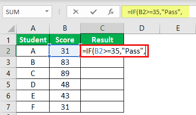
IF and IFS functions

The IF function is one of the most used functions in Excel. In the screen below, IF checks test scores and assigns «pass» or «fail»:

Multiple IF functions can be nested together to perform more complex logical tests.

New in Excel 2019 and Excel 365, the IFS function can run multiple logical tests without nesting IFs.

=IFS(C5<60,"F",C5<70,"D",C5<80,"C",C5<90,"B",C5>=90,"A")

Lookup and Reference Functions

VLOOKUP and HLOOKUP

Excel offers a number of functions to lookup and retrieve data. Most famous of all is VLOOKUP:

=VLOOKUP(C5,$F$5:$G$7,2,TRUE)

More: 23 things to know about VLOOKUP.

HLOOKUP works like VLOOKUP, but expects data arranged horizontally:

=HLOOKUP(C5,$G$4:$I$5,2,TRUE)

INDEX and MATCH

For more complicated lookups, INDEX and MATCH offers more flexibility and power:

=INDEX(C5:E12,MATCH(H4,B5:B12,0),MATCH(H5,C4:E4,0))

Both the INDEX function and the MATCH function are powerhouse functions that turn up in all kinds of formulas.

More: How to use INDEX and MATCH

LOOKUP

The LOOKUP function has default behaviors that make it useful when solving certain problems. LOOKUP assumes values are sorted in ascending order and always performs an approximate match. When LOOKUP can’t find a match, it will match the next smallest value. In the example below we are using LOOKUP to find the last entry in a column:

ROW and COLUMN

You can use the ROW function and COLUMN function to find row and column numbers on a worksheet. Notice both ROW and COLUMN return values for the current cell if no reference is supplied:

The row function also shows up often in advanced formulas that process data with relative row numbers.

ROWS and COLUMNS

The ROWS function and COLUMNS function provide a count of rows in a reference. In the screen below, we are counting rows and columns in an Excel Table named «Table1».

Note ROWS returns a count of data rows in a table, excluding the header row. By the way, here are 23 things to know about Excel Tables.

HYPERLINK

You can use the HYPERLINK function to construct a link with a formula. Note HYPERLINK lets you build both external links and internal links:

=HYPERLINK(C5,B5)

GETPIVOTDATA

The GETPIVOTDATA function is useful for retrieving information from existing pivot tables.

=GETPIVOTDATA("Sales",$B$4,"Region",I6,"Product",I7)

CHOOSE

The CHOOSE function is handy any time you need to make a choice based on a number:

=CHOOSE(2,"red","blue","green") // returns "blue"

Video: How to use the CHOOSE function

TRANSPOSE

The TRANSPOSE function gives you an easy way to transpose vertical data to horizontal, and vice versa.

{=TRANSPOSE(B4:C9)}

Note: TRANSPOSE is a formula and is, therefore, dynamic. If you just need to do a one-time transpose operation, use Paste Special instead.

OFFSET

The OFFSET function is useful for all kinds of dynamic ranges. From a starting location, it lets you specify row and column offsets, and also the final row and column size. The result is a range that can respond dynamically to changing conditions and inputs. You can feed this range to other functions, as in the screen below, where OFFSET builds a range that is fed to the SUM function:

=SUM(OFFSET(B4,1,I4,4,1)) // sum of Q3

INDIRECT

The INDIRECT function allows you to build references as text. This concept is a bit tricky to understand at first, but it can be useful in many situations. Below, we are using INDIRECT to get values from cell A1 in 5 different worksheets. Each reference is dynamic. If a sheet name changes, the reference will update.

=INDIRECT(B5&"!A1") // =Sheet1!A1

The INDIRECT function is also used to «lock» references so they won’t change, when rows or columns are added or deleted. For more details, see linked examples at the bottom of the INDIRECT function page.

Caution: both OFFSET and INDIRECT are volatile functions and can slow down large or complicated spreadsheets.

STATISTICAL Functions

COUNT and COUNTA

You can count numbers with the COUNT function and non-empty cells with COUNTA. You can count blank cells with COUNTBLANK, but in the screen below we are counting blank cells with COUNTIF, which is more generally useful.

=COUNT(B5:F5) // count numbers
=COUNTA(B5:F5) // count numbers and text
=COUNTIF(B5:F5,"") // count blanks

COUNTIF and COUNTIFS

For conditional counts, the COUNTIF function can apply one criteria. The COUNTIFS function can apply multiple criteria at the same time:

=COUNTIF(C5:C12,"red") // count red
=COUNTIF(F5:F12,">50") // count total > 50
=COUNTIFS(C5:C12,"red",D5:D12,"TX") // red and tx
=COUNTIFS(C5:C12,"blue",F5:F12,">50") // blue > 50

Video: How to use the COUNTIF function

SUM, SUMIF, SUMIFS

To sum everything, use the SUM function. To sum conditionally, use SUMIF or SUMIFS. Following the same pattern as the counting functions, the SUMIF function can apply only one criteria while the SUMIFS function can apply multiple criteria.

=SUM(F5:F12) // everything
=SUMIF(C5:C12,"red",F5:F12) // red only
=SUMIF(F5:F12,">50") // over 50
=SUMIFS(F5:F12,C5:C12,"red",D5:D12,"tx") // red & tx
=SUMIFS(F5:F12,C5:C12,"blue",F5:F12,">50") // blue & >50

Video: How to use the SUMIF function

AVERAGE, AVERAGEIF, and AVERAGEIFS

Following the same pattern, you can calculate an average with AVERAGE, AVERAGEIF, and AVERAGEIFS.

=AVERAGE(F5:F12) // all
=AVERAGEIF(C5:C12,"red",F5:F12) // red only
=AVERAGEIFS(F5:F12,C5:C12,"red",D5:D12,"tx") // red and tx

MIN, MAX, LARGE, SMALL

You can find largest and smallest values with MAX and MIN, and nth largest and smallest values with LARGE and SMALL. In the screen below, data is the named range C5:C13, used in all formulas.

=MAX(data) // largest
=MIN(data) // smallest
=LARGE(data,1) // 1st largest
=LARGE(data,2) // 2nd largest
=LARGE(data,3) // 3rd largest
=SMALL(data,1) // 1st smallest
=SMALL(data,2) // 2nd smallest
=SMALL(data,3) // 3rd smallest

Video: How to find the nth smallest or largest value

MINIFS, MAXIFS

The MINIFS and MAXIFS. These functions let you find minimum and maximum values with conditions:

=MAXIFS(D5:D15,C5:C15,"female") // highest female
=MAXIFS(D5:D15,C5:C15,"male") // highest male
=MINIFS(D5:D15,C5:C15,"female") // lowest female
=MINIFS(D5:D15,C5:C15,"male") // lowest male

Note: MINIFS and MAXIFS are new in Excel via Office 365 and Excel 2019.

MODE

The MODE function returns the most commonly occurring number in a range:

=MODE(B5:G5) // returns 1

RANK

To rank values largest to smallest, or smallest to largest, use the RANK function:

Video: How to rank values with the RANK function

MATH Functions

ABS

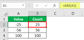
To change negative values to positive use the ABS function.

=ABS(-134.50) // returns 134.50

RAND and RANDBETWEEN

Both the RAND function and RANDBETWEEN function can generate random numbers on the fly. RAND creates long decimal numbers between zero and 1. RANDBETWEEN generates random integers between two given numbers.

=RAND() // between zero and 1
=RANDBETWEEN(1,100) // between 1 and 100

ROUND, ROUNDUP, ROUNDDOWN, INT

To round values up or down, use the ROUND function. To force rounding up to a given number of digits, use ROUNDUP. To force rounding down, use ROUNDDOWN. To discard the decimal part of a number altogether, use the INT function.

=ROUND(11.777,1) // returns 11.8
=ROUNDUP(11.777) // returns 11.8
=ROUNDDOWN(11.777,1) // returns 11.7
=INT(11.777) // returns 11

MROUND, CEILING, FLOOR

To round values to the nearest multiple use the MROUND function. The FLOOR function and CEILING function also round to a given multiple. FLOOR forces rounding down, and CEILING forces rounding up.

=MROUND(13.85,.25) // returns 13.75
=CEILING(13.85,.25) // returns 14
=FLOOR(13.85,.25) // returns 13.75

MOD

The MOD function returns the remainder after division. This sounds boring and geeky, but MOD turns up in all kinds of formulas, especially formulas that need to do something «every nth time». In the screen below, you can see how MOD returns zero every third number when the divisor is 3:

SUMPRODUCT

The SUMPRODUCT function is a powerful and versatile tool when dealing with all kinds of data. You can use SUMPRODUCT to easily count and sum based on criteria, and you can use it in elegant ways that just don’t work with COUNTIFS and SUMIFS. In the screen below, we are using SUMPRODUCT to count and sum orders in March. See the SUMPRODUCT page for details and links to many examples.

=SUMPRODUCT(--(MONTH(B5:B12)=3)) // count March
=SUMPRODUCT(--(MONTH(B5:B12)=3),C5:C12) // sum March

SUBTOTAL

The SUBTOTAL function is an «aggregate function» that can perform a number of operations on a set of data. All told, SUBTOTAL can perform 11 operations, including SUM, AVERAGE, COUNT, MAX, MIN, etc. (see this page for the full list). The key feature of SUBTOTAL is that it will ignore rows that have been «filtered out» of an Excel Table, and, optionally, rows that have been manually hidden. In the screen below, SUBTOTAL is used to count and sum only the 7 visible rows in the table:

=SUBTOTAL(3,B5:B14) // returns 7
=SUBTOTAL(9,F5:F14) // returns 9.54

AGGREGATE

Like SUBTOTAL, the AGGREGATE function can also run a number of aggregate operations on a set of data and can optionally ignore hidden rows. The key differences are that AGGREGATE can run more operations (19 total) and can also ignore errors.

In the screen below, AGGREGATE is used to perform MIN, MAX, LARGE and SMALL operations while ignoring errors. Normally, the error in cell B9 would prevent these functions from returning a result. See this page for a full list of operations AGGREGATE can perform.

=AGGREGATE(4,6,values) // MAX ignore errors, returns 100
=AGGREGATE(5,6,values) // MIN ignore errors, returns 75

TEXT Functions

LEFT, RIGHT, MID

To extract characters from the left, right, or middle of text, use LEFT, RIGHT, and MID functions:

=LEFT("ABC-1234-RED",3) // returns "ABC"
=MID("ABC-1234-RED",5,4) // returns "1234"
=RIGHT("ABC-1234-RED",3) // returns "RED"

LEN

The LEN function will return the length of a text string. LEN shows up in a lot of formulas that count words or characters.

FIND, SEARCH

To look for specific text in a cell, use the FIND function or SEARCH function. These functions return the numeric position of matching text, but SEARCH allows wildcards and FIND is case-sensitive. Both functions will throw an error when text is not found, so wrap in the ISNUMBER function to return TRUE or FALSE (example here).

=FIND("Better the devil you know","devil") // returns 12
=SEARCH("This is not my beautiful wife","bea*") // returns 12

REPLACE, SUBSTITUTE

To replace text by position, use the REPLACE function. To replace text by matching, use the SUBSTITUTE function. In the first example, REPLACE removes the two asterisks (**) by replacing the first two characters with an empty string («»). In the second example, SUBSTITUTE removes all hash characters (#) by replacing «#» with «».

=REPLACE("**Red",1,2,"") // returns "Red"
=SUBSTITUTE("##Red##","#","") // returns "Red"

CODE, CHAR

To figure out the numeric code for a character, use the CODE function. To translate the numeric code back to a character, use the CHAR function. In the example below, CODE translates each character in column B to its corresponding code. In column F, CHAR translates the code back to a character.

=CODE("a") // returns 97
=CHAR(97) // returns "a"

Video: How to use the CODE and CHAR functions

TRIM, CLEAN

To get rid of extra space in text, use the TRIM function. To remove line breaks and other non-printing characters, use CLEAN.

=TRIM(A1) // remove extra space
=CLEAN(A1) // remove line breaks

Video: How to clean text with TRIM and CLEAN

CONCAT, TEXTJOIN, CONCATENATE

New in Excel via Office 365 are CONCAT and TEXTJOIN. The CONCAT function lets you concatenate (join) multiple values, including a range of values without a delimiter. The TEXTJOIN function does the same thing, but allows you to specify a delimiter and can also ignore empty values.

=TEXTJOIN(",",TRUE,B4:H4) // returns "red,blue,green,pink,black"
=CONCAT(B7:H7) // returns "8675309"

Excel also provides the CONCATENATE function, but it doesn’t offer special features. I wouldn’t bother with it and would instead concatenate directly with the ampersand (&) character in a formula.

EXACT

The EXACT function allows you to compare two text strings in a case-sensitive manner.

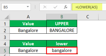
UPPER, LOWER, PROPER

To change the case of text, use the UPPER, LOWER, and PROPER function

=UPPER("Sue BROWN") // returns "SUE BROWN"
=LOWER("Sue BROWN") // returns "sue brown"
=PROPER("Sue BROWN") // returns "Sue Brown"

Video: How to change case with formulas

TEXT

Last but definitely not least is the TEXT function. The text function lets you apply number formatting to numbers (including dates, times, etc.) as text. This is especially useful when you need to embed a formatted number in a message, like «Sale ends on [date]».

=TEXT(B5,"$#,##0.00") 
=TEXT(B6,"000000")
="Save "&TEXT(B7,"0%")
="Sale ends "&TEXT(B8,"mmm d")

More: Detailed examples of custom number formatting.

Dynamic Array functions

Dynamic arrays are new in Excel 365, and are a major upgrade to Excel’s formula engine. As part of the dynamic array update, Excel includes new functions which directly leverage dynamic arrays to solve problems that are traditionally hard to solve with conventional formulas. If you are using Excel 365, make sure you are aware of these new functions:

Function	Purpose
FILTER	Filter data and return matching records
RANDARRAY	Generate array of random numbers
SEQUENCE	Generate array of sequential numbers
SORT	Sort range by column
SORTBY	Sort range by another range or array
UNIQUE	Extract unique values from a list or range
XLOOKUP	Modern replacement for VLOOKUP
XMATCH	Modern replacement for the MATCH function

Video: New dynamic array functions in Excel (about 3 minutes).

Quick navigation

ABS, AGGREGATE, AND, AVERAGE, AVERAGEIF, AVERAGEIFS, CEILING, CHAR, CHOOSE, CLEAN, CODE, COLUMN, COLUMNS, CONCAT, CONCATENATE, CONVERT, COUNT, COUNTA, COUNTBLANK, COUNTIF, COUNTIFS, DATE, DATEDIF, DAY, EDATE, EOMONTH, EXACT, FIND, FLOOR, GETPIVOTDATA, HLOOKUP, HOUR, HYPERLINK, IF, IFERROR, IFNA, IFS, INDEX, INDIRECT, INT, ISBLANK, ISERROR, ISEVEN, ISFORMULA, ISLOGICAL, ISNUMBER, ISODD, ISTEXT, LARGE, LEFT, LEN, LOOKUP, LOWER, MATCH, MAX, MAXIFS, MID, MIN, MINIFS, MINUTE, MOD, MODE, MONTH, MROUND, NETWORKDAYS, NOT, NOW, OFFSET, OR, PROPER, RAND, RANDBETWEEN, RANK, REPLACE, RIGHT, ROUND, ROUNDDOWN, ROUNDUP, ROW, ROWS, SEARCH, SECOND, SMALL, SUBSTITUTE, SUBTOTAL, SUM, SUMIF, SUMIFS, SUMPRODUCT, TEXT, TEXTJOIN, TIME, TODAY, TRANSPOSE, TRIM, UPPER, VLOOKUP, WEEKDAY, WEEKNUM, WORKDAY, YEAR, YEARFRAC

Источник

List of Top 10 Commands in Excel

Whether in engineering, medicine, chemistry, or any field, an Excel spreadsheet is the common tool for data maintenance. Some of them use it to maintain their database and others use this tool as a weapon to turn fortune for the respective companies they are working on. So, you, too, can turn things around for yourself by learning some of the most useful Excel commands.

List of Top 10 Commands in Excel
- #1 VLOOKUP Function to Fetch Data
- #2 IF Condition to Do Logical Test
- #3 CONCATENATE Function to Combine Two or More Values
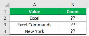
- #4 Count Only Numerical Values
- #5 Count All Values
- #6 Count Based on Condition
- #7 Count Number of Characters in the Cell
- #8 Convert Negative Value to Positive Value
- #9 Convert All Characters to UPPERCASE Values
- #10 Find Maximum and Minimum Values
- Things to Remember
- Recommended Articles

You can download this Commands in Excel Template here – Commands in Excel Template

#1 VLOOKUP Function to Fetch Data

The data in multiple sheets are common in many offices, but fetching the data from one worksheet to another and from one workbook to another is a challenge for beginners in Excel.

If you have struggled to fetch the data, VLOOKUPThe VLOOKUP excel function searches for a particular value and returns a corresponding match based on a unique identifier. A unique identifier is uniquely associated with all the records of the database. For instance, employee ID, student roll number, customer contact number, seller email address, etc., are unique identifiers.
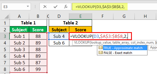
read more will help you bring the data. For example, assume you have two tables below.

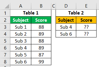
In table 1, we have the subject list and their respective scores, and in table 2, we have some subject names, but we do not have scores for them. So, using these subject names in table 2, we need to fetch the data from table 1.

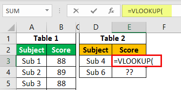
First, let us open the VLOOKUP function in the E2 cell.
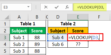
Then, select the LOOKUP value as a D3 cell.
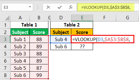
Next, we must select the table array as A3 to B8 and press the F4 key to make them an absolute reference.
Column Index Number is from the selected table array from which column you need to fetch the data. So, in this case, from the second column, we need to bring the data.
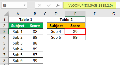
For the last argument range, LOOKUP, we must select FALSE as the option, or else we can enter.
Close the bracket and press the Enter key to get the score of Sub 4. Also, copy the formula and paste it to the below cell.

You have learned a formula to fetch values from different tables based on a LOOKUP value.

#2 IF Condition to Do Logical Test

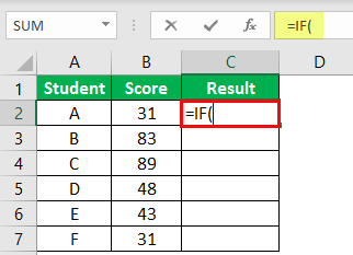
The Excel IF condition can be your friend in many situations because of its ability to conduct logical tests. For example, assume you want to test the scores of students and give the result. Below is the data for your reference.

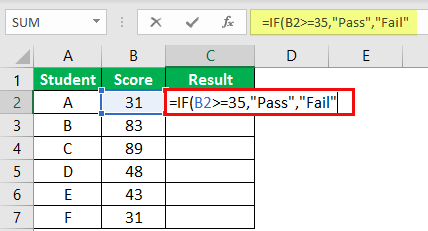
In the above table, we have students’ scores from the examination. So we need to arrive at the result as either “PASS” or “FAIL” based on these scores. So to reach these results criteria, if the score is >=35, the result should be “PASS” or else “FAIL.”

We must first open the IF condition in the C2 cell.

The first argument is logical to test.So, in this example, we need to do the logical test of whether the score is >=35, select the score cell B2, and apply the logical test as B2 >= 35.

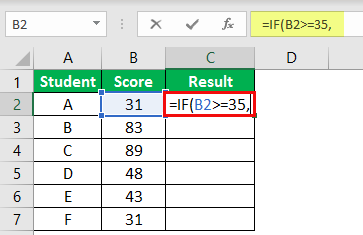
The next argument is value if true. If the applied logical test is “TRUE,” what is the value we need? If the logical test is “TRUE,” we need the result as “Pass.”

So, the final part is value if false.If the applied logical test is “FALSE,” then we need the result as “Fail.”

Now, close the bracket, and we also need to fill the formula to the remaining cells.

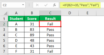
So, students A and F scored less than 35. Therefore, the result has arrived as “FAIL.”

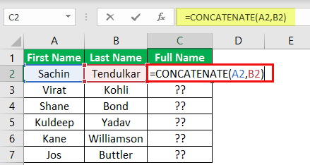
#3 CONCATENATE Function to Combine Two or More Values

If we want to combine two or more values from different cells, we can use the CONCATENATE function in excelThe CONCATENATE function in Excel helps the user concatenate or join two or more cell values which may be in the form of characters, strings or numbers.read more. For example, below is the “First Name” list and “Last Name.”

First, we need to open the CONCATENATE function in the C2 cell.

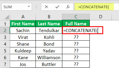
For the first argument, “Text 1,“ select the “First Name” cell, and for “Text 2,” choose the “Last Name” cell.

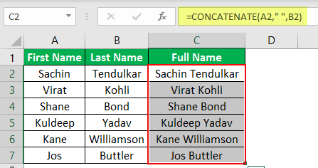
Then, we need to apply the formula to all the cells to get the full name.

If you want space as the “First Name” and “Last Name” separator, we can use the space character in double-quotes after selecting the first name.

#4 Count Only Numerical Values

If we want to count only numerical values from the range, you need to use the COUNT function in Excel. Take a look at the below data.

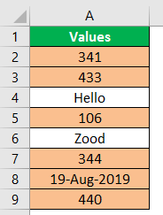
From the above table, we need to count only numerical values. For this, we can use the COUNT function.

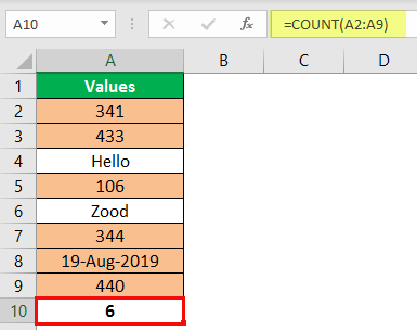
The result of the COUNT function is 6. The total count of cells is 8, but we have got the count of numerical values as 6. In cells A4 and A6, we have text values, but in cell A8, we have date values. The Excel COUNT function treats the date also as a numerical value only.

Note: “Date” and “Time” values are numerical values if the formatting is correct. Otherwise, they will be treated as “text” values.

#5 Count All Values

If we want to count all the values in the range, we need to use the COUNTA functionThe COUNTA function is an inbuilt statistical excel function that counts the number of non-blank cells (not empty) in a cell range or the cell reference. For example, cells A1 and A3 contain values but, cell A2 is empty. The formula “=COUNTA(A1,A2,A3)” returns 2.
read more. We will apply the COUNTA function for the same data and see the count.

We got the count as 8 because the COUNTA function has counted all the cell values.

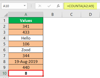
Note: Both the COUNT and COUNTA functions ignore blank cells.

#6 Count Based on Condition

If we want to count based on condition, we can use the COUNTIF functionThe COUNTIF function in Excel counts the number of cells within a range based on pre-defined criteria. It is used to count cells that include dates, numbers, or text. For example, COUNTIF(A1:A10,”Trump”) will count the number of cells within the range A1:A10 that contain the text “Trump”
read more. For example, look at the below data.

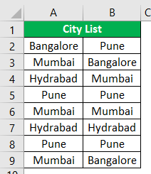
From this “City List,” if we want to count how many times “Bangalore” city is mentioned, we must open the COUNTIF function.

The first argument is “RANGE,” so we need to select the range of values from A2 to B9.

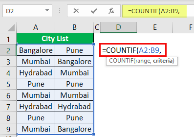
The second argument is “Criteria,” i.e., what you want to count, i.e., “Bangalore.

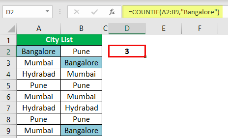
Bangalore has appeared three times in the range A2 to B9, so the COUNTIF function returns 3 as the count.

#7 Count Number of Characters in the Cell

If we want to count the number of characters in the cell, we need to use the LEN function in excelThe Len function returns the length of a given string. It calculates the number of characters in a given string as input. It is a text function in Excel as well as an inbuilt function that can be accessed by typing =LEN( and entering a string as input.read moreel. The LEN function returns the number of characters from the selected cell.

“Excel” has 5 characters, so the result is 5.

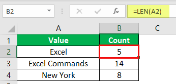
Note: Space is also considered as one character.

#8 Convert Negative Value to Positive Value

If we have negative values and want to convert them to positive ones, the ABS functionABS Excel function or Absolute function is used to calculate the absolute value of a given number. The negative numbers given as input are changed to positive numbers and if the argument provided to this function is positive, it remains unchanged.read more can do it for us.

#9 Convert All Characters to UPPERCASE Values

If we want to convert all the text values to UPPERCASE, we can use the UPPER formula in excelUppercase function in Excel is used to convert lowercase text to uppercase.read more.

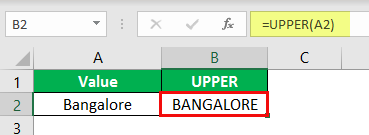
And if we want to convert all the text values to LOWERCASE values, then use the LOWER formula.

#10 Find Maximum and Minimum Values

If we want to find maximum and minimum values, we may use MAX and MIN functions in excelIn Excel, the MIN function is categorized as a statistical function. It finds and returns the minimum value from a given set of data/array.read more, respectively.

Things to Remember

These are some of the important formulas/commands in excel which are used regularly.
We can also use these functions at the advanced level.
There are more advanced formulas in Excel which come under advanced level courses.
Space is considered one character.

Excel Advanced
Concepts
By J. Carlton Collins

Presented below are some of the more advanced concepts,
topics and bullet points I like to cover in my Advanced excel courses.

The
Data Menu — Perhaps the parts
of Excel that are of most value to CPAs, but least used by CPAs are the Data
commands found under the Data menu in Excel 2003 and earlier, and on the data
Ribbon in Excel 2007. These commands are shown below, and we will concentrate
the next hour to studying these commands.

Data Sort — The Sort tool
does exactly what it implies � it sorts and data. Key sorting points are as
follows:

1.
Contiguous Data
— The �A to Z� sorting tool can sort large matrix of data automatically as long
as the data is contiguous. In other words, your data should contain no blank
columns, no blank rows, and the columns must all be labeled. Only then will
Excel always correctly select the entire matrix for sorting.

2.
A to Z Button
— Simply place the cursor in the desired column for sorted, and press the A to Z
or Z to A button as the case may be. Excel will automatically sort all
continuous columns that have headings and all contiguous rows from the top row
under the heading labels down to the last row in the selected column that
contains data. (Note — If you accidently select 2 cells instead of just one,
your results will not be correct.)

3.
Sort by 64
Columns — The �Sort� tool is
dramatically enhanced in Excel 2007 as it now provides the ability to sort by up
to 64 columns, instead of just 3 columns. Presented below is a dialog box which
shows this expanded functionality.

4.
Sort Left to
Right � Excel has always provided the
ability to sort left to right. To do so, select the options box in the Sort
Dialog box and click the check box labeled �Sort left to Right� as shown below.

5.
Sort by Color
� Excel 2007 now provides the ability to sort by font color or by cell color, or
both. This is handy in many ways. Sometimes CPAs use color to tag or mark
certain cells — and later find it useful to be able to sort by those markings.
In other situations CPAs use conditional formatting to apply color to cells
using a wide variety of rules. Thereafter Excel can sort the data based on the
resulting colors. The sort-by-color options are shown below.

To be accurate, it was
possible to sort by color in Excel 2003. To accomplish this task, you needed to
use the =CELL function in order to identify information about a given cell such
as the cell color or font color. Thereafter, the results of that function could
be used to sort rows � which effectively means that you can sort by color in
Excel 2003 � but it takes a bit more effort.

6.
Sort By Custom
List � Another sorting capability in
Excel is the ability to sort by Custom List. For example, assume a CPA firm has
ten partners, and the Managing partner prefers to be shown at the top of the
list, and the remaining Partners based on seniority. In this case, you could
create a Custom List in the excel Options dialog box listing the partners in the
desired order, and then sort future reports based on that order.

Perhaps a better example
use of this feature would be to create a non-alphabetic custom list of your
chart of accounts, and then sort transactions to produce a general ledger in
chart of account order � even if your preferred chart of accounts is not
alphabetical. the partner seniority does not match the alphabetic names,
nor any

Filtering Data
— Using AutoFilter to filter data allows you to view a subset of your data in a
range of cells or table. Once you have filtered the data, you can apply
additional filters to further refine your data view. When you are done, you can
clear a filter to once again redisplay all of the data. To use this tool, start
with any list of data and turn on the AutoFilter tool. Then position your cursor
in the column you want to filter and use the drop down arrows to apply your
filters as shown in the screen below.

Once the filters are applied, you will see a
subset your data. For example, the screen presented below shows filtered data
for only Macon and Savannah properties.

As filters are applied, a small funnel appears in
the drop down arrow button to indicate that a filter has been applied. You can
apply filters for multiple columns simultaneously.

Key Points Concerning The
AutoFilter Command:

1.
Contiguous Data
� The AutoFilter tools works best when you are working with data that is
contiguous. In other words, your data should contain no blank columns, no blank
rows, and the columns must all be labeled.

2.
Filter by
Multiple Columns — You can filter by
more than one column.

3.
Removing Filters
� In Excel 2003 and earlier, a faster way to remove multiple filters is to turn
off filtering and then turn filtering back on. In Excel 2007 you can simple
click the Clear button in the Sort and Filter Group as shown below.

4.
Filters are
Additive — Each additional filter is
based on the current filter and further reduces the subset of data.

5.
Three Types of
Filters � You can filter based on
list values, by formats, or by criteria. Each of these filter types is mutually
exclusive for each range of cells or column table. For example, you can filter
by cell color or by a list of numbers, but not by both; you can filter by icon
or by a custom filter, but not by both.

6.
Filters Enabled —
A drop-down arrow means that filtering is enabled but not
applied.

7.
Filter Applied —
A Filter button means
that a filter is applied.

8.
Filter Spanning
— The commands under the All Dates in the Period menu, such as January or
Quarter 2, filter by the period no matter what the year. This can be useful, for
example, to compare sales by a period across several years.

9.
This Year vs.
Year-to-Date Filtering — This Year
and Year-to-Date are different in the way that future dates are handled. This
Year can return dates in the future for the current year, whereas Year to Date
only returns dates up to and including the current date.

10.
Filtering Dates
— All date filters are based on the Gregorian calendar as decreed by Pope
Gregory XIII, after whom the calendar was named, on 24 February 1582. The
Gregorian calendar modifies the Julian calendar’s regular four-year cycle of
leap years as follows: Every year that is exactly divisible by four is a leap
year, except for years that are exactly divisible by 100; the centurial years
that are exactly divisible by 400 are still leap years. For example, the year
1900 is not a leap year; the year 2000 is a leap year.

11.
Filtering By Days
of Week — If you want to filter by
days of the week, simply format the cells to show the day of the week.

12.
Top & Bottom
Filtering — On the Data tab, in the
Sort & Filter group, click Filter. Point to Number Filters and then select Top
10. To filter by number, click Items. To filter by percentage, click Percent.
Note — Top and bottom values are based on the original range of cells or table
column and not the filtered subset of data.

13.
Above & Below
Average Filtering — On the Data tab,
in the Sort & Filter group, click Filter. Point to Filter by Numbers that are
Above/Below Average. Note � These values are based on the original range of
cells or table column and not the filtered subset of data.

14.
Filtering Out
Blanks — To filter for blanks, in the
AutoFilter menu at the top of the list of values, clear (Select All), and then
at the bottom of the list of values, select (Blanks).

15.
Filtering By
Color — Select Filter by Color, and
then depending on the type of format, select Filter by Cell Color, Filter by
Font Color, or Filter by Cell Icon.

16.
Filter by
Selection — To filter by text,
number, or date or time, click Filter by Selected Cell’s Value and then: To
filter by cell color, click Filter by Selected Cell’s Color. To filter by font
color, click Filter by Selected Cell’s Font Color. To filter by icon, click
Filter by Selected Cell’s Icon.

17.
Refreshing
Filters — To reapply a filter after
the data changes, click a cell in the range or table, and then on the Data tab,
in the Sort & Filter group, click Reapply.

Data Form

�
Excel�s
2003 Data Form tool makes Excel look more and behave more like a
database, such as Microsoft Access. (The Form button has not been included on
the Office Fluent user interface Ribbon, but you can still use it in Office
Excel 2007 by adding the Form button to the Quick Access Toolbar.)

A data
form provides a convenient means to enter or display one complete row of
information in a range or table without scrolling horizontally. You may find
that using a data form can make data entry easier than moving from column to
column when you have more columns of data than can be viewed on the screen. Use
a data form when a simple form of text boxes that list the column headings as
labels is sufficient and you don’t need sophisticated or custom form features,
such as a list box or spin button.

Key
Points using data Form:

1.

You
cannot print a data form.

2.

Because
a data form is a modal dialog box, you cannot use either the Excel Print command
or Print button until you close the data form.

3.

You
might consider using the Windows Print Screen key to make an image of the form,
and then paste it into Microsoft Word for printing.

Data Subtotals

�
Excel
provides an automatic subtotaling which will automatically calculate and insert
subtotals and grand totals in your list or table. Once inserted, Excel
recalculates subtotal and grand total values automatically as you enter and edit
the detail data. The Subtotal command also outlines the list so that you can
display and hide the detail rows for each subtotal. Examples of a the Subtotal
dialog box and a resulting subtotaled table are shown below.

Key
points to Consider When Using Subtotaling are as follows:

1.
Contiguous Data
� The Subtotal tools works best when you are working with data that is
contiguous. In other words, your data should contain no blank columns, no blank
rows, and the columns must all be labeled.

2.

Sort
Before Your Subtotal
— You must sort the data by the column you wish to Subtotal by, else you will
receive erroneous results.

3.

Other
Mathematical Applications —
The
Subtotal tool not only calculates subtotals, but it can also calculate minimums,
maximums, averages, standard deviations, and other functions.

4.
Subtotals
in 2007 Tables � Excel 2007 deploys
Subtotaling a little differently in that the Subtotal tool appears at the bottom
of each column in each table, as shown in the screen below.

5.
Automatic
Outlining — Subtotaling automatically
inserts Outlines, which is really cool. You can then condense and expand the
data in total and by subtotal. Some CPAs also like to copy and paste the
condensed subtotal information to another location but find that this process
copies and pastes all of the data. There are two ways to achieve a clean copy
and paste without grabbing all the hidden data as follows:

a.
CTRL key
� Hold the Control Key down while you
individually click on each subtotal row. This will enable you to copy and paste
just the subtotal data. This approach can be problematic because if you mis-click,
you have to start over.

b.
Select
Visible Cells � A better approach is
to use the Select Visible Cells tool. This tool will select on the data you can
see, after which the copy and paste routine will yield the desired results.
This option is better because it is faster and less error prone.

Data Validation

Data Validation can be
used to limit the data that can be entered into a cell. For example, you might
want the user to enter only values between 1% and 99%. You might also use this
tool to enable data input to a drop down list. This has two advantages in that
it can be faster and more accurate. Start with the dialog box below to create
your drop down list functionality.

After making all the
necessary selections in the validation list dialog box, your worksheet will
behave as shown below.

You can also provide messages to define what input
you expect for the cell, and instructions to help users correct any errors. For
example, in a marketing workbook, you can set up a cell to allow only account
numbers that are exactly three characters long. When users select the cell, you
can show them a message such as this one:

If users ignore this message and type invalid data
in the cell, such as a two-digit or five-digit number, you can show them an
actual error message. In a more advanced scenario, you might use data validation
to calculate the maximum allowed value in a cell based on a value elsewhere in
the workbook. In the following example, the user has typed $4,000 in cell E7,
which exceeds the maximum limit specified for commissions and bonuses.

If the payroll budget were to increase or
decrease, the allowed maximum in E7 would automatically increase or decrease
with it.

PivotTables

The
PivotTable report tool provides an interactive way to summarize large amounts of
data. Use should use the PivotTable tools to crunch and analyze numerical data
PivotTable reports are particularly useful in the following situations:

a.
Rearranging rows
to columns or columns to rows (or «pivoting») to see different summaries of
the source data.

b.
Filtering,
sorting, grouping, and conditionally formatting your data.

c.
Preparing
concise, attractive, and annotated online or printed reports

d.
Querying large
amounts of data.

e.
Subtotaling and
aggregating numeric data.

f.
Summarizing data
by categories and subcategories

g.
Creating custom
calculations and formulas.

h.
Expanding and
collapsing levels of data.

i.
Drilling down to
details from the summary data

In essence, PivotTables present multidimensional data views
to the user � this process is often referred to as �modeling�, �data-cube
analysis�, or �OLAP data cubes�. To re-arrange the PivotTable data, just drag
and drop column and row headings to move data around. PivotTables are a great
data analysis tool for management.

If you
have never used a PivotTable before, initially the concept can be difficult to
grasp. The best way to understand a PivotTable is to create a blank Pivot Table
and then drag and drop field names onto that blank table. This way you will see
the resulting pivot table magically appear and it will help you better
understand the important relationship between the pivot pallet and the field
name list.

Let�s create a simple
PivotTable. Start with an Excel worksheet data that contains several columns of
data � the data must include column and row headings and it helps if the data is
contiguous. Place your cursor anywhere in the data and select PivotTable from
the Data menu in Excel 2003 and click Finish; or from the insert Ribbon in Excel
2007. This process is shown below: Let�s start with a page of data summarizing
the results of tax season as all of the time sheet entries have been entered
onto a single worksheet as shown below.

Place your cursor anywhere in the data and select
PivotTable from the Insert Ribbon as shown below:

For learning purposes let�s right mouse click on
the pivot table and select PivotTable Options, Display, Classic PivotTable
Layout. Your screen will now appear as follows:

I like for CPAs to learn how to use Pivot Tables
in this view because it visually helps them understand the all important
relationship better the blank pivot palette and the PivotTable field List, both
elements of which are shown in the screen above.

To proceed, simply drag and drop field names shown
on the right onto the blank Pivot palette shown on the left. With each drop,
your report grows larger. As an alternative you could use the check boxes next
to field names � this functionality is new in Excel 2007. After added some data
to your blank Pivot Palette, your data will look something like this:

Next format and filter the Pivot Report. Very
quickly your report comes together as shown below. Notice the filter button has
been applied and a Pivot table style has also been applied for appearance.

Double clicking on any number in a pivot report
will automatically produce a new worksheet complete with all supporting detail
that comprises the summary number.

There are a multitude of PivotTable options that
can be applied to alter the appearance or behavior of your Pivot table.

Key Points Concerning Pivot Tables are as
Follows:

a.
You can create as many Pivot Reports as you want
from your initial raw data page. Your raw data remains unchanged as new
Pivot tables are created.

b.
As your raw data changes, your pivot tables are
updated each time you press the refresh button. Or if you prefer you can set
your PivotTables to update themselves at regularly scheduled intervals � say
every ten minutes.

c.
A key to understanding PivotTables is
understanding the relationship between the Blank Pivot palette and the
PivotTable Field list. As data is selected in the list, it appears on the
Pivot table Report.

d.
You can alter the PivotTable simple by dragging
and dropping the field names in different locations on the Pivot palette, or
in different locations in the PivotTable Field list Box.

e.
PivotTables can be pivoted.

f.
PivotTables can be sorted by any Column. (Or by
any row when sorting left to right)

g.
PivotTables can be Filtered.

h.
PivotTables can be Drilled.

i.
PivotTables can be copied and pasted.

j.
PivotTables can be formatted using PivotTable
Styles, as shown below.

k.
Subtotals and grand totals can be displayed or
suppressed at the users desire.

l.
PivotTable Data can be shown as numbers or
percentages at the users desire.

m.
PivotTable can not only be summed, it can be
averaged, minimized, maximized, counted, etc.

n.
Blank rows can be displayed or suppressed at the
users desire.

o.
A new feature called �Compact Form� organized
multiple column labels into a neatly organized outline which is easier to
read.

p.
PivotTables can query data directly from any
ODBC compliant database. The PivotTable tool for accomplishing this task is
not included in the ribbon � you will find it by Customizing the Quick
Access Tool Bar and searching the �Commands Not Shown in the Ribbon� tab to
find the PivotTable and PivotChart Wizard Option.

q.
Many accounting systems can push data out of the
accounting system into an Excel PivotTable format � this is commonly
referred to as an OLAP Data Cube. OLAP data Cube is just a fancy word for
PivotTable � and there is no difference.

r.
PivotTables can automatically combine data from
multiple data sources. The PivotTable tool for accomplishing this task is
not included in the ribbon � you will find it by Customizing the Quick
Access Tool Bar and searching the �Commands Not Shown in the Ribbon�
tab to find the PivotTable and PivotChart Wizard Option.

s.
Excel also provides a PivotChart function which
works similarly to PivotTables. Presented below is an example PivotChart.

Excel 2003 PivotTables work very similarly as
shown below. Excel creates a blank PivotTable, and the user must drag and drop
the various fields from the PivotTable Field List onto the appropriate column,
row, or data section. As you drag and drop these items, the resulting report is
displayed on the fly. Here is the blank Pivot Palette view.

Now drag and drop field
names from the Pivot Table field list onto the Pivot pallet. This action will
automatically create Pivot Table reports � and they will change each time you
drop additional field names, or move field names around. Presented below are but
a few examples of hundreds of possible reports that could be viewed with this
data through the PivotTable format.

This report shown above shows the total resulting
sales for each marketing campaign for each of the 4 months marketing campaigns
were conducted.

In this screen we see the same information is
shown as a percentage of the total. A few observations include the fact that
overall Radio Spots are the most profitable type of campaign, but only in April
and July. In January and October, local ads and direct mail, respectively,
produce better results. Further, April campaigns had the best response overall.

Further analysis in the screen above tells us that
our results vary widely from one city to the next. In New York, coupons were
least effective, but coupons were most effective in Columbus. Pivot charts based
on PivotTable data can be modified by pivoting and/or narrowing the data. They
can also be published on the Internet (or on an Intranet) as interactive Web
pages. This allows users to �play� with the data. The chart below provides a
visual look at the data shown above.

Filtering Pivot Tables
— If you take a close look at your
resulting pivot tables, you will notice that Excel automatically inserts a
filter button on each field list as shown by the drop down arrows in the screen
below:

This drop down filter list makes it easy to refine
your report to include just the data you want.

Drilling Pivot Tables
— Another nice feature in pivot
tables is that they are automatically drillable. Simply double click on any
number in a pivot report top have Excel automatically insert a new sheet and
produce the detailed report underlying the number you clicked on. An example of
this is shown below:

Pivot Table Options —
By right mouse clicking on your pivot table you will reveal several option
settings boxes as shown below. For example, these options boxes control the
types of subtotals produced in your pivot reports. Excel also offers a pivot
table options box as well as a layout wizard that makes producing pivot tables a
little easier.

Data Table

(�What-if Analysis�)

Data tables are part of a suite of commands that
are called what-if analysis tools. When you use data tables, you are doing
�what-if analysis�. What-if analysis is the process of changing the values in
cells to see how those changes will affect the outcome of formulas on the
worksheet. For example, you can use a data table to vary the interest rate and
term length that are used in a loan to determine possible monthly payment
amounts.

Three categories of What-if Analysis Tools
— There are three kinds of what-if analysis tools in Excel:

1.
Data Tables

2.
Goal Seek

3.
Scenarios

A data table cannot accommodate more than two
variables. If you want to analyze more than two variables, you should instead
use scenarios. Although it is limited to only one or two variables (one for the
row input cell and one for the column input cell), a data table can include as
many different variable values as you want. A scenario can have a maximum of 32
different values, but you can create as many scenarios as you want.

Loan Analysis —

In this exercise, we start by creating a simple Payment function to calculate
the payment amount of a loan given a loan amount, interest rate and number of
periods.

The next step is to create a �Two-Way Data Table�
displaying the resulting payment amount given a variety of lengths of the loan.
This process is started by creating a list of the alternative loan amounts, as
shown below in B8, B9, B10, etc. Cell C7 must reference the results you want to
be displayed in the table.

The next step is to highlight the data table range
and use the Data Table command under the Data menu (as shown below) to generate
the desired table.

This process will generate the following table:

This table tells us that the same loan amount will
require a monthly payment of $3,331 to pay the loan off in just 10 years, and a
monthly payment of $5,800 to repay the loan in just 5 years.

The next step in this exercise is to generate a
line chart based on the data table we just created. This line chart will provide
some interesting observations regarding the benefits and detriments of paying
off loans over longer periods.

The resulting chart is shown as follows:

Based on this, no one should ever obtain a fair
market loan for more than 15 years, the reduction in payments simply aren�t
worth the additional length of the loan. This same basic behavior is seen
whether the interest rate is 1% or 100%. The only time you might be justified in
obtaining a loan loner than 15 years might be when you are extended a favorable
interest � this better than a fair market interest rate.

Goal Seek

If you know the result that you want from a
formula, but are not sure what input value the formula needs to get that result,
use the Goal Seek feature. For example, suppose that you need to borrow some
money. You know how much money you want, how long you want to take to pay off
the loan, and how much you can afford to pay each month. You can use Goal Seek
to determine what interest rate you will need to secure in order to meet your
loan goal. Goal Seek works only with one variable input value. If you want to
accept more than one input value; for example, both the loan amount and the
monthly payment amount for a loan, you use the Solver add-in discussed at the
end of this manual.

Scenarios

Scenario Manager allows you to create and save
multiple �what if� scenarios (such as best case, most likely, and worst cases
scenarios). You can also create a summary table of the scenario results in
seconds. It is particularly useful for worksheets such as budgets in which
users have often saved multiple copies of the same worksheet to accomplish the
same objective. An example is shown below. In this example, a tire company has
prepared a revenue budget for the coming year, and has created three alternative
scenarios to generate the revenues that will result given a variety of mark up
assumptions � in this case 100%, 110% and 120% markups.

Pressing the summary button in the scenario
manager dialog box will create the following Pivot Table of possible alternative
results. Here we see detailed revenue projections for all tires and labor fees
given all three possible scenarios of 100%, 110%, and 120% markup.

With a few simple copy paste commands, the newly
created data can be positioned and formatted next to the original projections as
shown in the screen below.

Of course the scenarios above could have been
created easily using simple formulas instead of using the scenario manager tool
as described above. This underscores that best purpose of scenario manager which
is to keep track of older and changing data through time, rather than producing
what-if scenarios. For example, a complex projection containing scenarios based
on original assumptions, revised assumptions, and final assumptions will allow
management to go back and review the assumptions used throughout the project,
and see how those assumptions changed as project planning progressed.

Data — Text to Columns

As discussed earlier in this manual, often CPAs
receive data from their clients or IT departments that is in text form. When
this happens, Excel can split the contents of one or more cells in a column and
distribute those contents as individual parts across other cells in adjacent
columns. For example, the worksheet below contains a column of full names and
amounts that you want to split into separate columns. The Text to Columns Wizard
parses the data automatically into separate

Select the cell, range (range: Two or more cells
on a sheet. The cells in a range can be adjacent or nonadjacent.), or entire
column that contains the text values that you want to split. Note A range that
you want to split can include any number of rows, but it can include no more
than one column. You also should keep enough blank columns to the right of the
selected column to prevent existing data in adjacent

Data Consolidate

Excel can combine, summarize, and report
consolidated results from separate worksheets. The underlying worksheets can be
in the same workbook or in other separate workbooks. There are two different
sitautions as follows:

1.
You Are Consolidating Similar Data � Such as
departmental budgets where every worksheet contains the exact same labels in the
exact same cells. In this case, you can write a �Spearing Formula� which can
consolidate the necessary information easily.

2.
You Are Consolidating Dis-Similar Data � The
various worksheets contain different row and column descriptions located in
different locations on the worksheets. In this case you should use the Data
Consolidate command.

For example, assume that you have received budgets
from multiple departments, and you want to combine them together. In this case,
Excel will do the work for you. You can use a consolidation to roll up these
figures into a corporate budget worksheet, as shown below.

Data Grouping & Outlining

If you have a list of data that you want to group
and summarize, you can create an outline of up to eight levels, one for each
group. Each inner level, represented by a higher number in the outline symbols
displays detail data for the preceding outer level, represented by a lower
number in the outline symbols. Use an outline to quickly display summary rows or
columns, or to reveal the detail data for each group. You can create an outline
of rows (as shown in the example below), an outline of columns, or an outline of
both rows and columns.

Web Queries

Excel includes pre-designed �queries� that can
import commonly used data in 10 seconds. For example, you could use a web query
to create a stock portfolio. All you need is a connection to the Internet and of
course, some stock ticker symbols. In Excel 2003 select �Data, Import External
Data, Import Data� and walk through the web query wizard for importing stock
quotes. In Excel 2007 and later use the Data Ribbon, Existing Connections, Stock
Quotes option. In seconds, Excel will retrieve 20 minute delayed stock prices
from the web (during the hours when the stock market is open) and display a grid
of complete up-to-date stick price information that is synchronized to the stock
market�s changing stock prices. With each click of the �Refresh� button, the
stock price information in Excel is updated — this sure beats picking numbers
out of the newspaper.

Completing the Stock
Portfolio �
Next link the grid data to another worksheet,
and insert new columns containing the number of shares owned, as wells as an
additional column to computer the total value based on shares owned, as shown
below.

Refreshing the Stock Prices — Once you have
created your portfolio, simply click the Refresh Data button on the �External
Data� Toolbar in Excel 2003 or on the �Data Ribbon� in Excel 2007 shown below to
update the current value of your Portfolio.

Query Parameters
— There are numerous options to help
you extract exactly the data you want they way you want it. The �Web Query
Parameters Box�, �Web Query Options box� and �External Data Properties Box�
provide numerous options for controlling your web query.

Database Queries

Microsoft Excel can also query and retrieve data you want from an external data
source. For example, you can retrieve Microsoft Excel data about a specific
product by region. You can create a simple query by using the Query Wizard, or
you can create a more complex query by using the advanced features of Microsoft
Query.

To use Microsoft Query to retrieve external data,
you must:

1.
Have access to an external data
source — If the data is not on your local computer, you may need to see the
administrator of the external database for a password, user permission, or other
information about how to connect to the database.

2.
Install Microsoft Query — If
Microsoft Query is not available, you might need to install it.

3.
Specify a source to retrieve data
from, and then start using Microsoft Query — For example, if you want to
insert database information, display the Database toolbar, click Insert
Database, click Get Data, and then click MS Query.

For example, suppose we have some data in our
accounting system � Sage MAS 200 ERP that we would like to analyze in Excel. We
can use the Database Query Wizard to build a query that will extract the data we
need and place it in an Excel spreadsheet.

The first step is to select the type of database
you want to query and to select the specific database.

Upon the selection of the desired database a list
of tables will be presented. Choose the desired tables, and select the desired
data fields to be imported. You will then have the option to filter and sort the
data before it is imported. Finally you will be given the option to save the
query so that you can run it at a later date without having to start from
scratch. Excel will then return a table full of the data you requested as shown
in the screen below.

Источник

Microsoft Excel is one of the top in-demand skills on the market. Whether you’re starting to learn Excel or already an expert, having a cheat sheet in your pocket can help. An Excel cheat sheet gives you a brief overview of the functions, commands, formulas, and shortcuts in Excel—so you can focus on your work.

Let’s start with some of the basic terminology used in Excel so you can thrive in countless industries, including data analytics and finance. We will also cover the anatomy of a spreadsheet, relevant courses, and important functions. Need to buy a copy? You can get Excel from Microsoft.

Download Excel Cheat Sheet PDF

Click here to download our free Excel Cheat Sheet PDF.

Basic Terminology

Review your basic vocabulary before looking at functions and commands to fully understand how Excel formats its data.

Active Cell	The currently active cell in the worksheet
Cell	An individual box in the worksheet that can contain data, text, or a formula
Column	A vertical group of cells in the worksheet. Columns are identified by letters (A, B, C, etc.)
Formula	A set of instructions that performs calculations on values in the worksheet
Function	A predefined formula is used to perform standard calculations, such as summing a range of values
Row	A horizontal group of cells in the worksheet. Rows are identified by numbers (1, 2, 3, etc.)
Worksheet	Also known as a spreadsheet; the grid of columns and rows that you can enter in Excel

The Anatomy of an Excel Sheet

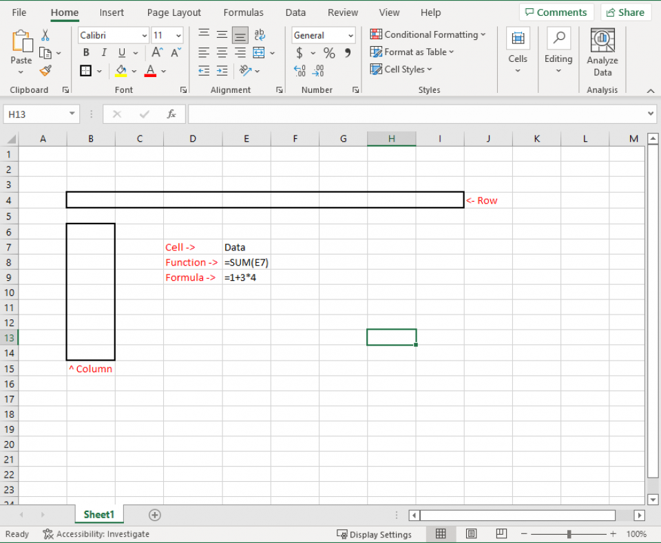
Excel Data Types

As a spreadsheet program, Excel focuses on storing data. Here are the data types that Excel frequently stores.

Text	Also called labels, text values identify data in a worksheet or store things like names and descriptions. Example: Hello, World!
Numbers	Numbers are used for calculations and can be formatted as currency, percentages, decimals, etc. Example: 1.12
Dates/Times	Dates and times track and calculate data over time. Example: 2022-02-02
Logical Values	Logical values are either true or false. Example: TRUE, FALSE
Arrays	Array formulas perform calculations on a range of cells simultaneously. Example: SUM(A1:A4)

Want To Master Excel? Take This Course.

Common Excel Functions

In Excel, a function is simply a preset formula or algorithm. They help parse information and display it for a variety of uses. Here are some of the most common Excel formulas in our Excel functions list cheat sheet.

SUM	Adds the values of a range of cells Example: SUM(A1:A4)
SUMIFS	Sums values that meet specific criteria. Example: SUMIFS(A1:A4,B1:B4,E1)
AVERAGE	Calculates the average values in a range of cells Example: AVERAGE(A1:A4)
COUNT	Counts the number of cells in a range that contains numbers Example: COUNT(A1:A4)
MIN	Finds the smallest value in a range of cells Example: MIN(A1:A4)
MAX	Finds the largest value in a range of cells Example: MAX(A1:A4)
TRIM	Removes all white space from the front and back of a cell. Example: TRIM(A1)
IF	Checks whether a condition is met and returns one value if true and another if false Example: IF(A1=‘Yes’, True, False)
CONCATENATE	Combines the values of multiple cells into a single cell. Example: CONCATENATE(A1, B1)
VALUE	Convert numbers that have been stored in text to integers. Example: VALUE(B1)
MIN	Finds the minimum value of a set. Example: MIN(A1:O1)
MAX	Finds the maximum value of a set. Example: MAX(A1:O1)
PROPER	Formats text with the correct capitalization; useful when importing data from other sources. Example: PROPER(A1)
CEILING	Round a number up to the first number of significance, e.g. 39.1 to either 39 or 40. Example: CEILING(A1,4)
FLOOR	Round a number down to the first number of significance, e.g. 39.12 to either 39.1 or 39. Example: FLOOR(A1,4)
LEN	Return the number of characters in a string, useful for data validation. Example: LEN(A1)
NOW	Get the current date and time. Note that it will return the time of the system you’re on. Example: NOW()
TODAY	Similar to now, but this just gives the date, rather than the date and time. You can also use DAY(), MONTH(), and YEAR(). Example: TODAY()

Advanced Excel Functions Cheat Sheet

These advanced Excel functions can be a little more difficult to use—but they’re sophisticated methods of processing and analyzing data.

VLOOKUP	Looks up a value in the leftmost column of a table and returns a corresponding value from another column Example: VLOOKUP(“Text”,A1:C4,2,FALSE)
INDEX	Performs a lookup based on a row and column number instead of a lookup value Example: INDEX(A1:A4,1,1)
HLOOKUP	Looks up a value in the top row of a table and returns a corresponding value from another row in the table Example: HLOOKUP(“Text”, A1:C4, 2)

Excel Shortcuts

Shortcuts are a great way to increase productivity. Once shortcuts become a habit, you’ll find even simpler tasks faster. Here are some of the most common keyboard shortcuts to help you work faster in Excel.

F2	Edit the active cell.
F5	Go to a specific cell in the worksheet.
CTRL + Arrow	Move to the edge of the worksheet’s data.
Shift + F11	Insert a new sheet.
Alt + =	Sum the cells.
Ctrl + Shift + “+”	Insert a new row/column.
Ctrl + “-”	Delete a row/column.
Ctrl + “*”	Select all cells with formulas.
Ctrl + ‘	Copy the value from above a cell.
Alt + Enter	Insert a line break in a cell.

Excel Commands

In addition to shortcuts, Excel has many built-in commands that can be accessed using shortcut keys or the ribbon. Here are some of the most common.

Paste Special	Opens the Paste Special dialog box, which allows you to choose how to paste data from the clipboard
Format Painter	Copies formatting from one cell and applies it to another cell or range of cells
Fill Handle	Allows you to quickly fill a range of cells with data that follows a pattern
AutoSum	Automatically calculates the sum of a range of selected cells
Sparklines	Creates small, graphical representations of data in a single cell

Excel Graphs

Not everything is readable in a series of columns and rows. When you need something human-readable, you need a graph. Excel offers several ways to create graphs and charts. Here are some of the most common.

Column Charts	Used to compare data points side-by-side.
Bar Charts	Used to compare data points side-by-side.
Line Charts	Used to show trends over time.
Pie Charts	Used to show percentages or proportions.
Scatter Plots	Used to show relationships between data points.

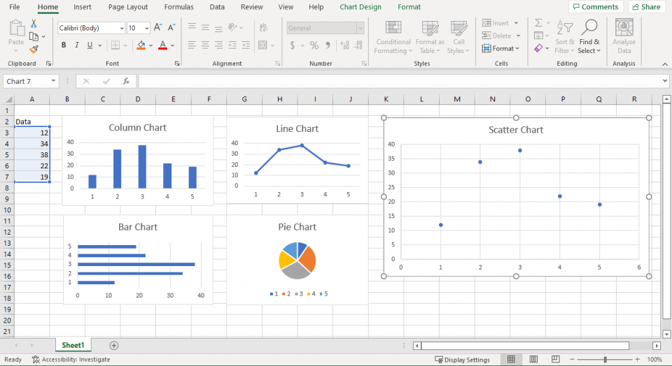
Tips and Tricks

Finally, here are a few tips and tricks to help you work faster in Excel.

Learn how to use keyboard shortcuts. Keyboard shortcuts can save you a lot of time working in Excel. Pressing CTRL+C will copy the selected cells, while CTRL+V will paste them.
Use the AutoFill feature when filling in similar values. The AutoFill feature in Excel is handy for filling in a data series. If you have a list of months, you can use AutoFill to fill in the days of the month automatically.
Use conditional formatting to increase the readability of your sheet. Conditional formatting allows you to highlight cells that meet specific criteria. You could use conditional formatting to highlight all cells that contain a value greater than 10.
Use data validation to ensure your sheet includes the right data types. You could use data validation to ensure cells only contain numbers—or only dates.
Memorize the most common and useful formulas. Formulas are one of the most powerful features in Excel, but they can take some time to learn.
Consider using macros. Macros are small programs that you can create to automate tasks in Excel. You could create a macro that automatically inserts the current date when you open a workbook or a macro that automatically saves and closes your files.
Get comfortable with pivot tables. Pivot tables are a great way to summarize large amounts of data and sort it.
Don’t be afraid of filters. Filters let you view only the data that you want to see. For example, you could use a filter only to view the data for a specific month.

Conclusion

A basic Excel cheat sheet or Excel commands cheat sheet can only do so much. It offers a quick alternative to building everything from scratch, and it helps users get started quickly. However, all spreadsheet users should learn the basics of Excel. Once you understand the capabilities, you should be able to look up things you need to know in the above Excel cheat sheet.

Frequently Asked Questions

1. How Do You Use the Cheat Sheet in Excel?

Use the above Excel function cheat sheet whenever you need to do something specific in Excel. You can review Excel cheat sheet formulas to refresh your memory or use CTRL+F to find a specific area of the Excel formula cheat sheet.

2. What are the 5 Functions in Excel?

Here’s a quick list of five basic Excel functions:

VLookup Formula
Text to Columns
Duplicate Removal
Pivot Tables
Concatenate Formula

3. What is the Fastest Way to Learn Excel Formulas?

Most formulas that you would need will pop up when you start typing in Excel. As long as you know what formulas are available in Excel, you should be able to look them up on this sheet.

4. What are the 7 Basic Excel Formulas?

The seven basic Excel formulas are SUM, AVERAGE, MIN, MAX, COUNT, COUNTA, and VLOOKUP. These are just a few of the many formulas available in Excel.

5. Where do you get Excel?

You can buy a copy of Excel from Microsoft as a stand-alone piece of software or get it as part of the Microsoft 365 suite of products. While Google offers a free alternative with their powerful sheets service, the original software has additional features professionals use every day.

People are also reading:

MySQL Create Database
Linux Cheat Sheet
GIT Cheat Sheet
CSS Cheat Sheet
PHP Cheat Sheet
HTML Cheat Sheet
SQL Cheat Sheet
Java Cheat Sheet
Bootstrap Cheat Sheet

Источник

Date and Time Functions

NOW and TODAY

DAY, MONTH, YEAR, and DATE

HOUR, MINUTE, SECOND, and TIME

DATEDIF and YEARFRAC

EDATE and EOMONTH

WORKDAY and NETWORKDAYS

WEEKDAY and WEEKNUM

Engineering

CONVERT

Information Functions

ISBLANK, ISERROR, ISNUMBER, and ISFORMULA

Logical Functions

AND, OR and NOT

IFERROR and IFNA

IF and IFS functions

Lookup and Reference Functions

VLOOKUP and HLOOKUP

INDEX and MATCH

LOOKUP

ROW and COLUMN

ROWS and COLUMNS

HYPERLINK

GETPIVOTDATA

CHOOSE

TRANSPOSE

OFFSET

INDIRECT

STATISTICAL Functions

COUNT and COUNTA

COUNTIF and COUNTIFS

SUM, SUMIF, SUMIFS

AVERAGE, AVERAGEIF, and AVERAGEIFS

MIN, MAX, LARGE, SMALL

MINIFS, MAXIFS

MODE

RANK

MATH Functions

ABS

RAND and RANDBETWEEN

ROUND, ROUNDUP, ROUNDDOWN, INT

MROUND, CEILING, FLOOR

MOD

SUMPRODUCT

SUBTOTAL

AGGREGATE

TEXT Functions

LEFT, RIGHT, MID

LEN

FIND, SEARCH

REPLACE, SUBSTITUTE

CODE, CHAR

TRIM, CLEAN

CONCAT, TEXTJOIN, CONCATENATE

EXACT

UPPER, LOWER, PROPER

TEXT

Dynamic Array functions

Quick navigation

List of Top 10 Commands in Excel

Table of contents

#1 VLOOKUP Function to Fetch Data

#2 IF Condition to Do Logical Test

#3 CONCATENATE Function to Combine Two or More Values

#4 Count Only Numerical Values

#5 Count All Values

#6 Count Based on Condition

#7 Count Number of Characters in the Cell

#8 Convert Negative Value to Positive Value

#9 Convert All Characters to UPPERCASE Values

#10 Find Maximum and Minimum Values

Things to Remember

Recommended Articles

Excel Advanced Concepts By J. Carlton Collins

Goal Seek

Scenarios

Database Queries

Download Excel Cheat Sheet PDF

Basic Terminology

The Anatomy of an Excel Sheet

Excel Advanced
Concepts
By J. Carlton Collins