
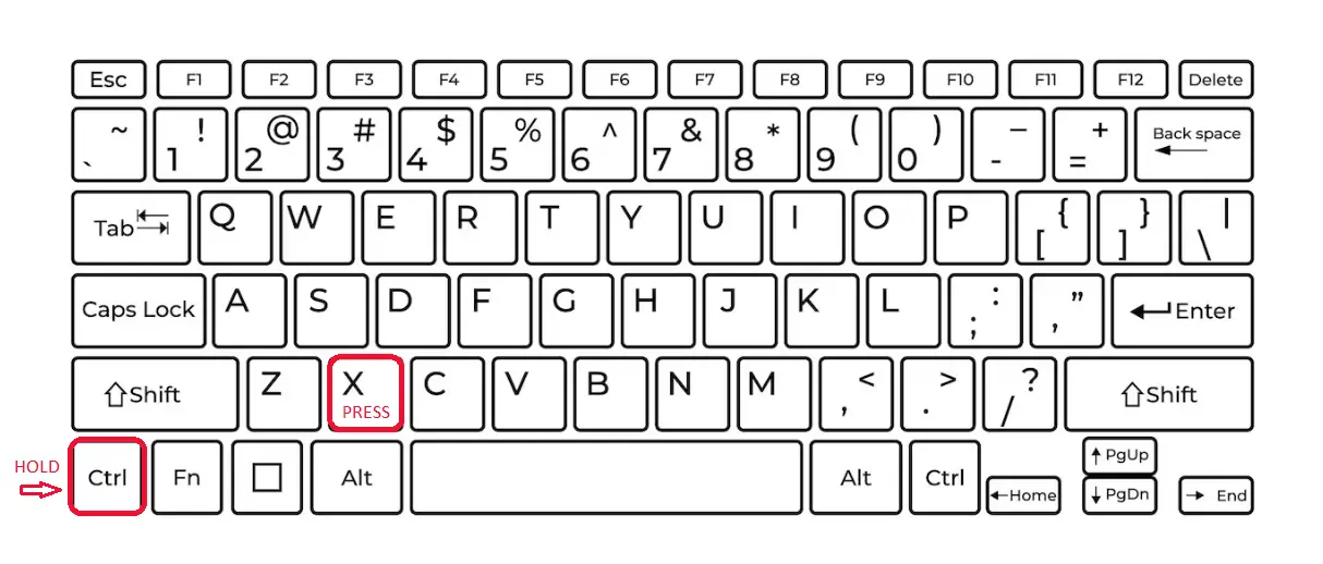
Cutting Data To cut data, select the cell or cells you want to cut and use the keyboard shortcut “Ctrl+X” (hold down the “Ctrl” key and the “X” key at the same time).
Contents
- 1 Can you clip cells in Excel?
- 2 How do I shorten a text string in Excel?
- 3 How do you clip data in Excel?
- 4 How do you isolate a cell in Excel?
- 5 How do I shorten text in a cell?
- 6 How do I cut text left in Excel?
- 7 How do I clip text in Excel 2020?
- 8 How do you make a long sentence in one cell in Excel?
- 9 How do I put a footer in Excel?
- 10 How do you select certain cells in Excel?
- 11 How do I return just the numbers in a cell?
- 12 How do you select a range of cells in Excel without dragging?
- 13 How do I remove 3 letters from a cell in Excel?
- 14 How do you trim the first character in Excel?
- 15 How do I remove a left and right character in Excel?
- 16 What is wrapped text in Excel?
- 17 Which option fits text in the cell?
- 18 How do I keep text in one cell in Excel without wrapping it?
- 19 How do I make a list in one cell in Excel?
- 20 How do I make multiple lines in one cell in Excel?
Can you clip cells in Excel?
In Excel, adjust the column to the required width, then enable word-warp on that column (which will cause all row heights to increase) and then finally select all rows and adjust row heights to the desired height. Voila!
How do I shorten a text string in Excel?
The formula is “=DIRECTION(Cell Name, Number of characters to display)” without the quotation marks. For example: =LEFT(A3, 6) displays the first six characters in cell A3. If the text in A3 says “Cats are better”, the truncated text will read “Cats a” in your selected cell.
How do you clip data in Excel?
Wrap text in a cell
- Select the cells.
- On the Home tab, click Wrap Text. The text in the selected cell wraps to fit the column width. When you change the column width, text wrapping adjusts automatically. Note: If all wrapped text is not visible, it might be because the row is set to a specific height.
How do you isolate a cell in Excel?
Place your mouse pointer on “Highlight Cell Rules” and review the list of options. Choose the one most appropriate for your purpose and click on it to open the rules dialog box. For example, select “equal to” to isolate a specific value or “duplicate values” to find duplicate data entries.
How do I shorten text in a cell?
How to truncate text in Excel – Excelchat
- Step 1: Prepare your data sheet.
- Step 2: Select cell/column where you want the truncated text string to appear.
- Step 3: Type the RIGHT or LEFT truncating formula in the target cell.
How do I cut text left in Excel?
Remove characters from left side of a cell
- =REPLACE(old_text, start_num, num_chars, new_text)
- =RIGHT(text,[num_chars])
- =LEN(text)
How do I clip text in Excel 2020?
On the Home tab, in the Alignment group, click Wrap Text. (On Excel for desktop, you can also select the cell, and then press Alt + H + W.) Notes: Data in the cell wraps to fit the column width, so if you change the column width, data wrapping adjusts automatically.
How do you make a long sentence in one cell in Excel?
Here is how I do it:
- Widen the column where the text is to be displayed to a reasonable width.
- Select the cell (or the entire column if you’re going to type lots of text throughout the column)
- Right-click on the selection.
- Choose “Format Cells”
- Click on the Alignment tab.
- Check the “Wrap text” box.
- Click OK.
On the Insert tab, in the Text group, click Header & Footer. Excel displays the worksheet in Page Layout view. To add or edit a header or footer, click the left, center, or right header or footer text box at the top or the bottom of the worksheet page (under Header, or above Footer). Type the new header or footer text.
How do you select certain cells in Excel?
Select one or more cells
- Click on a cell to select it. Or use the keyboard to navigate to it and select it.
- To select a range, select a cell, then with the left mouse button pressed, drag over the other cells.
- To select non-adjacent cells and cell ranges, hold Ctrl and select the cells.
How do I return just the numbers in a cell?
Extracting Numbers from the Right of a Text or Number String by Combining RIGHT, LEN, MIN & SEARCH Functions. Press Enter & then use Fill Handle to autofill the rest of the cells. MIN function is used to find the lowest digit or number from an array.
How do you select a range of cells in Excel without dragging?
Select a Large Range of Cells With the Shift Key
Click the first cell in the range you want to select. Scroll your sheet until you find the last cell in the range you want to select. Hold down your Shift key, and then click that cell. All the cells in the range are now selected.
How do I remove 3 letters from a cell in Excel?
1) In Number text, type the number of characters you want to remove from the strings, here I will remove 3 characters. 2) Check Specify option, then type the number which you want to remove string start from in beside textbox in Position section, here I will remove characters from third character.
How do you trim the first character in Excel?
1. Combine RIGHT and LEN to Remove the First Character from the Value. Using a combination of RIGHT and LEN is the most suitable way to remove the first character from a cell or from a text string. This formula simply skips the first character from the text provided and returns the rest of the characters.
How do I remove a left and right character in Excel?
In Excel 2013 and later versions, there is one more easy way to delete the first and last characters in Excel – the Flash Fill feature. In a cell adjacent to the first cell with the original data, type the desired result omitting the first or last character from the original string, and press Enter.
What is wrapped text in Excel?
“Wrapping text” means displaying the cell contents on multiple lines, rather than one long line. This will allow you to avoid the “truncated column” effect, make the text easier to read and better fit for printing. In addition, it will help you keep the column width consistent throughout the entire worksheet.
Which option fits text in the cell?
In “Table Tools” click the [Layout] tab > locate the “Cell Size” group and choose from of the following options: To fit the columns to the text (or page margins if cells are empty), click [AutoFit] > select “AutoFit Contents.”
How do I keep text in one cell in Excel without wrapping it?
If you want to hide the overflow text in a cell, such as A1 in this example, without having to type anything into the adjacent cells, right-click on the cell and select “Format Cells” from the popup menu. On the “Format Cells” dialog box, click the “Alignment” tab. Select “Fill” from the “Horizontal” drop-down list.
How do I make a list in one cell in Excel?
To have the entire list in a single Excel cell:
- Select the list in your word processor.
- Press Ctrl + C to copy it.
- Go to Excel > double-click your cell.
- Press Ctrl + V to paste the list. The list will appear in a single cell.
How do I make multiple lines in one cell in Excel?
You can put multiple lines in a cell with pressing Alt + Enter keys simultaneously while entering texts. Pressing the Alt + Enter keys simultaneously helps you separate texts with different lines in one cell. With this shortcut key, you can split the cell contents into multiple lines at any position as you need.
Working with Excel often involves rearranging the data in the worksheets.
And one common task many Excel users have to do is to cut the cell values from one cell and paste it to some other cell in the same worksheet or in another worksheet/workbook.
While this is a basic operation that most Excel users are often aware of, in case you’re a beginner, I’ll show you everything you need to know about how to cut a cell value in Excel.
Keyboard Shortcut to Cut Cell Value (or Range of Cells)
Let’s first start with the simplest and the most common way of cutting a cell value in Excel – a keyboard shortcut.
Control + X
Below are the steps to use the above keyboard shortcut to cut cell values in Excel:
- Select the cell or range of cells that you want to cut
- Hold the Control key on your keyboard (use the Command key instead of the Control key if you’re using a Mac)
- Press the X key. You will see dancing ants (a dashed outline) around the selection

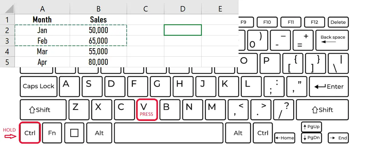
- Select say where you want to copy the cell/range that you cut
- Use the keyboard shortcut Control + V to paste the cut cells (hold the Control key and then press the V key)
Also read: 200+ Excel Keyboard Shortcuts – 10x Your Productivity
Cut Cells Using Mouse Drag and Drop
If you perform using your mouse over using the keyboard shortcuts, you can easily do that as well.
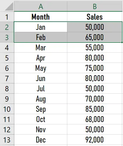
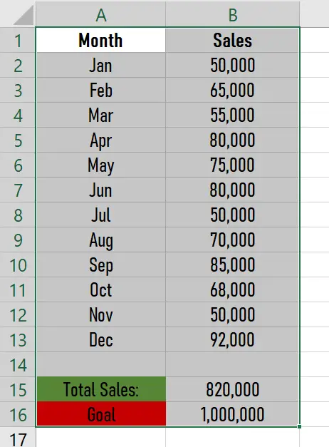
Below I have a dataset where I want to cut to the cells in column A and paste these in column C.

Below are the steps to do this using mouse drag and drop:
- Select the range of cells that you want to cut
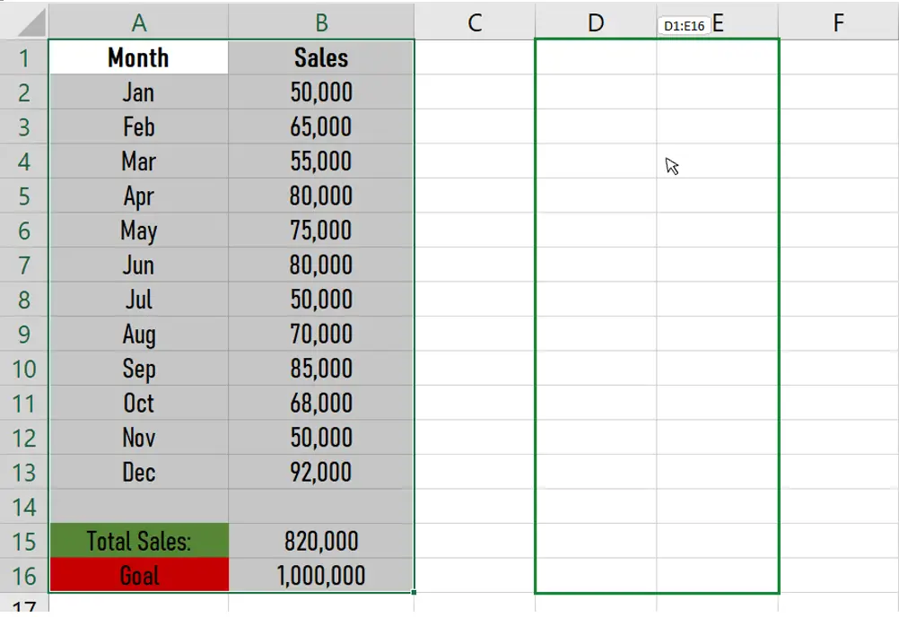
- Place the cursor at the edge of the selection. You will notice that the cursor changes and shows a four-arrow icon (as shown below)

- Press the left mouse key and hold it
- Drag the cursor to the position where you want these cells to be pasted
- Leave the mouse key
The above steps would cut the selected cells and then paste them where you have the cursor.
While you may think that these are a lot of steps compared to a keyboard shortcut, in my experience, this method is equally fast if you want to cut and paste cells in a nearby area.
Where this fails is when you want to cut the cells and paste them in some other worksheet or some other workbooks (as this only works in the same worksheet).
Also read: Boost Your Productivity with Excel Mouse Double Click Tricks
Cut Partial Cell Value Using Keyboard Shortcut
Sometimes, you may want to cut only a part of the content in a cell and not the entire cell itself.
In such a scenario, the only way to do this is to get into the edit mode in the cell, manually select the content that you want to cut, use the keyboard shortcut to cut that content, and then paste it wherever you want.
Below I have the text “It’s a Wonderful Day” in cell A1, And I want to only cut the text “Wonderful Day”.

Here are the steps to do this:
- Select the cells that have the content that you want to cut (cell A1 in our example)
- Double-click on the cell or press the F2 key to get into the edit mode (you’ll see the cursor blinking in the cell when you are in the edit mode)
- Use your mouse to drag the cursor and select the cell that you want to cut

- Use the keyboard shortcut Control + X to cut the text
- Select the cell where you want to paste this text
- Paste the copied content by using the keyboard shortcut Control V
While it’s possible for you to copy multiple cells and cut and paste them at the same time, when you want to cut partial text from a cell, you need to do it one cell at a time.
Note: You can also select the partial text by selecting the cell and then copying the text from the Formula Bar
In this tutorial, I showed you a simple keyboard shortcut that you can use to quickly cut and paste cell values in Excel.
I also covered how you can use the mouse drag-and-drop technique to do the same thing without using a keyboard shortcut. And I also covered how you can cut partial text from a cell in excel.
I hope you found this Excel tutorial useful.
Other Excel tutorials you may also like:
- Save As Shortcuts in Excel (Quick and Easy)
- Copy and Paste Multiple Cells in Excel (Adjacent & Non-Adjacent)
- How to Copy and Paste Columns in Excel? 3 Easy Ways!
- How to Copy and Paste Formulas in Excel without Changing Cell References
- Working with Cells and Ranges in Excel VBA (Select, Copy, Move, Edit)
- How to Start a New Line in Excel Cell (Keyboard Shortcut + Formula)
Move or copy cells and cell contents
Use Cut, Copy, and Paste to move or copy cell contents. Or copy specific contents or attributes from the cells. For example, copy the resulting value of a formula without copying the formula, or copy only the formula.
When you move or copy a cell, Excel moves or copies the cell, including formulas and their resulting values, cell formats, and comments.
You can move cells in Excel by drag and dropping or using the Cut and Paste commands.

Move cells by drag and dropping
-
Select the cells or range of cells that you want to move or copy.
-
Point to the border of the selection.
-
When the pointer becomes a move pointer
 , drag the cell or range of cells to another location.
 , drag the cell or range of cells to another location.
Move cells by using Cut and Paste
-
Select a cell or a cell range.
-
Select Home > Cut
or press Ctrl + X. -
Select a cell where you want to move the data.
-
Select Home > Paste
or press Ctrl + V.
 or press Ctrl + X.
 or press Ctrl + V.
Copy cells by using Copy and Paste
-
Select the cell or range of cells.
-
Select Copy or press Ctrl + C.
-
Select Paste or press Ctrl + V.
Need more help?
You can always ask an expert in the Excel Tech Community or get support in the Answers community.
See Also
Move or copy cells, rows, and columns
Need more help?
If you’re working with data in Excel that you’ve imported from other sources, sometimes you have to work with data that isn’t in a format that you want. This is especially true with comma-delimited text that comes into single cells.
The only way to deal with that data is to split a cell in Excel. There are different ways to do this, depending on the format of the data.

In this article you’ll learn how to split a cell, how to roll that out to an entire column, and when you should choose each option.
Convert Text To Columns
One of the most common methods to split a cell in Excel is using the Text to Columns tool. This lets you split an entire column of cells using whatever rules you like.
The feature also includes an easy-to-use wizard, which is why most people prefer using it. It also handles any text format, whether the separating text is a space, a tab, or a comma.
Let’s look at an example of how to use the Text to Columns feature in Excel.
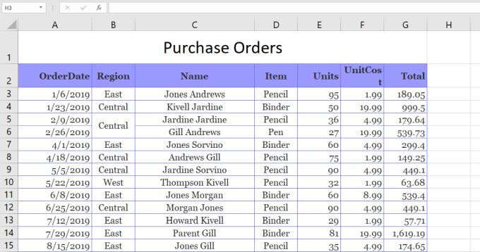
In this example, we want to split the Name column into two cells, the first name and the last name of the salesperson.
To do this:
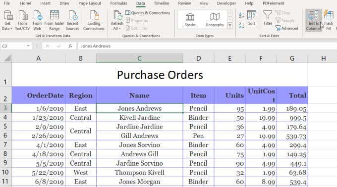
1. Select the Data menu. Then select Text to Columns in the Data Tools group on the ribbon.
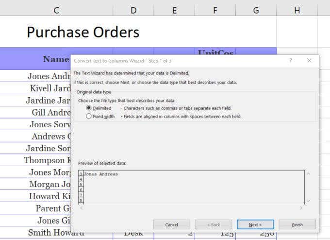
2. This will open a three-step wizard. In the first window, make sure Delimited is selected and select Next.
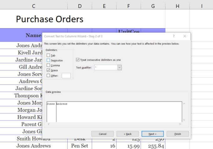
3. On the next Wizard window, deselect Tab and make sure Space is selected. Select Next to continue.
4. On the next window, select the Destination field. Then, in the spreadsheet, select the cell where you want the first name to go. This will update the cell in the Destination field to where you’ve selected.
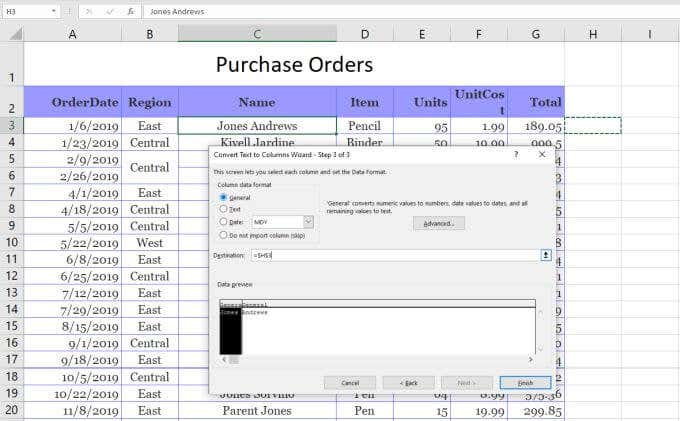
5. Now, select Finish to complete the Wizard.
You’ll see that the single cell that contained both the first name and last name has been split into two cells that contain each one individually.
Note: The process above works because the data to split in the cell had a space separating the text. This text-to-column feature can also handle splitting a cell in Excel if the text is separated by a tab, semicolon, comma, or any other character you specify.
Use Excel Text Functions
Another way to split a cell in Excel is by using different text functions. Text functions let you extract pieces of a cell that you can output into another cell.
Text functions in Excel include:
- Left(): Extract a number of characters from the left side of the text
- Right(): Extract a number of characters from the right side of the text
- Mid(): Extract a number of characters from the middle of a string
- Find(): Find a substring inside of another string
- Len(): Return the total number of characters in a string of text
To split cells, you may not need to use all of these functions. However, there are multiple ways you can use these to accomplish the same thing.
For example, you can use the Left and Find function to extract the first name. The Find function helps because it can tell you where the delimiting character is. In this case, it’s a space.
So the function would look like this:
=LEFT(C3,FIND(” “,C3))
When you press enter after typing this function, you’ll see that the first name is extracted from the string in cell C3.
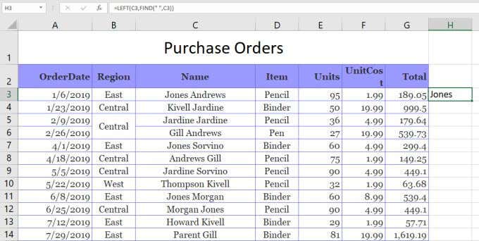
This works, because the Left function needs the number of characters to extract. Since the space character is positioned at the end of the first name, you can use the FIND function to find the space, which returns the number of characters you need to get the first name.
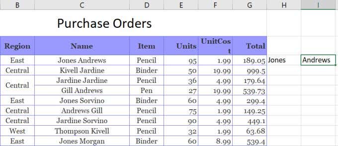
You can extract the last name either using either the Right function or the Mid function.
To use the Right function:
=RIGHT(C3,LEN(C3)-FIND(” “,C3))
This will extract the last name by finding the position of the space, then subtracting that from the length of the total string. This gives the Right function the number of characters it needs to extract the last name.
Technically, you could do the same thing as the Right function using the Mid function, like this:
=MID(C3,FIND(” “,C3),LEN(C3)-FIND(” “,C3))
In this case the Find function gives the Mid function the starting point, and the Len combined with Find provides the number of characters to extract. This will also return the last name.
Using Excel text functions to split a cell in Excel works as well as the Text-To-Column solution, but it also lets you fill the entire column beneath those results using the same functions.
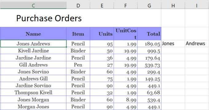
Split Cell in Excel Using Flash Fill
The last option to split a cell in Excel is using the Flash Fill feature. This requires that the cells you’re splitting the original one into are right beside it.
If this is the case, all you have to do is type the part of the original cell that you want to split out. Then drag the lower right corner of the cell down to fill the cell beneath it. When you do this, you’ll see a small cell fill icon appear with a small plus sign next to it.
Select this icon and you’ll see a menu pop-up. Select Flash Fill in this menu.
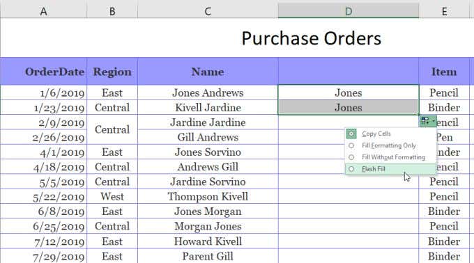
When you do this, you’ll see that the Flash Fill feature automatically detects why you typed what you typed, and will repeat the process in the next cell. It’ll do this by detecting and filling in the first name in the original cell to the left.
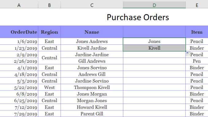
You can actually do this same procedure when you fill the entire column. Select the same icon and select Flash Fill. It’ll fill the entire column with the correct first name from the cells to the left.
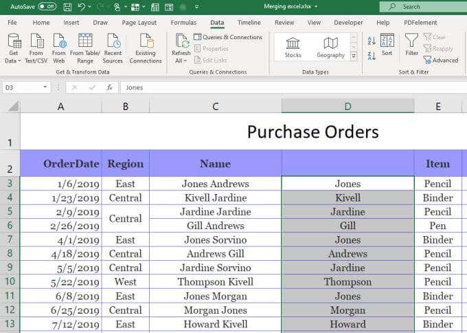
You can then copy this entire column and paste it into another column, then repeat this same process to extract the last names. Finally, copy and paste that entire column where you want it to go in the spreadsheet. Then delete the original column you used to perform the Flash Fill process.
Splitting Cells in Excel
As you can see there are a few ways to accomplish the same thing. How you split a cell in Excel boils down to where you want the final result to go and what you plan to do with it. Any options works, so choose the one that makes the most sense for your situation and use it.
In this tutorial, we will learn the shortcut for how to cut a cell value in Excel. We can guarantee you that this will make your work in Excel easier.
Working with Excel is easy when you know its functions and basic operations. If you are a beginner, worry no more, as we will teach you everything you need to know in Excel. All you have to do is visit our website and see tons of Excel tutorials.
Without further ado, let’s get to our tutorial on how to cut a cell value in Excel shortly before we get too far.
Time needed: 1 minute.
Here’s a step-by-step guide on how to cut a cell value in Excel using a keyboard shortcut.
- Select the cell or range of cells.
The first thing you do is select the cell or range of cells that you want to cut.

- Hold the CTRL key, then press the X key.
The next thing you do is hold the control key, then press the X key on your keyboard.
Note: After holding the control key and pressing the X key, you’ll see a moving line around your selection or a dashed outline.

- Select a cell, then paste the cell or cell range you cut.
After the second step, select a cell where you want to move or paste the cell or cell range you cut. Then, hold the control key and press the V key.
Note: If you want to move the cells that you cut to another worksheet, you just have to add a worksheet and then paste it there. In the same process, you select a cell on that sheet and then paste it.
Cut cells using the mouse
Wondering if cutting a cell with a mouse is possible? The answer is yes since you can accomplish that very quickly. All you have to do is drag and drop.
The following are steps to cut cells using the mouse by dragging and dropping.
Step 1: Select or emphasize the cell or a set of cells that you would like to remove.
Step 2: Put the cursor at the selection’s edge.
Note: When you place your cursor there, the arrow or cursor changes into a four-arrow icon.

Step 3: Press and hold the left mouse key.

Step 4: Drag the selected cells to the cells where you want them to move.
Conclusion
In conclusion, this tutorial is essential for making Excel work uncomplicated and more productive. Learning keyboard shortcuts is crucial since they speed up our work, not just simplify it.
I believe that we have accomplished this tutorial. I hope you’ve learned something from this. If you have any questions or suggestions, please leave a comment below, and for more educational content, visit our website.
Thank you for reading!