Custom lists in excel - Word и Excel - помощь в работе с программами

Create or delete a custom list for sorting and filling data

Excel for Microsoft 365 Excel 2021 Excel 2019 Excel 2016 Excel 2013 Excel 2010 Excel 2007 More…Less

Use a custom list to sort or fill in a user-defined order. Excel provides day-of-the-week and month-of-the year built-in lists, but you can also create your own custom list.

To understand custom lists, it is helpful to see how they work and how they are stored on a computer.

Comparing built-in and custom lists

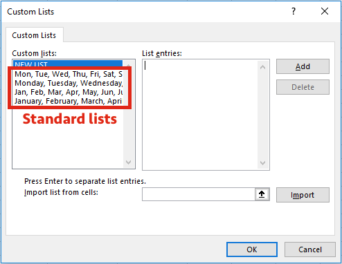
Excel provides the following built-in, day-of-the-week, and month-of-the year custom lists.

Built-in lists
Sun, Mon, Tue, Wed, Thu, Fri, Sat
Sunday, Monday, Tuesday, Wednesday, Thursday, Friday, Saturday
Jan, Feb, Mar, Apr, May, Jun, Jul, Aug, Sep, Oct, Nov, Dec
January, February, March, April, May, June, July, August, September, October, November, December

Note: You cannot edit or delete a built-in list.

You can also create your own custom list, and use them to sort or fill. For example, if you want to sort or fill by the following lists, you’ll need to create a custom list, since there is no natural order.

Custom lists
High, Medium, Low
Large, Medium, and Small
North, South, East, and West
Senior Sales Manager, Regional Sales Manager, Department Sales Manager, and Sales Representative

A custom list can correspond to a cell range, or you can enter the list in the Custom Lists dialog box.

Note: A custom list can only contain text or text that is mixed with numbers. For a custom list that contains numbers only, such as 0 through 100, you must first create a list of numbers that is formatted as text.

There are two ways to create a custom list. If your custom list is short, you can enter the values directly in the popup window. If your custom list is long, you can import it from a range of cells.

Enter values directly

Follow these steps to create a custom list by entering values:

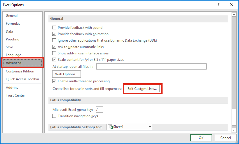
For Excel 2010 and later, click File > Options > Advanced > General > Edit Custom Lists.
For Excel 2007, click the Microsoft Office Button > Excel Options > Popular >Top options for working with Excel > Edit Custom Lists.
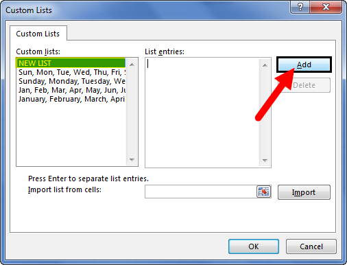
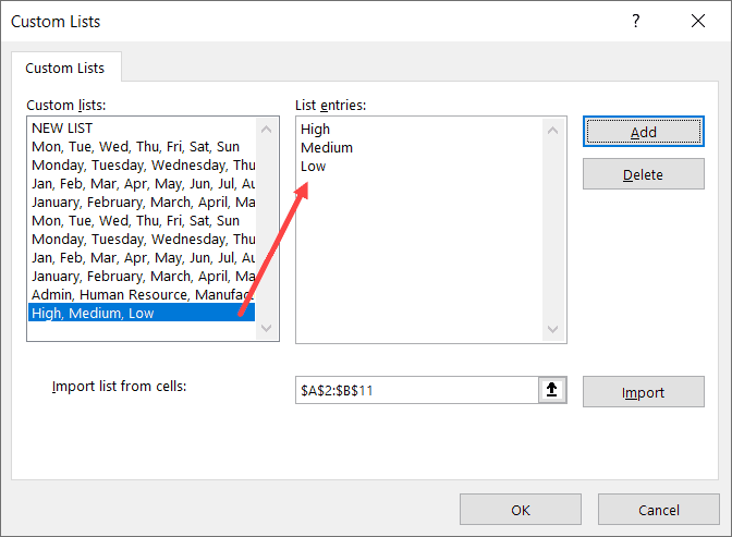
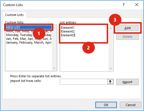
In the Custom Lists box, click NEW LIST, and then type the entries in the List entries box, beginning with the first entry.

Press the Enter key after each entry.
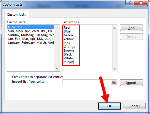
When the list is complete, click Add.

The items in the list that you have chosen will appear in the Custom lists panel.
Click OK twice.

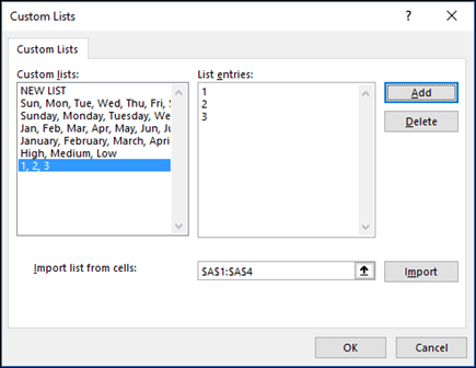
Create a custom list from a cell range

Follow these steps:

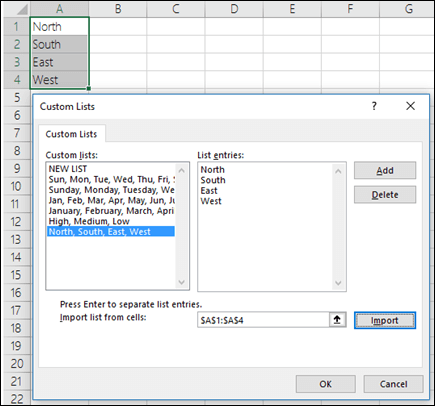
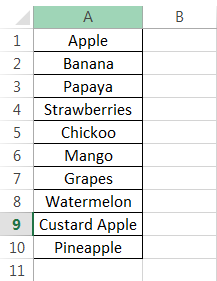
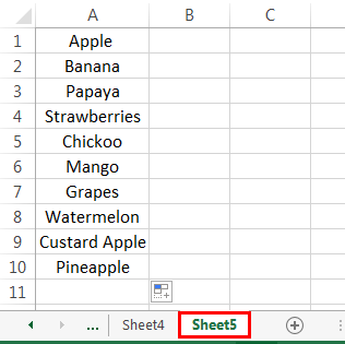
In a range of cells, enter the values that you want to sort or fill by, in the order that you want them, from top to bottom. Select the range of cells you just entered, and follow the previous instructions for displaying the Edit Custom Lists popup window.
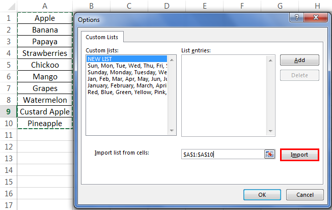
In the Custom Lists popup window, verify that the cell reference of the list of items that you have chosen appears in the Import list from cells field, and then click Import.
The items in the list that you have chosen will appear in the Custom Lists panel.
Click OK twice.

Note: You can only create a custom list according to values, such as text, numbers, dates or times. You cannot create a custom list for formats such as cell color, font color, or an icon.

Follow these steps:

Follow the previous instructions for displaying the Edit Custom Lists dialog.
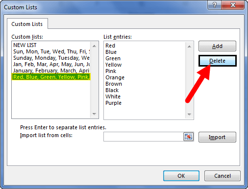
In the Custom Lists box, choose the list that you want to delete, and then click Delete.

Once you create a custom list, it is added to your computer registry, so that it is available for use in other workbooks. If you use a custom list when sorting data, it is also saved with the workbook, so that it can be used on other computers, including servers where your workbook might be published to Excel Services and you want to rely on the custom list for a sort.

However, if you open the workbook on another computer or server, you do not see the custom list that is stored in the workbook file in the Custom Lists popup window that is available from Excel Options, only from the Order column of the Sort dialog box. The custom list that is stored in the workbook file is also not immediately available for the Fill command.

If you prefer, add the custom list that is stored in the workbook file to the registry of the other computer or server and make it available from the Custom Lists popup window in Excel Options. From the Sort popup window, in the Order column, select Custom Lists to display the Custom Lists popup window, then select the custom list, and then click Add.

Need more help?

You can always ask an expert in the Excel Tech Community or get support in the Answers community.

Need more help?

Want more options?

Explore subscription benefits, browse training courses, learn how to secure your device, and more.

Communities help you ask and answer questions, give feedback, and hear from experts with rich knowledge.

Источник

Custom lists in Excel are used to sort data based on the user’s choice. It is especially useful when you need to perform multiple tasks on the same data on a repetitive basis. For example, under normal sort, Excel provides general options to sort from A to Z or high or low, but with a custom list, you can sort the data as per your desire.

How to Create a Custom List in Excel?
- Example #1 – Custom List Created Manually in Excel
- Example #2 – Create List in Different Sheet
- Things to Remember
- Recommended Articles

How to Create a Custom List in Excel?

Let us learn how to create a custom list in Excel using practical examples –

Example #1 – Custom List Created Manually in Excel

Let us follow the below steps:

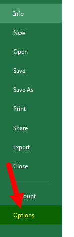
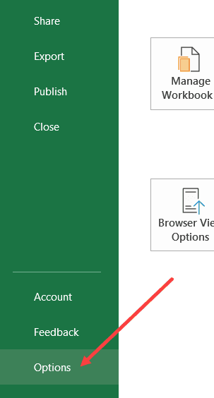
First, we must open Excel. Then, go to “File” and select “Options.”
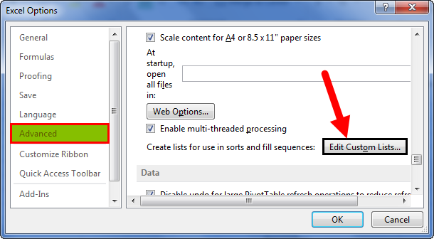
Then, choose “Advanced” and click on “Edit Custom Lists.”
Then, we need to click on “New List,” then click on “Add.”
Next, we must write details in the “List Entries” box. Then, press “Enter” after writing each entry. Finally, click “OK” after writing all the details.
Click on the “OK” option.
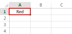
Then, we need to go to the Excel file. And type the first name only from the entry list.
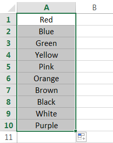
Then, drag from the first entry done in the Excel file.
As a result, details are now automatically updated, without the need to type manually in an Excel file. It is an example of a custom list created manually by a user in Excel.
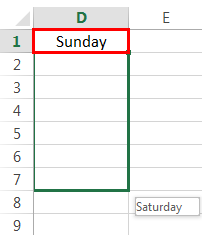
Days of the week need not be created manually in the Excel custom list, even if the first day of the week is inserted.

Then the first entry cell is dragged, and other weekdays get auto-populated. This list already exists in Excel and cannot be deleted by the user.

Months of the year also exist in Excel. Therefore, there is no need to manually create a list for days of the month in Excel.
Then, we must write the month name in a cell and drag that cell. Consequently, the month’s name gets automatically populated.
A manually created list by the user is now visible in the Excel custom lists. In addition, we can click the Delete to delete the manually made list.
We can create the list either horizontally or vertically.

Example #2 – Create List in Different Sheet

We can also create lists on a different sheet.

Step 1 – We must first enter the details in the new sheet.

Step 2 – Then, we need to go to the new list. Click on “Add,” then click on “Arrow.”

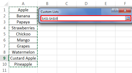
Step 3 – Custom list in Excel gets populated. Now, we must select newly entered details. Then, the dollar and semicolon sign automatically gets created. There is no need to make these signs manually.

Step 4 – Next, click on “Import” and click “OK” twice.

Step 5 – Go to another sheet. Again, we must type the first name from the entry list and drag the cell from the first entry.

Instead, we can see this list on another sheet.

The user does not enter a comma. Instead, a comma gets automatically created in the custom lists dialog.

Note: The above examples were done in Excel 2013.

Go to File---options---advanced—edit custom list and follow the same steps as above for doing in Excel 2007.

TOOLS-- OPTIONS-- CUSTOM LIST and follow same steps as above for doing in Excel 2003.

Things to Remember

Avoid creating a list that already exists. For example, days of the week, months in a year.
Remember the first entry is made while preparing the list.
Do not keep lengthy sentences on the list. A custom list in Excel helps in data collection and creating reports.
Entries in a list can be either changed or deleted as per user preference.

How to Create Custom Lists in Excel

By default, Excel already has some pre-fed custom lists that you can use to save time.

For example, if you enter ‘Mon’ in one cell ‘Tue’ in an adjacent cell, you can use the fill handle to fill the rest of the days. In case you extend the selection, keep on dragging and it will repeat and give you the day’s name again.

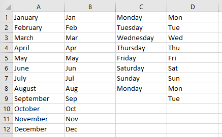
Below are the custom lists that are already in-built in Excel. As you can see, these are mostly days and month names as these are fixed and will not change.

Now, suppose you want to create a list of departments that you often need in Excel, you can create a custom list for it. This way, the next time you need to get all the departments name in one place, you don’t need to rummage through old files. All you need to do is type the first two in the list and drag.

Below are the steps to create your own Custom List in Excel:

Click the File tab
Click on Options. This will open the ‘Excel Options‘ dialog box
Click on the Advanced option in the left-pane
In the General option, click on the ‘Edit Custom Lists’ button (you may have to scroll down to get to this option)
In the Custom Lists dialog box, import the list by selecting the range of cells that have the list. Alternatively, you can also enter the name manually in the List Entries box (separated by comma or each name in a new line)
Click on Add

As soon as you click on Add, you would notice that your list now becomes a part of the Custom Lists.

In case you have a large list that you want to add to Excel, you can also use the Import option in the dialog box.

Pro tip: You can also create a named range and use that named range to create the custom list. To do this, enter the name of the named range in the ‘Import list from cells’ field and click OK. The benefit of this is that you can change or expand the named range and it will automatically get adjusted as the custom list

Now that you have the list in Excel backend, you can use it just like you use numbers or month names with Autofill (as shown below).

While it’s great to be able to quickly get these custom lits names in Excel by doing a simple drag and drop, there is something even more awesome that you can do with custom lists (that’s what the next section is about).

Create Your Own Sorting Criteria Using Custom Lists

One great thing about custom lists is that you can use it to create your own sorting criteria. For example, suppose you have a dataset as shown below and you want to sort this based on High, Medium, and Low.

You can’t do this!

If you sort alphabetically, it would screw the alphabetical order (it will give you High, Low, and Medium and not High, Medium, and Low).

This is where Custom Lists really shine.

You can create your own list of items and then use these to sort the data. This way, you will get all the High values together at the top followed by the medium and low values.

The first step is to create a custom list (High, Medium, Low) using the steps shown in the previous section (‘How to Create Custom Lists in Excel‘).

Once you have the custom list created, you can use the below steps to sort based on it:

Select the entire dataset (including the headers)
Click the Data tab
In the Sort and Filter group, click on the Sort icon. This will open the Sort dialog box
In the Sort dialog box, make the following selections:
- Sort by Column: Priority
- Sort On: Cell Values
- Order: Custom Lists. When the dialog box opens, select the sorting criteria you want to use and then click on OK.
Click OK

The above steps would instantly sort the data using the list you created and used as criteria while sorting (High, Medium, Low in this example).

Note that you don’t necessarily need to create the custom list first to use it in sorting. You can use the above steps and in Step 4 when the dialog box opens, you can create a list right there in that dialog box.

Some Examples Where you can Use Custom Lists

Below are some of the cases where creating and using custom lists can save you time:

If you have a list that you need to enter manually (or copy-paste from some other source), you can create a custom list and use that instead. For example, this could be department names in your organization, or product names or regions/countries.
If you’re a teacher, you can create a list of your student names. That way, when you are grading them the next time, you don’t need to worry about entering the student names manually or copy-pasting it from some other sheet. This also ensures that there are fewer chances of errors.
When you need to sort data based on criteria that are not in-built in Excel. As covered in the previous section, you can use your own sorting criteria by making a custom list in Excel.

So this is all that you need to know about Creating Custom Lists in Excel.

I hope you found this useful.

You may also like the following Excel tutorials:

How to Sort by the Last Name in Excel
How to SORT in Excel (by Rows, Columns, Colors, Dates, & Numbers)
How to Sort By Color in Excel
How to Sort Worksheets in Excel
Automatically Sort Data in Alphabetical Order using Formula

Источник

Do you ever find yourself typing out the same standard lists over and over again, such as lists of products, cost centers, projects or companies? I do. It is essential these lists don’t exclude any items and are presented in the same order each time. Lists of 4 or 5 things are easy to remember, but my brain starts to struggle when there are 6 or more. Plus, the time it takes to type those lists is a big waste of time. So, I decided to stop remembering and let Excel do the remembering for me.

AutoFill Lists

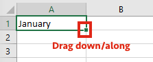
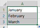
Excel loves to remember lists, it even has some built-in as standard; the months of the year and the days of the week. If you type ‘January’ into a cell, then drag that cell down/across Excel enters ‘February’ automatically, then ‘March’ and so on.

You could equally try the days of the week. ‘Monday’ will drag to become ‘Tuesday’, ‘Wednesday’ etc.

Excel doesn’t care where the list starts, type ‘Friday’ and it will populate the following days correctly. It also includes abbreviations, so ‘Jan’ for ‘January’ and ‘Mon’ for ‘Monday’. Try them, they will all populate correctly.

You can type the case of the first item as you need and the others will be the same. So, if you type it in upper case all the following items will be in uppercase.

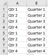
There are a few hidden lists too, such as the quarters of the year.

But you are not limited to the standard lists, Excel lets you can create your own.

From the Ribbon, Click: File -> Options.

In the Excel Options window, scroll all the way down to the bottom, until you reach the General section. Click the Edit Custom Lists . . . button.

The Custom Lists window will open. You can now see where the lists for the months of the year or days of the week are stored.

To create your own lists, there are two methods of data entry:

Method 1 – Manual Entry

Click on NEW LIST in the Custom lists box [1].

Start typing the list in the List entries box [2].

Once complete click Add [3].

That’s it, your list is now ready to be used in a worksheet.

Method 2 – Import

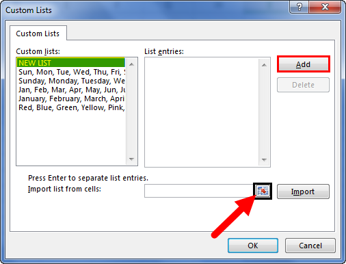
Click on NEW LIST in the Custom lists box [1].

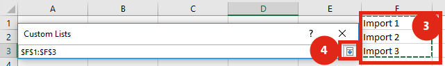
Click on the Range Input icon from the Import list from cells box [2].

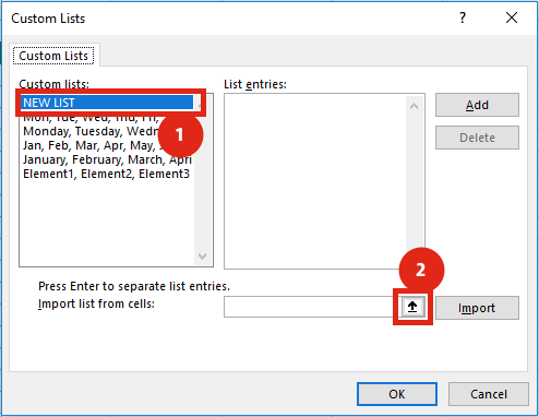
Select the location of the list [3], then click on the icon to return [4].

Back in the Custom Lists window, click Import [5].

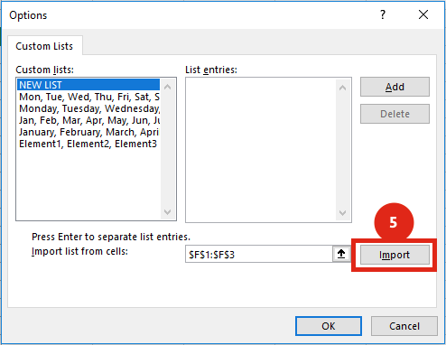
That’s it, your list is now ready to be used in a worksheet.

Using your new Custom List

Click on a cell and type in the first item in your new Custom List, drag it down or along, just as you did for the months and days. The cells will populate with your new Custom List.

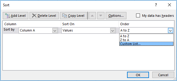
You can also sort by your Custom Lists too. In the Sort window select Custom List… from the Order drop-down box – simple.

The Custom List only exists on your computer, it will not be available for others to use unless they create the same Custom List on their own computer.

Editing a Custom List

To edit a list, click on it in the Custom Lists window and change it. Click Add to confirm the change.

Any Custom List which has been used on a worksheet is not linked in any way to the original list. i.e. If you change the elements in the Custom List it will not change any lists already existing on your worksheets.

Managing Custom Lists with VBA

If you wanted to manage Custom Lists (creating, deleting, checking for existence etc.) then check out my VBA Code Snippets.

About the author

Hey, I’m Mark, and I run Excel Off The Grid.

My parents tell me that at the age of 7 I declared I was going to become a qualified accountant. I was either psychic or had no imagination, as that is exactly what happened. However, it wasn’t until I was 35 that my journey really began.

In 2015, I started a new job, for which I was regularly working after 10pm. As a result, I rarely saw my children during the week. So, I started searching for the secrets to automating Excel. I discovered that by building a small number of simple tools, I could combine them together in different ways to automate nearly all my regular tasks. This meant I could work less hours (and I got pay raises!). Today, I teach these techniques to other professionals in our training program so they too can spend less time at work (and more time with their children and doing the things they love).

Do you need help adapting this post to your needs?

I’m guessing the examples in this post don’t exactly match your situation. We all use Excel differently, so it’s impossible to write a post that will meet everybody’s needs. By taking the time to understand the techniques and principles in this post (and elsewhere on this site), you should be able to adapt it to your needs.

But, if you’re still struggling you should:

Read other blogs, or watch YouTube videos on the same topic. You will benefit much more by discovering your own solutions.
Ask the ‘Excel Ninja’ in your office. It’s amazing what things other people know.
Ask a question in a forum like Mr Excel, or the Microsoft Answers Community. Remember, the people on these forums are generally giving their time for free. So take care to craft your question, make sure it’s clear and concise. List all the things you’ve tried, and provide screenshots, code segments and example workbooks.
Use Excel Rescue, who are my consultancy partner. They help by providing solutions to smaller Excel problems.

What next?
Don’t go yet, there is plenty more to learn on Excel Off The Grid. Check out the latest posts:

Источник

If you create a custom list in Excel, you can easily fill a range with your own list of departments, clients, cities, credit card numbers, etc. This can save time and reduce errors.

First, we will look at an example of a built-in list.

1. Type Sun into cell B2.