
Change the format of a cell
You can apply formatting to an entire cell and to the data inside a cell—or a group of cells. One way to think of this is the cells are the frame of a picture and the picture inside the frame is the data.

Formal Cells
-
Select the cells.
-
Go to the ribbon to select changes as Bold, Font Color, or Font Size.
Apply Excel Styles
-
Select the cells.
-
Select Home > Cell Style and select a style.
Modify an Excel Style
-
Select the cells with the Excel Style.
-
Right-click the applied style in Home > Cell Styles.
-
Select Modify > Format to change what you want.
Need more help?
You can always ask an expert in the Excel Tech Community or get support in the Answers community.
See Also
Format text in cells
Format numbers
Format a date the way you want
Need more help?
При необходимости Вы можете легко добавить к стандартным числовым форматам Excel свои собственные. Для этого выделите ячейки, к которым надо применить пользовательский формат, щелкните по ним правой кнопкой мыши и выберите в контекстном меню команду Формат ячеек (Format Cells) — вкладка Число (Number), далее — Все форматы (Custom):

В появившееся справа поле Тип: введите маску нужного вам формата из последнего столбца этой таблицы:

Как это работает…
На самом деле все очень просто. Как Вы уже, наверное, заметили, Excel использует несколько спецсимволов в масках форматов:
- 0 (ноль) — одно обязательное знакоместо (разряд), т.е. это место в маске формата будет заполнено цифрой из числа, которое пользователь введет в ячейку. Если для этого знакоместа нет числа, то будет выведен ноль. Например, если к числу 12 применить маску 0000, то получится 0012, а если к числу 1,3456 применить маску 0,00 — получится 1,35.
- # (решетка) — одно необязательное знакоместо — примерно то же самое, что и ноль, но если для знакоместа нет числа, то ничего не выводится
- (пробел) — используется как разделитель групп разрядов по три между тысячами, миллионами, миллиардами и т.д.
- [ ] — в квадратных скобках перед маской формата можно указать цвет шрифта. Разрешено использовать следующие цвета: черный, белый, красный, синий, зеленый, жёлтый, голубой.
Плюс пара простых правил:
- Любой пользовательский текст (кг, чел, шт и тому подобные) или символы (в том числе и пробелы) — надо обязательно заключать в кавычки.
- Можно указать несколько (до 4-х) разных масок форматов через точку с запятой. Тогда первая из масок будет применяться к ячейке, если число в ней положительное, вторая — если отрицательное, третья — если содержимое ячейки равно нулю и четвертая — если в ячейке не число, а текст (см. выше пример с температурой).
Ссылки по теме
- Как скрыть содержимое ячейки с помощью пользовательского формата
Learning how to customise a cell format in Excel allows you to not only format your data the way you want, but in some instances it can save you time.
Before we dive in you need to know that despite how the text appears after you’ve set your custom cell format, the underlying value is unchanged for the purpose of formulas and calculations.
How to enter an Excel custom cell format
Select the cell/s you want to format then open the Format Cells window.
- The quick way just press CTRL+1
- Or the way most people do it is to right click and select ‘Format Cells’.
- On the Number Tab select Custom from the Category list.

Note: It’s handy to have the text you want to format in the cell before you press CTRL+1 because Excel will give you a sample view of what the text is going to look like in the Format Cells window, so you can see before pressing OK, if it’s what you want.
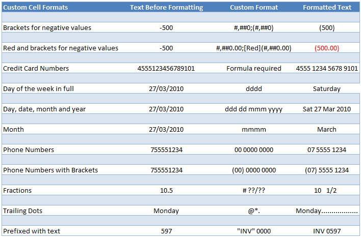
How to make your cell formats look the way you want
| Custom Cell Formats | Text Before Formatting | Custom Format | Formatted Text |
| Brackets for negative values | -500 | #,##0;(#,##0) | (500) |
| Red and brackets for negative values | -500 | #,##0.00;[Red](#,##0.00) | (500.00) |
| Day of the week in full | 27/03/2010 | dddd | Saturday |
| Day, date, month and year | 27/03/2010 | ddd dd mmm yyyy | Sat 27 Mar 2010 |
| Month | 27/03/2010 | mmmm | March |
| Phone Numbers | 755551234 | 00 0000 0000 | 07 5555 1234 |
| Phone Numbers with Brackets | 755551234 | (00) 0000 0000 | (07) 5555 1234 |
| Fractions | 10.5 | # ??/?? | 10 1/2 |
How to save time with Custom Cell Formats
1) From time to time I create a reference sheet like a contacts list, an index or even just a list of items like the one below using the custom cell format @*.

Because the text in the first column is often different lengths it can be hard for the eye to follow across. In these cases I like to use trailing dots to help the reader.
I wouldn’t dream of manually entering the dots but since I can create a custom format it’s worth it, plus I think it looks more elegant that using borders for this purpose as they can get a bit busy.
The custom cell format for trailing dots is @*. When you type in your text Excel will automatically enter the dots to fill to the end of the cell.
Tip: You’re not just limited to dots. You can have —- or **** or ____ or almost anything you want. Just replace the dot in the custom format with the character of your choice.
2) The other custom format I use regularly is prefixing my data with text. For example, I keep a record of our invoices and instead of typing ‘INV’ before each number I enter I use a custom cell format like this: “INV” 0000
Then when I type in 597 Excel converts it to INV 0597.
Tip: Replace INV with different text to suit your needs. It might be PO for purchase order, or any other text you can think of. Or make the text a suffix by changing the custom format to 0000 «INV».
Remember that even though the text appears to be INV 0597, for the purpose of formulas it’s still just a number 597.

Formatting cells for credit card numbers
You might be thinking you can use a custom format of 0000 0000 0000 0000 for credit card numbers, but you’ll find that it will only work for cards where the last number of the card is a zero! Try it out and see for yourself.
The workaround is to use a formula. This requires entering the number in one cell, and then in another cell you need to enter the following formula (assuming our credit card number is in cell A1):
=LEFT(A1,4) & " " & MID(A1,5,4) & " " & MID(A1,9,4) & " " & RIGHT(A1,4)
Note: I’ve added spaces in the formula for clarity.
Some explanation:
- The LEFT, MID and RIGHT returns text from a specified position in a cell.
- The ampersands ‘&’ join text together
- The “ “ adds a space between each group of text
[UPDATE] — You can also use this custom number format for credit cards and long phone numbers:
[<=99999999999]##########;#### #### #### ####
Thanks to MF for sharing that tip.
Enter your email address below to download the sample workbook.
By submitting your email address you agree that we can email you our Excel newsletter.
Excel includes a variety of built-in formats that cover general, numeric, currency, percentage, exponential, date, time, and custom numeric formats. You can also design custom formats based on one of the built-in formats.

To define a custom format, follow these steps:
1. Enter sample text for the format in a cell, and then select that cell (Excel then displays the sample text in the new format, which helps see the effects of your changes).
2. Do one of the following:
- Right-click on the selection and choose Format Cells… in the popup menu:

- On the Home tab, in the Number group, click the dialog box launcher:

- Press Ctrl+1.

3. In the Format Cells dialog box:
- On the Number tab, in the Category box, select the Custom item:

- In the Type list box, select the custom format you want to base your new custom format. Excel displays the details for the type in the Type text box.
- If the details for the type extend beyond the Type text box, double-click in the Type text box to select all its contents, issue a Copy command (for example, press Ctrl+C), and then paste the copied text into a text editor, such as Notepad. (For a shorter type, you can work effectively in the Type text box. For a longer type, it’s easier to have enough space to see the whole type at once.)
- Enter the details for the four parts of the type, separating the
parts from each other with a semicolon:- If you write formats with conditions such as [< 1000] and [≥ 1000], the format for the calculated condition is applied,
- Otherwise:
- If you write two formats, the first applies to positive and zero values and the second applies to negative values
- If you write three formats, the first applies to positive values, the second to negative values, and the third to zero
- If you write four formats, they apply to positive, negative, zero, and text values, respectively:
<positive>; <negative>; [zero]; [text]
- If you’re working in a text editor, copy what you typed and paste it
into the Type text box. Check the sample text to make sure it seems to be correct. - Click the OK button.

Codes for custom number formats
| Code | Description |
|---|---|
| General | Displays the number in general format. |
| # | Displays only significant digits and does not display insignificant zeros. |
| 0 (zero) | Displays insignificant zeros if a number has fewer digits than the zeros in the format. |
| ? | Displays a space for insignificant zeros on either side of the decimal point so that the decimal points align when formatted in a fixed-width font.
It can also be used for fractions with different numbers of digits. |
| . | Decimal point. |
| % | Percent symbol. |
| , | Thousand separator. |
| E-, E+, e-, e+ | Scientific notation. |
| $, —, +, /, (, ), :, space | Displays this character. |
| * | Repeats the next character to fill the full width of the column:
|
| _ (underscore) | Leaves a space equal to the width of the next character. |
| “text” | Displays text enclosed in double quotes. |
| @ | Text placeholder. |
| [color] | Displays characters in the specified color – black, blue, cyan, green, magenta, red, white , or yellow . |
| [condition value] | Custom criteria for each number format section. |

See also this tip in French:
Format de cellule personnalisé.
Please, disable AdBlock and reload the page to continue
Today, 30% of our visitors use Ad-Block to block ads.We understand your pain with ads, but without ads, we won’t be able to provide you with free content soon. If you need our content for work or study, please support our efforts and disable AdBlock for our site. As you will see, we have a lot of helpful information to share.
In this article, we will learn How to custom format cell in Excel.
What is the Format cell option ?
Custom format option lets you change the format of the number inside the cell. This is required because excel reads date and Time as General numbers. Format cell option allows you to change in any of the given formats.
- General
- Number
- Currency
- Accounting
- Date
- Time
- Percentage
- Fraction
- Scientific
- Text
- Special
- Custom
Under the custom option you can use the type of format required.
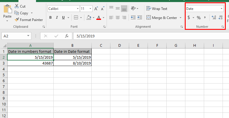
You can access the Format cell option in the Home tab to change the format as shown below.
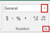
Just drop down from arrow and select from the view option or click the right most red box button as shown in the above image to open More number formats
There are some shortcuts to convert a number into different formats.
| Format | Shortcut key |
| General number | Ctrl + Shift + ~ |
| Currency format | Ctrl Shift $ |
| Percentage format | Ctrl Shift % |
| Scientific format | Ctrl + Shift + ^ |
| Date format | Ctrl + Shift + # |
| Time format | Ctrl + Shift + @ |
| Custom formats | Ctrl + 1 |
Example :
All of these might be confusing to understand. Let’s understand how to use the function using an example. Here we will see how one number can be seen many different formats.
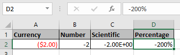
These are some of the format options of the number -2 in different formats.
Now there’s one more thing. Numbers represent so many values in a text as Date, Time and currency. So Sometimes you need to change the format cell type to required field type using Format cell option.

Use the format cell option shown below or Ctrl + 1 shortcut keyboard key that will open a full Format cell dialog box

Changing the format you will get
As you can see from the above snapshot that the number in general representation is converted to date format.
Here are all the observational notes using the custom format option in Excel
Notes :
- Use number formatting to convert the value into another format. The value remains the same.
- Use percentage format when using percentage rate values in Excel.
- Formula starts with ( = ) sign.
- Sometimes there exist a curly braces in the start of formula, which is an array formula and called using the Ctrl + Shift + Enter. Do not put curly braces manually.
- Text values and characters are always given using quotes or using cell reference
- Numerical values can be given directly or using the cell reference.
- Array can be given using the array reference or using named ranges.
Hope this article about How to custom format cell in Excel is explanatory. Find more articles on calculating values and related Excel formulas here. If you liked our blogs, share it with your friends on Facebook. And also you can follow us on Twitter and Facebook. We would love to hear from you, do let us know how we can improve, complement or innovate our work and make it better for you. Write to us at info@exceltip.com.
Related Articles :
How to use the Shortcut To Toggle Between Absolute and Relative References in Excel : F4 shortcut to convert absolute to relative reference and same shortcut use for vice versa in Excel.
How to use Shortcut Keys for Merge and Center in Excel : Use Alt and then follow h, m and c to Merge and centre cells in Excel.
How to Select Entire Column and Row Using Keyboard Shortcuts in Excel : Use Ctrl + Space to select whole column and Shift + Space to select whole row using keyboard shortcut in Excel
Paste Special Shortcut in Mac and Windows : In windows, the keyboard shortcut for paste special is Ctrl + Alt + V. Whereas in Mac, use Ctrl + COMMAND + V key combination to open the paste special dialog in Excel.
How to Insert Row Shortcut in Excel : Use Ctrl + Shift + = to open the Insert dialog box where you can insert row, column or cells in Excel.
50 Excel Shortcuts to Increase Your Productivity : Get faster at your tasks in Excel. These shortcuts will help you increase your work efficiency in Excel.
Excel REPLACE vs SUBSTITUTE function: The REPLACE and SUBSTITUTE functions are the most misunderstood functions. To find and replace a given text we use the SUBSTITUTE function. Where REPLACE is used to replace a number of characters in string…
Popular Articles :
How to use the IF Function in Excel : The IF statement in Excel checks the condition and returns a specific value if the condition is TRUE or returns another specific value if FALSE.
How to use the VLOOKUP Function in Excel : This is one of the most used and popular functions of excel that is used to lookup value from different ranges and sheets.
How to use the SUMIF Function in Excel : This is another dashboard essential function. This helps you sum up values on specific conditions.
How to use the COUNTIF Function in Excel : Count values with conditions using this amazing function. You don’t need to filter your data to count specific values. Countif function is essential to prepare your dashboard.