
Use AutoFilter or built-in comparison operators like «greater than» and “top 10” in Excel to show the data you want and hide the rest. Once you filter data in a range of cells or table, you can either reapply a filter to get up-to-date results, or clear a filter to redisplay all of the data.
Use filters to temporarily hide some of the data in a table, so you can focus on the data you want to see.

Filter a range of data
-
Select any cell within the range.
-
Select Data > Filter.

-
Select the column header arrow
. -
Select Text Filters or Number Filters, and then select a comparison, like Between.
-
Enter the filter criteria and select OK.

 .
.

Filter data in a table
When you put your data in a table, filter controls are automatically added to the table headers.

-
Select the column header arrow
for the column you want to filter. -
Uncheck (Select All) and select the boxes you want to show.
-
Click OK.
The column header arrow
changes to a Filter icon. Select this icon to change or clear the filter.
 for the column you want to filter.
 Filter icon. Select this icon to change or clear the filter.
Related Topics
Excel Training: Filter data in a table
Guidelines and examples for sorting and filtering data by color
Filter data in a PivotTable
Filter by using advanced criteria
Remove a filter
Filtered data displays only the rows that meet criteria that you specify and hides rows that you do not want displayed. After you filter data, you can copy, find, edit, format, chart, and print the subset of filtered data without rearranging or moving it.
You can also filter by more than one column. Filters are additive, which means that each additional filter is based on the current filter and further reduces the subset of data.
Note: When you use the Find dialog box to search filtered data, only the data that is displayed is searched; data that is not displayed is not searched. To search all the data, clear all filters.
The two types of filters
Using AutoFilter, you can create two types of filters: by a list value or by criteria. Each of these filter types is mutually exclusive for each range of cells or column table. For example, you can filter by a list of numbers, or a criteria, but not by both; you can filter by icon or by a custom filter, but not by both.
Reapplying a filter
To determine if a filter is applied, note the icon in the column heading:
-
A drop-down arrow
means that filtering is enabled but not applied.When you hover over the heading of a column with filtering enabled but not applied, a screen tip displays «(Showing All)».
-
A Filter button
means that a filter is applied.When you hover over the heading of a filtered column, a screen tip displays the filter applied to that column, such as «Equals a red cell color» or «Larger than 150».
When you reapply a filter, different results appear for the following reasons:
-
Data has been added, modified, or deleted to the range of cells or table column.
-
Values returned by a formula have changed and the worksheet has been recalculated.
Do not mix data types
For best results, do not mix data types, such as text and number, or number and date in the same column, because only one type of filter command is available for each column. If there is a mix of data types, the command that is displayed is the data type that occurs the most. For example, if the column contains three values stored as number and four as text, the Text Filters command is displayed .
Filter data in a table
When you put your data in a table, filtering controls are added to the table headers automatically.
-
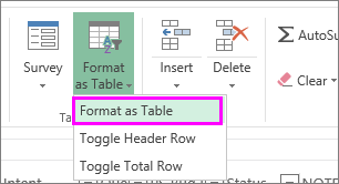
Select the data you want to filter. On the Home tab, click Format as Table, and then pick Format as Table.
-
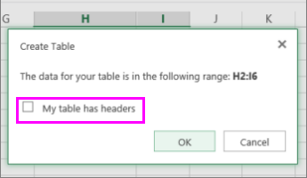
In the Create Table dialog box, you can choose whether your table has headers.
-
Select My table has headers to turn the top row of your data into table headers. The data in this row won’t be filtered.
-
Don’t select the check box if you want Excel for the web to add placeholder headers (that you can rename) above your table data.
-
-
Click OK.
-
To apply a filter, click the arrow in the column header, and pick a filter option.
Filter a range of data
If you don’t want to format your data as a table, you can also apply filters to a range of data.
-
Select the data you want to filter. For best results, the columns should have headings.
-
On the Data tab, choose Filter.
Filtering options for tables or ranges
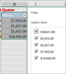
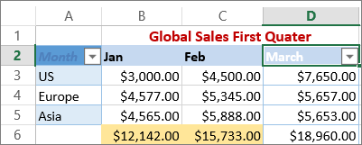
You can either apply a general Filter option or a custom filter specific to the data type. For example, when filtering numbers, you’ll see Number Filters, for dates you’ll see Date Filters, and for text you’ll see Text Filters. The general filter option lets you select the data you want to see from a list of existing data like this:
Number Filters lets you apply a custom filter:
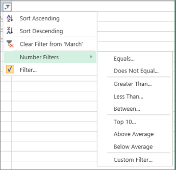
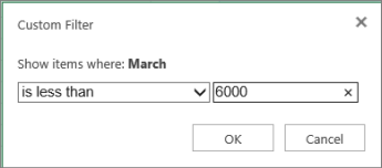
In this example, if you want to see the regions that had sales below $6,000 in March, you can apply a custom filter:
Here’s how:
-
Click the filter arrow next to March > Number Filters > Less Than and enter 6000.
-
Click OK.
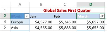
Excel for the web applies the filter and shows only the regions with sales below $6000.
You can apply custom Date Filters and Text Filters in a similar manner.
To clear a filter from a column
-
Click the Filter
button next to the column heading, and then click Clear Filter from <«Column Name»>.
To remove all the filters from a table or range
-
Select any cell inside your table or range and, on the Data tab, click the Filter button.
This will remove the filters from all the columns in your table or range and show all your data.
-
Click a cell in the range or table that you want to filter.
-
On the Data tab, click Filter.
-
Click the arrow
in the column that contains the content that you want to filter. -
Under Filter, click Choose One, and then enter your filter criteria.

 in the column that contains the content that you want to filter.
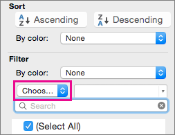
Notes:
-
You can apply filters to only one range of cells on a sheet at a time.
-
When you apply a filter to a column, the only filters available for other columns are the values visible in the currently filtered range.
-
Only the first 10,000 unique entries in a list appear in the filter window.
-
Click a cell in the range or table that you want to filter.
-
On the Data tab, click Filter.
-
Click the arrow
in the column that contains the content that you want to filter. -
Under Filter, click Choose One, and then enter your filter criteria.
-
In the box next to the pop-up menu, enter the number that you want to use.
-
Depending on your choice, you may be offered additional criteria to select:
Notes:
-
You can apply filters to only one range of cells on a sheet at a time.
-
When you apply a filter to a column, the only filters available for other columns are the values visible in the currently filtered range.
-
Only the first 10,000 unique entries in a list appear in the filter window.
-
Instead of filtering, you can use conditional formatting to make the top or bottom numbers stand out clearly in your data.
You can quickly filter data based on visual criteria, such as font color, cell color, or icon sets. And you can filter whether you have formatted cells, applied cell styles, or used conditional formatting.
-
In a range of cells or a table column, click a cell that contains the cell color, font color, or icon that you want to filter by.
-
On the Data tab, click Filter .
-
Click the arrow
in the column that contains the content that you want to filter. -
Under Filter, in the By color pop-up menu, select Cell Color, Font Color, or Cell Icon, and then click a color.
 in the column that contains the content that you want to filter.
This option is available only if the column that you want to filter contains a blank cell.
-
Click a cell in the range or table that you want to filter.
-
On the Data toolbar, click Filter.
-
Click the arrow
in the column that contains the content that you want to filter. -
In the (Select All) area, scroll down and select the (Blanks) check box.
Notes:
-
You can apply filters to only one range of cells on a sheet at a time.
-
When you apply a filter to a column, the only filters available for other columns are the values visible in the currently filtered range.
-
Only the first 10,000 unique entries in a list appear in the filter window.
-
-
Click a cell in the range or table that you want to filter.
-
On the Data tab, click Filter .
-
Click the arrow
in the column that contains the content that you want to filter. -
Under Filter, click Choose One, and then in the pop-up menu, do one of the following:
To filter the range for
Click
Rows that contain specific text
Contains or Equals.
Rows that do not contain specific text
Does Not Contain or Does Not Equal.
-
In the box next to the pop-up menu, enter the text that you want to use.
-
Depending on your choice, you may be offered additional criteria to select:
To
Click
Filter the table column or selection so that both criteria must be true
And.
Filter the table column or selection so that either or both criteria can be true
Or.
-
Click a cell in the range or table that you want to filter.
-
On the Data toolbar, click Filter .
-
Click the arrow
in the column that contains the content that you want to filter. -
Under Filter, click Choose One, and then in the pop-up menu, do one of the following:
To filter for
Click
The beginning of a line of text
Begins With.
The end of a line of text
Ends With.
Cells that contain text but do not begin with letters
Does Not Begin With.
Cells that contain text but do not end with letters
Does Not End With.
-
In the box next to the pop-up menu, enter the text that you want to use.
-
Depending on your choice, you may be offered additional criteria to select:
To
Click
Filter the table column or selection so that both criteria must be true
And.
Filter the table column or selection so that either or both criteria can be true
Or.
Wildcard characters can be used to help you build criteria.
-
Click a cell in the range or table that you want to filter.
-
On the Data toolbar, click Filter.
-
Click the arrow
in the column that contains the content that you want to filter. -
Under Filter, click Choose One, and select any option.
-
In the text box, type your criteria and include a wildcard character.
For example, if you wanted your filter to catch both the word «seat» and «seam», type sea?.
-
Do one of the following:
Use
To find
? (question mark)
Any single character
For example, sm?th finds «smith» and «smyth»
* (asterisk)
Any number of characters
For example, *east finds «Northeast» and «Southeast»
~ (tilde)
A question mark or an asterisk
For example, there~? finds «there?»
Do any of the following:
|
To |
Do this |
|---|---|
|
Remove specific filter criteria for a filter |
Click the arrow |
|
Remove all filters that are applied to a range or table |
Select the columns of the range or table that have filters applied, and then on the Data tab, click Filter. |
|
Remove filter arrows from or reapply filter arrows to a range or table |
Select the columns of the range or table that have filters applied, and then on the Data tab, click Filter. |
When you filter data, only the data that meets your criteria appears. The data that doesn’t meet that criteria is hidden. After you filter data, you can copy, find, edit, format, chart, and print the subset of filtered data.
Table with Top 4 Items filter applied
Filters are additive. This means that each additional filter is based on the current filter and further reduces the subset of data. You can make complex filters by filtering on more than one value, more than one format, or more than one criteria. For example, you can filter on all numbers greater than 5 that are also below average. But some filters (top and bottom ten, above and below average) are based on the original range of cells. For example, when you filter the top ten values, you’ll see the top ten values of the whole list, not the top ten values of the subset of the last filter.
In Excel, you can create three kinds of filters: by values, by a format, or by criteria. But each of these filter types is mutually exclusive. For example, you can filter by cell color or by a list of numbers, but not by both. You can filter by icon or by a custom filter, but not by both.
Filters hide extraneous data. In this manner, you can concentrate on just what you want to see. In contrast, when you sort data, the data is rearranged into some order. For more information about sorting, see Sort a list of data.
When you filter, consider the following guidelines:
-
Only the first 10,000 unique entries in a list appear in the filter window.
-
You can filter by more than one column. When you apply a filter to a column, the only filters available for other columns are the values visible in the currently filtered range.
-
You can apply filters to only one range of cells on a sheet at a time.
Note: When you use Find to search filtered data, only the data that is displayed is searched; data that is not displayed is not searched. To search all the data, clear all filters.
Need more help?
You can always ask an expert in the Excel Tech Community or get support in the Answers community.
Learning how to filter data in Excel enables you to find and work with just a subset of a larger list or database.
Filtering displays only the rows that contain a certain value or that meet a set criteria, while hiding other rows that don’t. Once you have filtered your data you can then work with just the visible set of data.
For example you might like to filter a list to find all sales made to one customer and then print only that data. Filter will allow you to do this in just a few clicks.
Applying the Excel Filter to your data
Before applying Filter to your data list make sure your list has field names (column headings).
1. Select the columns and rows that you want to filter, including the column headings.
Note: it is extremely important you make sure you have all of the data selected that you want included in the filter but avoid selecting the entire worksheet as this may slow down your filtering and you want to try to avoid getting the “whirly-wheel” on your screen. Only select the columns and rows that will be included in the filter.
2. On the Data tab in the Sort & Filter group click Filter.
3. Excel inserts a drop-down arrow next to each column label in your list. Click the arrow in the column that contains the data you want to filter.
4. A list of values will be displayed below the Search box. If a value is checked it will be displayed. Remove the check mark from any values you do not want displayed. Click OK.
The list will be filtered to only display records that meet your selection. A filter icon will be displayed on the drop-down arrow of the field(s) by which the list is filtered. If you place your mouse over the icon the filter setting will be displayed. Continue to add filters to as many columns as required.
Using the Search box to filter
Type keywords or phrases into the Search box to quickly locate list items. In the example below “top” has been typed into the Search box to find any list items containing the characters ‘top’. Use the Search box to quickly locate items when the list is long. It sure beats scrolling! It also makes sure you haven’t missed an item.
Remember that the Search box will always locate words that contain your search criteria. Wildcards can be used to locate items that begin or end with certain characters. For example a* would filter and display all items beginning with the letter “a” and * shop would find all items that end with the word “shop”.
Use the Add current selection to filter check box to search for multiple items and then append the selected item(s) to your current filter list.
Clearing filters
To remove a single filter click the arrow next to the column and select Clear Filter from the list, or on the Data tab, in the Sort & Filter group click the Clear button to remove all filters.
To remove Filter entirely from your data list, on the Data tab in the Sort & Filter group click Filter. Excel will remove the Filter drop-down arrows next to each column label in your list.
Filtering on columns containing numbers
- When it comes to filtering numbers, avoid checking and un-checking items in the filter list and instead click the Number Filters option on the Filter drop-down menu.
2. Select the option you require or click Custom Filter.
3. In the Custom AutoFilter dialog box, select the appropriate options and set the value(s) you want to use for each. In the example below the And option has been selected to filter the list to display any values that are greater than or equal to 500 AND less than or equal to 2000.
4. Once you have your criteria entered click OK and Excel will filter your list based on your custom settings.
Filtering on columns containing dates
- When it comes to filtering dates, you can easily check and un-check items in the filter list to include or exclude entire years, months or individual days. However if you would like to filter on a specific range of dates click the Date Filters option on the Filter drop-down menu.
2. Select the option you require or click Custom Filter. BTW, the date ranges for Quarter are from January to December and as far as I know these can’t be changes to suit.
3. In the Custom AutoFilter dialog box, select the appropriate options and set the date(s) you want to use for each. In the example below the the pop-up calendar at the end of each input box has been used to quickly insert the dates.
5. Once you have your criteria entered click OK and Excel will filter your list based on your custom settings.
When your total returns an error
If your total returns an error you may need to fix something within the data. Check our my post 5 Reasons why your Excel filter may not be working.
Working with the filtered data
When you filter data in Excel to display a subset of your data, your worksheet is in filter mode. In filter mode, many Excel commands operate only on the visible cells.
- Use the Copy and the Paste commands to place the copy of the filtered data wherever you want it, even in another workbook.
- Once you have filtered the data set select and then delete the rows to remove them from your data table.
- Select and apply formatting to the filtered data.
- Update the data quickly. For example, if we needed to change Pauls Top Shop to Paul’s Top Shop you can filter to only show Pauls Top Shop, update the row at the top of the list with the correct spelling and then copy it down the list. Remove filter once you are done.
Was this blog helpful? Let us know in the Comments below.
Advanced filter in Excel provides more opportunities for managing on data management spreadsheets. It is more complex in settings, but much more effective in action.
Using a standard filter, a Microsoft Excel user can solve not all of the tasks that are set. There is no visual display of the applied filtering conditions. It is not possible to apply more than two selection criteria. You can not filter the duplicate values to leave only unique records. And the criteria themselves are schematic and simple. The functionality of the extended filter is much richer. Let’s take a closer look at its possibilities.
How to make the advanced filter in Excel?
The advanced filter allows you to analysis data on an unlimited set of conditions. With this tool, the user can:
- to specify more than two selection criteria;
- to copy the result of filtering to another sheet;
- to set the condition of any complexity with the helping of formulas;
- to extract the unique values.
The algorithm for applying the extended filter is simple.
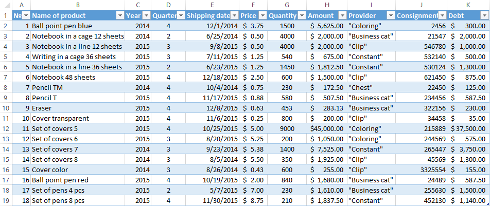
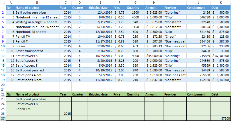
- To make the table with the original data or to open an existing one. Like so:
- To create the condition table. The features: the header line is the same with the «cap» of the filtered table. To avoid errors, need to copy the header line in the source table and paste it on the same sheet (side, top, underarm) or on another sheet. We enter the selection criteria into the condition table.
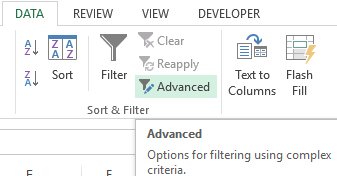
- Go to the «DATA» tab — «Sort and filter» — «Advanced». If the filtered information should be displayed on another sheet (NOT where the source table is), then you need to run the extended filter from another sheet.
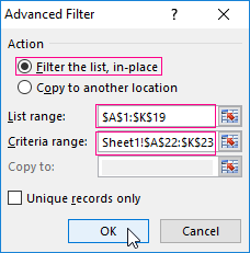
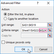
- In the «Advanced Filter» window that opens, to select the method of processing information (on the same sheet or on the other one), set the initial range (the table 1, example) and the range of conditions (the table 2, conditions). The header lines must be included in the ranges.
- To close the «Advanced Filter» window, click OK. We see the result.

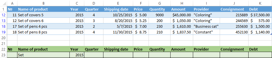
The top table is the result of the filtering. The lower nameplate with the conditions is given for clarity near.
How to use the advanced filter in Excel?
To cancel the action of the advanced filter, we place the cursor anywhere in the table and press Ctrl + Shift + L or «DATA» — «Sort and Filter» — «Clear».
We will find using the «Advanced Filter» tool information on the values that contain the word «Set».
In the table of conditions we bring in the criteria. For example, these are:

The program in this case will search for all information on the goods, in the title of which there is the word «Set».
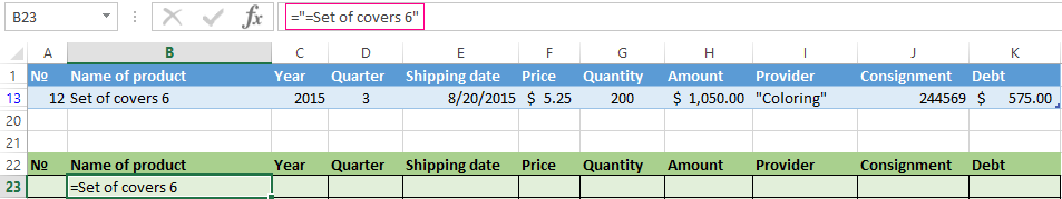
To search for the exact value, you can use the «=» sign. We enter the following criteria in the condition table:

Excel sees the «=» as a signal: the user will set the formula now. In order for the program to work correctly, the following should be written in the formula line: =»=Set of covers 6″.
After using the «Advanced Filter»:
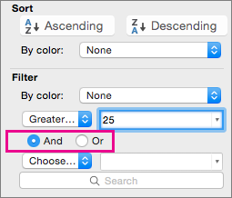
We filter the source table by the condition «OR» for different columns now. The operator «OR» is also in the tool «AutoFilter». But there it can be used within the single column.
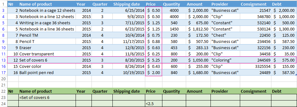
In the condition label we introduce the selection criteria: =»=Set of covers 6″. (In the column «Name of product») and = «<2.5$» (in the column «Price»). That is, the program must select those values that contain the EXACTLY information about the good «Set of covers 6 ». OR to the information about the goods, which price is <2.5.

Please note: the criteria must be written under the corresponding headings in the DIFFERENT lines.
The result of selection:
The advanced filter allows you to use as a criterion of a formula. Let’s consider the example.

Selection of the line with the maximum indebtedness: =MAX(Table1[Debt]).
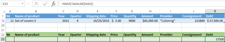
So we get the results as after running several filters on the one Excel sheet.
How to make few filters in Excel?
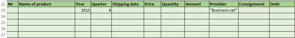
Let’s create the filter by several values. To do this, we enter in the table of conditions several criteria for selecting data:
Apply the tool «Advanced Filter»:
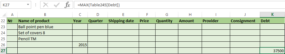
Now from the table with the selected data we will extract new information, which was selected according to other criteria. There are only shipping date for autumn 2015 (from September to November). Example:
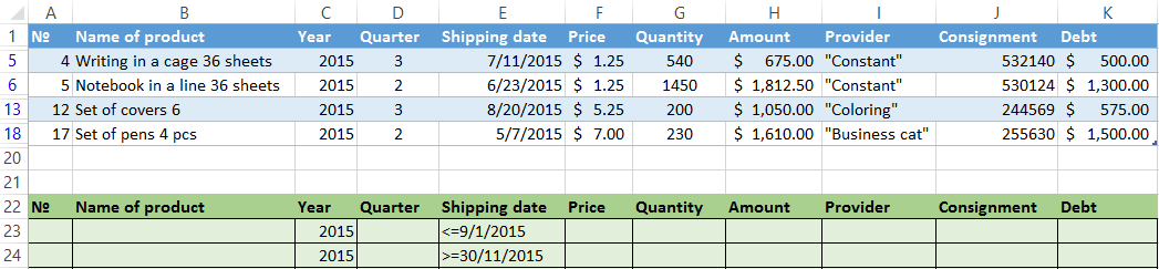
We introduce a new criterion in the condition table and apply the filtering tool. The initial range — is the table with data selected according to the previous criterion. This is how the filter is performed across on several columns.
To use few filters, you can create several condition tables on the new sheets. The method of implementation depends from the task which was set by user.
How to make the filter in Excel by lines?
By standard methods — you may not do it by any ways. Microsoft Excel selects data only in columns. Therefore, we need to look for other solutions.
Here are some examples of string criteria for the extended filter in Excel:
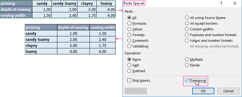
- Convert to the table. For example, from three rows make a list of three columns and apply the filtering to the transformed version.
- Use formulas to display exactly the data in the string that are needed. For example, make some indicator drop-down list. And in the next cell, enter the formula using the IF function. When a certain value is selected from the drop-down list, its parameter appears next to it.
To give an example of how the filter works by rows in Excel, we are creating the label:
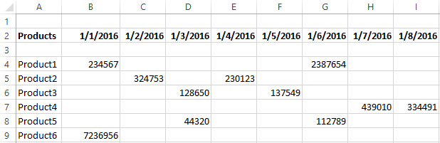
For the list of products, we create the drop-down list:
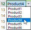
If necessary, learn how to create a drop-down list in Excel.
Above the table with the original data, we insert an empty line. In the cells, we introduce the formula that will show which columns the information is taken from.
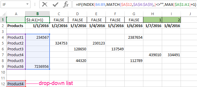
Next to the drop-down list box, we enter the following formula:
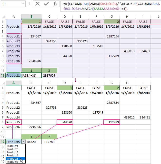
Its task is select from the table those values, that correspond to a certain good.
Download examples of advanced filtering
Thus, using the tool «Drop-down list» and built-in functions Excel selects data in rows according to a certain criterion.