Excel for Microsoft 365 Excel for Microsoft 365 for Mac Excel for the web More…Less
With the Currencies data type you can easily get and compare exchange rates from around the world. In this article, you’ll learn how to enter currency pairs, convert them into a data type, and extract more information for robust data.

Note: Currency pairs are only available to Microsoft 365 accounts (Worldwide Multi-Tenant clients.)
Use the Currencies data type to calculate exchange rates
-
Enter the currency pair in a cell using this format: From Currency / To Currency with the ISO currency codes.
For example, enter «USD/EUR» to get the exchange rate from one United States Dollar to Euros.
-
Select the cells and then select Insert > Table. Although creating a table isn’t required, it’ll make inserting data from the data type much easier later.
-
With the cells still selected, go to the Data tab and select the Currencies data type.
If Excel finds a match between the currency pair and our data provider, your text will convert to a data type and you’ll see the Currencies icon
in the cell.
Note: If you see
in the cell instead of the Currencies icon, then Excel is having difficulty matching the text with data. Correct any mistakes and press Enter to try again. Or, select the icon to open the Data Selector where you can search for a currency pair or specify the data you need.
-
To extract more information from the Currencies data type, select one or more converted cells and select the Insert Data button
that appears or press Ctrl/Cmd+Shift+F5.
-
You’ll see a list of all the fields available to choose from. Select the fields to add a new column of data.
For example, Price represents the exchange rate for the currency pair, Last Trade Time represents the time the exchange rate was quoted.
-
Once you have all the currency data that you want, you can use it in formulas or calculations. To ensure your data is up to date, you can go to Data > Refresh All to get an updated quote.
Caution: Currency information is provided «as-is» and may be delayed. Therefore, this data should not be used for trading purposes or advice. See About our data sources for more information.
See also
Stocks and geography data types
How to write formulas that reference data types
FIELDVALUE function
#FIELD! error
Need more help?
With Office 365, you can insert Exchange rate in your worksheets
The version of Excel in Office 365 allows you to collect the exchange rate of currencies of the current day.
Add Exchange Rate
The Office 365 version provides a great new feature ; Data Type. You just have to fill geographic data or financial data and Excel connects to a database to add values to the original one.
If you want to add financial data to the name of a stock holder or to return the exchange rate between 2 currencies, you just have to write your value in cells and then Click on the button Data > Stocks. You can use any separator ; space, dash, slash, pipe, …
What are the details behind the link
Once your have linked 2 currency to the Data Type tool, you can visualized all the informations in relationship between the 2 currencies by clicking on the icon
As you can see, behind a single connection between 2 currencies, you can return a lot of informations.
Return the last Exchange rate
What is amazing with Data Type, it’s the simplicity to return one of the data linked. To do that, you can click on the little rectangle in order to open the list of data you can add.
Or you can write a formula with a reference to the cell with the icon and then you press dot. Like that, you can also visualise all the information linked. Double-click or press Tab to select the option you want.
In both situation, the formula is
=D2.Price
Copy the dotted formula (beware of the format)
Like all the formulas in Excel, you can easily drag-and-drop the fill-handle to copy the formula.
But in this situation, you must take care of the currency format. Of course, when you copy the formula, you copy also the format of the original cell.
But you can force the each format by selecting the option Update Format.
Содержание
- Получить обменный курс валюты
- Использование типа данных «Валюты» для расчета обменных курсов
- Get a currency exchange rate
- Use the Currencies data type to calculate exchange rates
- Live and Historic Currency Exchange Rates in Excel
- Exchange rate in Excel
- With Office 365, you can insert Exchange rate in your worksheets
- Add Exchange Rate
- What are the details behind the link
- Return the last Exchange rate
- Copy the dotted formula (beware of the format)
- Currency exchange rate example
- Related functions
- Summary
- Generic formula
- Explanation
- Overview
- Basic currency exchange example
- Connecting the input cells
Получить обменный курс валюты
С помощью типа данных Валюты можно легко получить и сравнить обменные курсы по всему миру. В этой статье вы узнаете, как вводить пары валют, преобразовывать их в тип данных и извлекать дополнительные сведения для надежных данных.
Примечание: Валютные пары доступны только для Microsoft 365 (клиенты с несколькими клиентами по всему миру).
Использование типа данных «Валюты» для расчета обменных курсов
Введите валютную пару в ячейку, используя такой формат: Из валюты / В валюту с кодами валют ISO.
Например, введите «ДОЛЛАР/ЕВРО», чтобы получить курс обмена от одного доллара США к евро.
Выберем ячейки и выберите Вставить > таблицу. Создание таблицы не обязательно, но значительно упростит вставку данных из типа данных.
Выбрав ячейки, перейдите на вкладку Данные и выберите тип данных Валюты.
Если Excel обнаружит совпадение между валютной парой и поставщиком данных, текст преобразуется в тип данных, а в ячейке 
Примечание: Если в ячейке 
Чтобы извлечь дополнительные сведения из типа данных Валюты, выберите одну или несколько преобразованных ячеек и нажмите кнопку Вставить данные 
Вы увидите список всех доступных полей. Выберите поля, чтобы добавить новый столбец данных.
Например, «Цена» представляет обменный курс для валютной пары, а время последней сделки — время, в течение которого курс был цитироваться.
После того как у вас есть все необходимые данные о валюте, их можно использовать в формулахи вычислениях. Чтобы убедиться, что данные обновлены, перейдите в> Обновить все, чтобы получить обновленную кавычка.
Внимание: Сведения о валюте предоставляются «как есть» и могут быть задержаны. Поэтому эти данные не следует использовать в целях торговли или советов. Дополнительные сведения см. всведениях об источниках данных.
Источник
Get a currency exchange rate
With the Currencies data type you can easily get and compare exchange rates from around the world. In this article, you’ll learn how to enter currency pairs, convert them into a data type, and extract more information for robust data.
Note: Currency pairs are only available to Microsoft 365 accounts (Worldwide Multi-Tenant clients.)
Use the Currencies data type to calculate exchange rates
Enter the currency pair in a cell using this format: From Currency / To Currency with the ISO currency codes.
For example, enter «USD/EUR» to get the exchange rate from one United States Dollar to Euros.
Select the cells and then select Insert > Table. Although creating a table isn’t required, it’ll make inserting data from the data type much easier later.
With the cells still selected, go to the Data tab and select the Currencies data type.
If Excel finds a match between the currency pair and our data provider, your text will convert to a data type and you’ll see the Currencies icon 
Note: If you see 
To extract more information from the Currencies data type, select one or more converted cells and select the Insert Data button 
You’ll see a list of all the fields available to choose from. Select the fields to add a new column of data.
For example, Price represents the exchange rate for the currency pair, Last Trade Time represents the time the exchange rate was quoted.
Once you have all the currency data that you want, you can use it in formulas or calculations. To ensure your data is up to date, you can go to Data > Refresh All to get an updated quote.
Caution: Currency information is provided «as-is» and may be delayed. Therefore, this data should not be used for trading purposes or advice. See About our data sources for more information.
Источник
Live and Historic Currency Exchange Rates in Excel
Excel Price Feed is ideal for populating your Excel spreadsheet with live currency exchange rates.
Introduction
If you run an international business that deals in a variety of currencies or are simply trying to work out how much you spent on holiday then you have no doubt spent time updating a spreadsheet with the latest exchange rates.
This usually means looking up the rate on a website then copying/pasting the rate into a cell in your sheet. This process is repeated for each currency, and is repeated again whenever you want to update the fx rates (the fx market is open 24 hours a day).
There is an easier way, you can use the Excel Price Feed Add-in to automatically retrieve live exchange rates into Excel cells.
You set up the formula once and then each time you refresh your spreadsheet the latest live exchange rates are retrieved and the rate in the cell is updated.
Live Exchange Rates Example
After installing the Add-in you now have access to 100+ new Excel formulas, including the one below which will retrieve the live Euro / US Dollar (EUR/USD) exchange rate from Yahoo Finance:
This formula uses currency code of the exchange rate you require, the convention for Yahoo Finance is the currency pair code followed by «=X».
If you don’t know the currency code then you can use the search screen on the Configuration Pane, accessed from the button on the toolbar.
For this example we will start with a table of widgets that we are sourcing from 3 different countries which are priced in 3 different currencies:
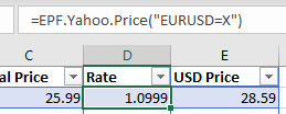
To populate the USD price column we just need to provide the live exchange rate to the «Rate» column, for example here we can see the EPF.Yahoo.Price formula used for the Euro widget in the Rate cell:
We repeat this formula for the next two rows, we now have the dollar price for each widget and can calculate a dollar total for all 3 widgets:
Any time you wish to update the exchange rates, simply press the «Refresh Sheet» button on the Excel Price Feed toolbar, no more copying/pasting exchange rates!
Historic Exchange Rates
Excel Price Feed also provides the ability to retrieve historic exchange rates into Excel cells. This is achieved using the EPF.Yahoo.Historic.Close formula.
For example, this formula will retrieve the Euro/US Dollar (EURUSD) exchange rate as it was on 1 January 2019:
Summary
We hope this tutorial really helps you save time building Excel spreadsheets that need live currency exchange rates.
Discover the power of Excel Price Feed with 80+ new Excel formulas for live, historic and fundamental data in your spreadsheet. Click the button below to request an Activation Code for your free 10 day trial:
Источник
Exchange rate in Excel
With Office 365, you can insert Exchange rate in your worksheets
The version of Excel in Office 365 allows you to collect the exchange rate of currencies of the current day.
Add Exchange Rate
The Office 365 version provides a great new feature ; Data Type. You just have to fill geographic data or financial data and Excel connects to a database to add values to the original one.
If you want to add financial data to the name of a stock holder or to return the exchange rate between 2 currencies, you just have to write your value in cells and then Click on the button Data > Stocks. You can use any separator ; space, dash, slash, pipe, .
What are the details behind the link
Once your have linked 2 currency to the Data Type tool, you can visualized all the informations in relationship between the 2 currencies by clicking on the icon

As you can see, behind a single connection between 2 currencies, you can return a lot of informations.
Return the last Exchange rate
What is amazing with Data Type, it’s the simplicity to return one of the data linked. To do that, you can click on the little rectangle in order to open the list of data you can add.
Or you can write a formula with a reference to the cell with the icon and then you press dot. Like that, you can also visualise all the information linked. Double-click or press Tab to select the option you want.
In both situation, the formula is
Copy the dotted formula (beware of the format)
Like all the formulas in Excel, you can easily drag-and-drop the fill-handle to copy the formula.
But in this situation, you must take care of the currency format. Of course, when you copy the formula, you copy also the format of the original cell.
But you can force the each format by selecting the option Update Format.
Источник
Currency exchange rate example
Summary
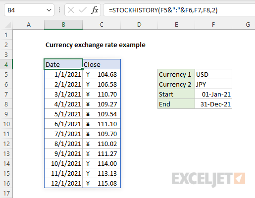
To get historical currency exchange rates over time, you can use the STOCKHISTORY function. In the example shown, the formula in cell B4 is:
The result is the monthly exchange rate for the USD > EUR currency pair shown in cells F5 and F6. Note that STOCKHISTORY returns an array of values that spill onto the worksheet into multiple cells. The STOCKHISTORY is only available in Excel 365.
Generic formula
Explanation
In this example, the goal is to get monthly currency exchange rates for a given currency pair (i.e. USD > EUR, USD > GBP, CAD > JPY, etc.). Currency abbreviations are entered in cells F5 and F6, and the start and end dates are entered in cells F7 and F8. If any of these four inputs are changed, the results seen in columns B and C will update dynamically. This can be done with the STOCKHISTORY function, whose purpose is to retrieve historical information for a financial instrument over time.
Overview
Although the name suggests otherwise, the STOCKHISTORY function can work with a variety of financial instruments, including bonds, index funds, mutual funds, bonds, and currency pairs. To work with currency exchange rates, STOCKHISTORY requires a currency pair entered as text.
STOCKHISTORY takes up to 11 arguments, most of which are optional. The syntax for the first 4 arguments looks like this:
Stock is a unique key for the instrument being retrieved, entered as a text value. For currency exchange rates, stock will be a currency pair like «USD:CAD». Start_date and end_date are Excel dates that define the time period being requested. Interval is the time interval – daily, weekly, or monthly. For a more complete description of all arguments and properties, see our STOCKHISTORY function page.
Basic currency exchange example
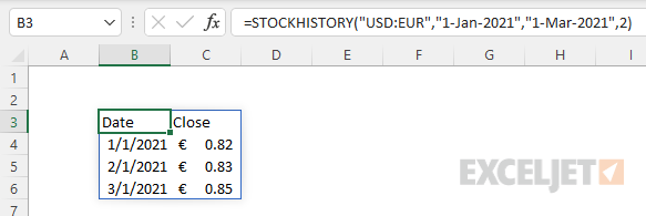
To get exchange rates for a given currency pair with STOCKHISTORY, enter the two 3-letter codes separated by a colon (:) as the stock argument. For example, to get the currency exchange rate between the US Dollar («USD») and the Euro («EUR») for the months of January 2021 through March 2021, you can use STOCKHISTORY like this:
In this example, the stock argument is the text value «USD:EUR», start_date is «1-Jan-2021», end_date is «1-Mar-2021». The interval argument specifies the time period to use between prices. The options are daily (0), weekly (1), or monthly (2). In this case, we want a monthly interval, so we provide 2. The result is an array with three months of rates:
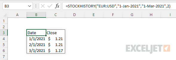
To reverse the direction of the exchange, just swap the order of the currency pairs:
Returns exchange rates in the opposite direction:
Note: in general, it’s safer to use the DATE function to enter dates in other formulas because it eliminates the risk of a text value being misinterpreted on other systems with different locale settings, but in this case dates are entered as text to keep things simple.
Connecting the input cells
To connect the basic formula above with the input cells in the example, shown, we need to substitute cell references for the hardcoded values. The final formula in cell B4 is:
Notice we assemble the stock argument by concatenating the currency symbols in cells F5 and F6 together, separated by a colon:
The result is fully dynamic. If any of these four inputs are changed, STOCKHISTORY will immediately return a new set of exchange rates. In the screen below, currency 1 has been set to «USD» (US Dollar) and currency 2 has been set to «JPY» (Japanese Yen):
The STOCKHISTORY function automatically sets the currency symbol as needed.
Note: when interval is set to monthly (2) as in this example, the STOCKHISTORY function will return the last available exchange rate in a given month.
Источник
In today’s business world, there is hardly any Excel workbook not using currencies and exchange rates. Example: When I want to know my revenue for the last month – let’s say of my Excel add-ins or books – I receive an Excel file containing data in various currencies. Because I’m located in Germany, I want to convert everything to Euro. That’s when the trouble starts: Which exchange rate do I use for example for converting US Dollar to Euro? And more importantly: Where do I get the currency exchange rate in a convenient and fast way?
Free sources
Let’s start with the possible sources. There are many sources for exchange rates online and the all offer them in a more or less convenient way. Here are some selected sources.
Google Finance
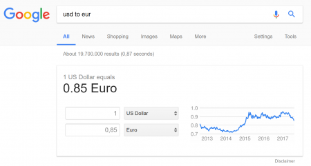
Actually there are two approaches with Google. The first one is just to use the standard Google search. Just type “USD to EUR” and you’ll receive the exchange rate.
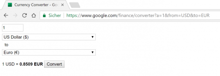
The second option has the advantage, that Google provides a very compact tool which you could use for some VBA automation. The link is quite straight-forward: https://www.google.com/finance/converter?a=1&from=USD&to=EUR. For converting other currencies than USD to EUR, just replace the respective symbols within the link. That’s it. You can furthermore define the amount by changing a=1 within the link: If you want to convert 2 USD to EUR, just say a=2 so that the complete link would be https://www.google.com/finance/converter?a=2&from=USD&to=EUR.
Yahoo!Finance
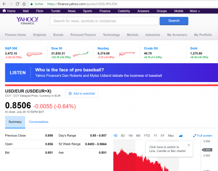
Similar to Google Finance, Yahoo!Finance also offers exchange rates. You can find them here:
https://finance.yahoo.com/quote/USDEUR%3DX
In this link, you can simply replace the USD and EUR symbols by other currencies. If you for example want to convert GBP to AUD, then the link would be
https://finance.yahoo.com/quote/GBPAUD%3DX
Oanda.com
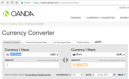
If you search for an exchange rate on a specific day, you could use oanda.com. The complete link is https://www.oanda.com/currency/converter/ and you can simple type your currencies and set the day (up to 180 days back).
Unfortunately, you can’t download time series of exchange rates for free. You’d need a Pro Account (75 USD per month). So if you just quickly need to look up an exchange rate within the last 180 days, this is a convenient tool. Otherwise you should rather use one of the other sources (below).
European Central Bank (ECB)
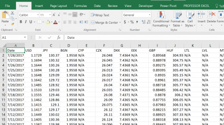
If you are looking for a free and comprehensive database, maybe one of the large banks is best for you. The European Central Bank offers daily exchange rates, always updated at 4 pm (CET). You can download the last 18 years as a CSV file.
- The link: https://www.ecb.europa.eu/stats/
policy_and_exchange_rates/
euro_reference_exchange_rates/html/index.en.html - The direct link for the CSV download: https://www.ecb.europa.eu/stats/
eurofxref/eurofxref-hist.zip
Please note the following comments:
- No current rates (please refer to Google or Yahoo! above).
- All rates are quoted against the Euro. So if you want to convert USD to GBP, you have to divide them yourself.
US Federal Reserve Bank
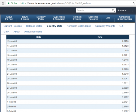
Similar to the ECB, the Federal Reserve Bank provides long time series of exchange rates. The format is not as handy as the CSV download of the ECB though.
The link: https://www.federalreserve.gov/releases/h10/hist/. You have to select your desired currency here first and get a long website for each currency.
How to work with exchange rates in Excel
Once you’ve found the exchange rates you need, there are some useful tips & tricks of how to integrate them into your Excel workbook. First you have to decide, if you want to use a fixed rate for all conversions or if you rather want to use daily rates.
Fixed rates
Fixed rates – that means you use the same rate for each currency conversion independent of the date – have one big advantage: They are much easier to integrate into your Excel sheet. Just find one rate (usually from either Google Finance, Yahoo!Finance or Oanda.com as shown above) and integrate it into your workbook.
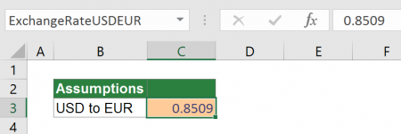
Please note the following advice: It’s recommended to set up one worksheet containing the basic assumptions. In this case, you’d have a worksheet containing all exchange rates. Whenever you use an exchange rate, link to the respective cell.
Also, try to name the cells, for example “ExchangeRateUSDEUR”. Now you can easily integrate the exchange rate into your formula: =A1*ExchangeRateUSDEUR
Daily rates
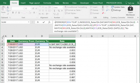
If you want to use daily exchange rates, you have to work a little bit harder. Recommendation: Download the exchange rates from the ECB. Open the CSV file by double-clicking on it and copy the sheet into your Excel workbook. Now use the 2-dimensional lookup INDEX/MATCH/MATCH for lookup up the exchange rate you need.
As you can see on the screenshot, the formula is quite long. Because all the exchange rates given in the CSV file are converting to EUR, you need to look up two exchange rates and divide them by each other.
Please feel free to download the example workbook here.
Do you want to boost your productivity in Excel?
Get the Professor Excel ribbon!
Add more than 120 great features to Excel!
Free Excel add-in for all currency exchange rates
– Update March 24, 2018 – Because Google removed the simple Google Finance website which provided the current exchange rates, we are switching to Yahoo Finance now. If your current version (1.0 and 1.1 of the add-in) have problems with the formula “PROFEXCurrentExchangeRate”, please download the current version below and use it instead.
We have a gift for you. Completely free! Our Excel add-in “Professor Excel Currency Converter”. Get up-to-date exchange rates directly into your Excel workbook. Once installed, you will see a new section on the right-hand side of the “Home” ribbon of Excel.

How to use the free Excel add-in
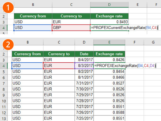
For installing the add-in, download the setup file below, click on it and follow the instructions.
Once installed, you can simply use it by typing these two formulas:
- =PROFEXCurrentExchangeRate(“USD”,”EUR”)
- =PROFEXExchangeRate(“USD”,
“EUR”,TODAY()-3)
Get the current exchange rate
The first formula, “=PROFEXCurrentExchangeRate(“USD”,”EUR”)” has two arguments: The currency from and the currency to. Quite simple, isn’t it?
Please note: The current exchange rates are only updated when you press the “Update Data” button. (The reason is, that – if you use it multiple times – your Excel might freeze if the exchange rates are updated permanently.)
Get historical exchange rates
The second formula =PROFEXExchangeRate(“USD”,”EUR”,TODAY()-3) has a three arguments:
- The currency from.
- The currency to.
- The date.
Very easy, isn’t it? You can further define within the settings, what happens if an exchange rate is not available (e.g. for weekends, public holidays):
- Either use the last available exchange rate.
- Or return an error message (“#VALUE!”)
Specifications in detail
- Sources: ECB rates for the historical rates and Google Finance Yahoo Finance exchange rates for the current rates.
- Updates: Rates are updated 4 pm each working day from ECB, live (some minutes delay though) from Google Finance Yahoo Finance.
- Period: Historical rates available from 4th of January 1999 until yesterday (not for all currencies though, check the ECB link above for more information).
- Currencies available:
| AUD | CNY | EEK | HUF | ISK | LVL | NOK | ROL | SGD | TRL |
| BGN | CYP | GBP | IDR | JPY | MTL | NZD | RON | SIT | TRY |
| BRL | CZK | HKD | ILS | KRW | MXN | PHP | RUB | SKK | USD |
| CAD | DKK | HRK | INR | LTL | MYR | PLN | SEK | THB | ZAR |
| CHF |
Download
Please feel free to download the Excel Curency Converter Add-In here: Download.
In this example, the goal is to get monthly currency exchange rates for a given currency pair (i.e. USD > EUR, USD > GBP, CAD > JPY, etc.). Currency abbreviations are entered in cells F5 and F6, and the start and end dates are entered in cells F7 and F8. If any of these four inputs are changed, the results seen in columns B and C will update dynamically. This can be done with the STOCKHISTORY function, whose purpose is to retrieve historical information for a financial instrument over time.
Overview
Although the name suggests otherwise, the STOCKHISTORY function can work with a variety of financial instruments, including bonds, index funds, mutual funds, bonds, and currency pairs. To work with currency exchange rates, STOCKHISTORY requires a currency pair entered as text.
STOCKHISTORY takes up to 11 arguments, most of which are optional. The syntax for the first 4 arguments looks like this:
=STOCKHISTORY(stock,start_date,[end_date],[interval])
Stock is a unique key for the instrument being retrieved, entered as a text value. For currency exchange rates, stock will be a currency pair like «USD:CAD». Start_date and end_date are Excel dates that define the time period being requested. Interval is the time interval – daily, weekly, or monthly. For a more complete description of all arguments and properties, see our STOCKHISTORY function page.
Basic currency exchange example
To get exchange rates for a given currency pair with STOCKHISTORY, enter the two 3-letter codes separated by a colon (:) as the stock argument. For example, to get the currency exchange rate between the US Dollar («USD») and the Euro («EUR») for the months of January 2021 through March 2021, you can use STOCKHISTORY like this:
=STOCKHISTORY("USD:EUR","1-Jan-2021","1-Mar-2021",2)
In this example, the stock argument is the text value «USD:EUR», start_date is «1-Jan-2021», end_date is «1-Mar-2021». The interval argument specifies the time period to use between prices. The options are daily (0), weekly (1), or monthly (2). In this case, we want a monthly interval, so we provide 2. The result is an array with three months of rates:
To reverse the direction of the exchange, just swap the order of the currency pairs:
=STOCKHISTORY("EUR:USD","1-Jan-2021","1-Mar-2021",2)
Returns exchange rates in the opposite direction:
Note: in general, it’s safer to use the DATE function to enter dates in other formulas because it eliminates the risk of a text value being misinterpreted on other systems with different locale settings, but in this case dates are entered as text to keep things simple.
Connecting the input cells
To connect the basic formula above with the input cells in the example, shown, we need to substitute cell references for the hardcoded values. The final formula in cell B4 is:
=STOCKHISTORY(F5&":"&F6,F7,F8,2)
Notice we assemble the stock argument by concatenating the currency symbols in cells F5 and F6 together, separated by a colon:
F5&":"&F6 // returns ""USD:EUR"
The result is fully dynamic. If any of these four inputs are changed, STOCKHISTORY will immediately return a new set of exchange rates. In the screen below, currency 1 has been set to «USD» (US Dollar) and currency 2 has been set to «JPY» (Japanese Yen):
The STOCKHISTORY function automatically sets the currency symbol as needed.
Note: when interval is set to monthly (2) as in this example, the STOCKHISTORY function will return the last available exchange rate in a given month.
If you use Microsoft Excel for financial data where exchange rates are part of what you need, check out the Currencies data type. This gives you various exchange details that you can include in your spreadsheet.
You can obtain the last trade time, high and low, change percent, and more by entering a pair of ISO currency codes. Then, simply select the details you want to include and refresh the data as needed.
Note: As of May 2022, the feature is only available to Microsoft 365 subscribers. You can use the feature in Excel for Microsoft 365 on Windows and Mac as well as Excel for the web.
Enter the Currency Pairs
You’ll enter a pair of currencies using the ISO codes as: From Currency / To Currency. You can use a colon instead of a slash if you prefer, but Excel will convert it to a slash when you apply the data type.
RELATED: How to Convert Currency in Microsoft Excel
So, to obtain the exchange rate and details from U.S. dollars to Euros, you would enter: USD/EUR. Or, for Australian dollars to U.S. dollars you would enter: AUD/USD.
Once you add the pair(s) you want to use, you’ll apply the data type and select the details to display.
Apply the Currencies Data Type
Select the cell where you entered the currency pair. Go to the Data tab and choose “Currencies” in the Data Types box.
You’ll see your cell update to display the data type icon on the left, indicating you’ve applied the Currencies type.
Note: If you see a question mark instead of the Currencies data type icon, that means Excel is having trouble matching the data you entered. Double-check the ISO codes for the currency types or click the question mark for more help.
Select the Exchange Data
With the currency pair cell selected, click the Insert Data icon that appears on the right. You’ll see a list of information that you can select from and insert into your sheet.
By default, the data you pick appears in the cell immediately to the right of the cell containing the currency pair. As you select more details to add, each one displays to the right as well.
Note this caution from Microsoft when obtaining currency exchange rates using this Excel feature:
Currency information is provided “as-is” and may be delayed. Therefore, this data should not be used for trading purposes or advice.
Refresh the Exchange Data
To have the most current details in your sheet, you can refresh the data as needed. For all items, go to the Data tab and click “Refresh All” in the Queries & Connections section of the ribbon.
For a particular item, select it and use the Refresh All drop-down arrow to pick “Refresh.”
If you like using the Currencies data type feature, take a look at how to use the Geography and Stocks options or even create your own data type!
READ NEXT
- › HoloLens Now Has Windows 11 and Incredible 3D Ink Features
- › BLUETTI Slashed Hundreds off Its Best Power Stations for Easter Sale
- › Google Chrome Is Getting Faster
- › The New NVIDIA GeForce RTX 4070 Is Like an RTX 3080 for $599
- › How to Adjust and Change Discord Fonts
- › This New Google TV Streaming Device Costs Just $20
How-To Geek is where you turn when you want experts to explain technology. Since we launched in 2006, our articles have been read billions of times. Want to know more?
Suppose you have some financial statistics in Microsoft Excel prepared in USD, and now the same is to be converted into Chinese Yuan.
How would you do it? This article is built to help you learn.
Excel doesn’t come packed with in-built currency conversion features.
However, you can easily convert your data to different currencies in Excel using either of the following methods discussed below.
More details into our Excel course offerings can be accessed here.
Why Convert your currency in Excel?
Excel is a powerful tool when it comes to calculations and processing of voluminous datasets. Given its versatility, you can use it nearly for any purpose.
Data that involves international currencies can get challenging in terms of currency conversion, especially if it is fine in magnitude. Although Excel doesn’t offer an in-built currency convertor, you can still use it to convert currency with ease.
Often businesses perform their bookkeeping exercises using Excel. They store data, including their sales and purchase records, in Excel. When the same data is to be made accessible to multiple regions, it may need to be converted into the functional currency of that region.
So will you prepare the records and summary financials from scratch only to present them in a different currency? With Excel, you don’t need to.
Simply build a currency conversion tool of your own through Power Query or use Kutools to present your data in any currency.
Learn more about currency conversion in Excel through the example below.
Converting currency using Formula – Simple Example
Converting currency in Excel requires a smart blend of external data sources (the up-to-date exchange rates) and a Pivot Table. Leave the rest to a basic multiplication formula.
Let’s see how you can convert currency in Excel using exchange rates found online through the example below.
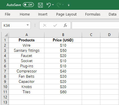
Following is a data set that constitutes different products and their prices in USD. The same needs to be converted into Euros. Here’s how you can do it.
Step 1:
To convert a currency using exchange rates found online, we need to import data into excel from an external web page. Do so by exporting data as follows:
Data > Get & Transform data > From Web
This opens up the dialogue box as follows.
Paste the URL of the address from where you want the data imported and click ‘Okay’ to have the data loaded to Excel.
Once you have loaded the data, you may want to filter out a specific exchange rate only. The same can be done using Advanced filters in Excel.
Step 2:
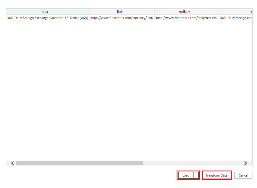
If the data is ready to be loaded into Excel with no adjustments required, click ‘Load data.’ Otherwise, choose ‘Transform Data’ as follows.
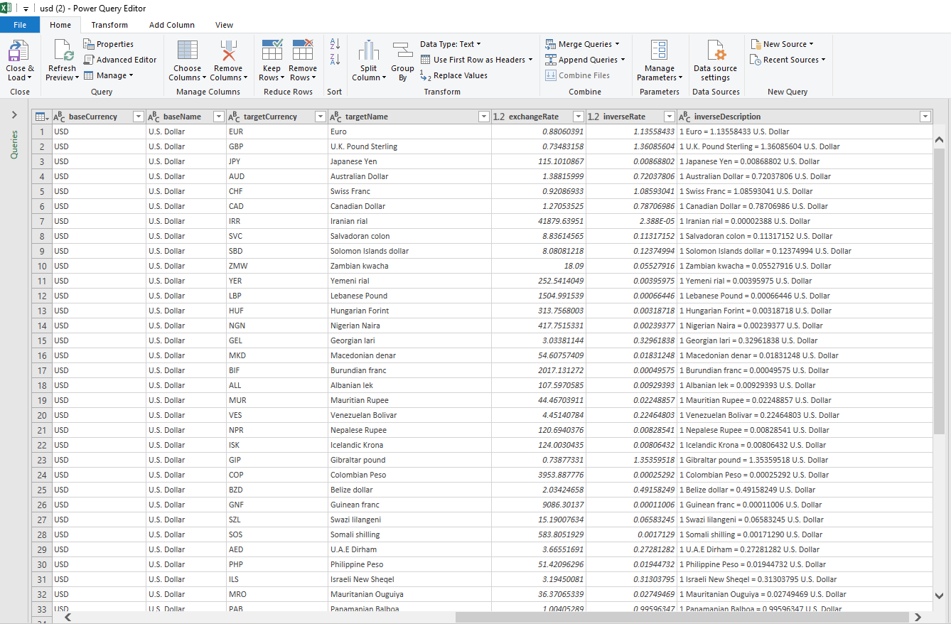
This launches the Power Query editor, where you can further edit the data to your choice. Learn more about Power Query here.
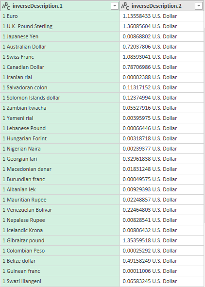
For instance, the data we’ve loaded consists of the rates as shown below.
However, we need the exchange rate in a separate column to apply the multiplication function. So, we can split the column in Power Query editor before loading it into Excel.
To do so, select the Exchange rate column and go as below.
Transform > Split Column > By Delimiter
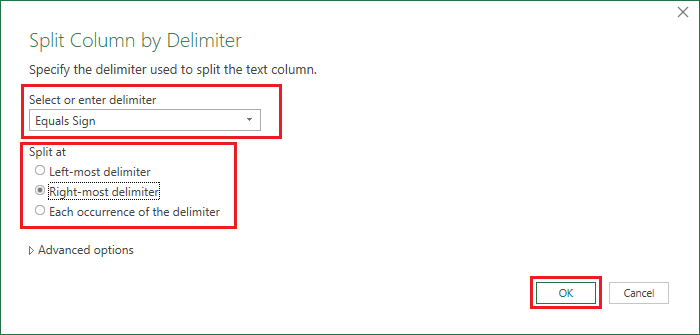
This takes you to the Split Column by Delimiter window, where you may select the delimiter.
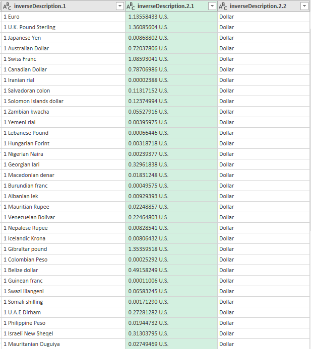
As shown above, we have selected ‘Equals Sign’ as the Delimiter and ‘Right Most Delimiter’ for delimiting. This is because we only want the exchange rate appearing on the rightmost to be separated.
This splits the columns into two, as shown below.
However, we only need the exchange rates and not the ‘U.S. Dollar’ written next to it. Once again, split the column using the Delimiter ‘Space’ and the ‘Right Most Delimiter’ on the recently split column.
This separates the exchange rate into a separate column, as shown below.
Once your data is ready to be imported to Excel, click ‘Close and Load’ as appears on the top left of the Power Query Editor window.
Step 3:
Here you have your exchange rates from an external source ready for conversion. Let’s go back to the original dataset having the Euro Prices listed down.
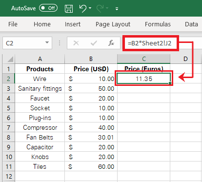
To have them converted in Euros, under the Euro column, feed the formula as follows.
=B2*Sheet2!J2
-
- B2 represents the USD value that needs to be converted into Euros
- Sheet2!J2 represents an absolute cell reference from the Exchange Rate sheet loaded into Excel.
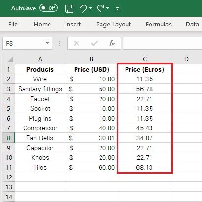
Drag and Drop to apply the same to all the products in the list.
Viola! There you have your currencies converted.
Step 4:
To make the currency differentiation more prominent, pair the figures with their respective currency symbol. For instance, to add the Euro symbol before to the currency listed under Column C, do as follows.
Select the figures > Number > Format Drop Down Menu > More Number formats
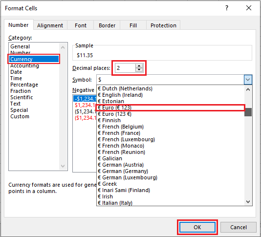
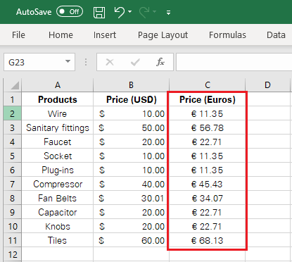
Select currency, select the Euro symbol from the dialogue box that opens up and restrict the decimal places to as many desired.
Symbols are added as follows.
Pro Tip: What if the exchange rates change in the future? Do we have to perform the entire exercise again? Obviously not.
Simply go to the sheet where the exchange rates are collated.
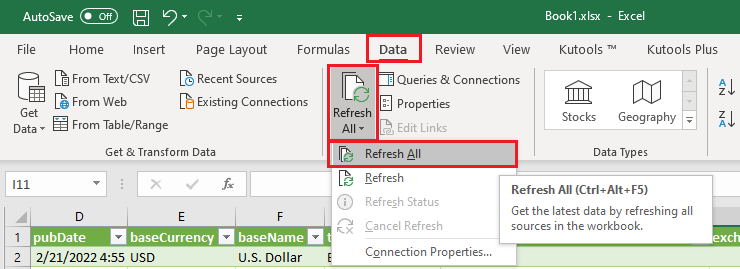
Go to Queries & Connections > Refresh All > Refresh All.
Excel would refresh the exchange rates imported from the web, and the formula applied to convert the currency would also be updated automatically. Want to know more about data modeling in Excel? Click here.
Kutools for Excel – Currency Tools
Kutools for Excel is not an in-built feature but an add-in that users would have to install for themselves. This handy add-in comes with over 300 advanced features to enhance your Excel experience multiple folds.
These features include a variety of one-click operations such as merging of cells without loss of data, data conversions, and much more. In addition, kutools save the mass time of Excel users by unburdening them of loads of complex work through smart functions.
Not only that, but it also enhances your work efficiency without you having to take specific Kutools training courses.
One of the most powerful features of Kutools is the currency conversion feature. It brings you an easy and efficient way of readily converting more than 50 currencies in Excel.
Kutools come embedded with the latest exchange rates from suitable online data sources. Be it a single value or volumes of data; you can have your data presented in various currencies only with a few clicks.
As Kutools source the latest exchange rates from the internet, it is essential to have a reliable internet connection at your end to employ this tool. This enables the ‘Update exchange rate’ option and makes the currency conversion feature work efficiently.
You may add the Kutool add-in to your Excel simply by downloading and installing it. No need to pay right away, as you can enjoy a free 30-day trial to see if the add-in works fine for you.
Converting currency using Kutools
Take it from us – converting currency gets way more manageable when done through Kutools. How? Kutools rids excel users of the tedious exercise to search for exchange rates.
As Kutools have the latest exchange rates fed in, you do not need to search for it from an online source or import it in Excel.
To learn how to convert currency in Excel using Kutools, follow the example below.
Continuing the same example as above, we have the price list of different products where the prices are listed in USD. Again, the same is to be converted into Euros.
Step 1:
Copy and paste the column containing the USD price to another adjacent column. Change the column header to the target currency post-conversion.
For instance, in the given example, we have copied and pasted the column’ Price (USD)’ and have changed the column name to ‘Price (Euros).’
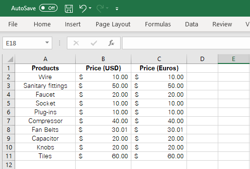
This is to be done as Kutools would convert USD into Euros in the original column, and therefore, the USD values will be replaced with Euro values. The original USD data will thus be lost.
If you want to simultaneously preserve both the USD and Euro columns in your worksheet, it is important to follow this step.
Step 2:
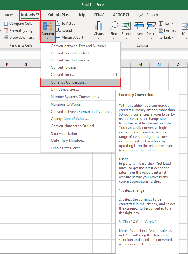
Select the column for the currency post-conversion i.e., Column C in our example, and launch the Kutools currency conversion tools.
Kutools > Content > Currency Conversion
Note: Kutool for Excel is an add-in that needs to be installed and enabled in Excel. If you don’t see the Kutools or Kutools Plus tab anywhere on the Ribbon, you probably don’t have it in your Excel.
Not to worry, you can easily download it and enable it to have the same added to Excel.
Step 3:
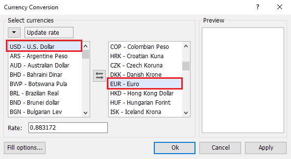
This opens up the following window.
The preceding window exhibits two currency boxes. The first one represents the currency of the original data (i.e., USD in our example).
The second currencies’ box represents the conversion currency (i.e., Euros in our example).
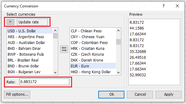
After selecting both the currencies from the respective boxes, click the update rate button as shown above.
This fetches the latest USD to Euro exchange rate.
Step 4:
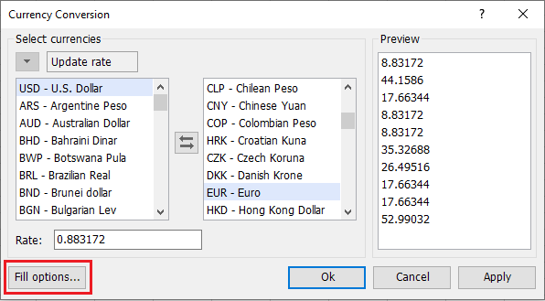
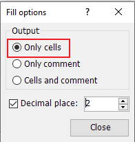
Next, click the ‘Fill Options’ button as it appears on the bottom left.
This opens up the following dialogues box, where you may select either of the three options.
-
-
Only Cells
-
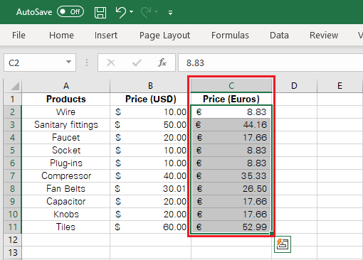
Choose the option ‘Only Cells’ and press close.
Click ‘okay’ from the currency conversion window as follows.
This option replaces the original prices with the converted currency. As evident from the screenshot above, Excel has replaced the USD Price values with Euro Price values.
-
-
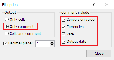
Only Comments
-
Choose the option ‘Only Comments,’ check the options on the right, and press close as follows.
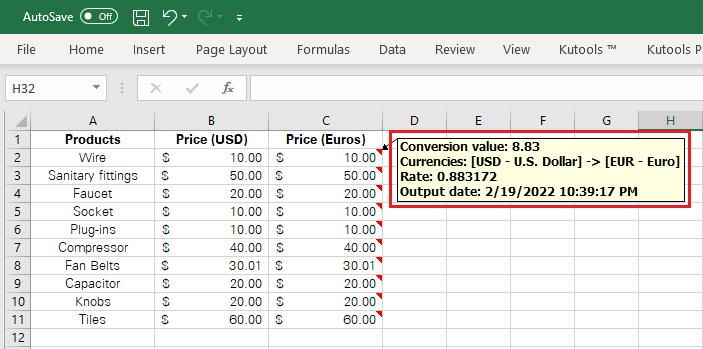
Click ‘okay’ from the currency conversion window to yield results.
This option doesn’t replace the original prices with the converted currency but only adds a comment that describes the conversion. For example, as evident from the screenshot above, Excel hasn’t replaced the USD Price values with Euro Price values, but only comment is added to each converted value.
-
-
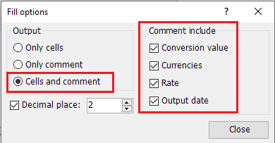
Cells and Comment
-
Choose the option ‘Cells and Comment’ and press close.
Click ‘okay’ from the currency conversion window as follows.
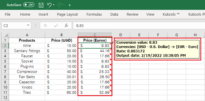
This option replaces the original prices with the converted currency and adds a comment that describes the conversion. As evident from the screenshot above, Excel has replaced the USD Price values with Euro Price values and has added a comment to each converted value.
There you are – converting currencies using Kutools is only that simple and quick. Kutools readily offer exchange rates for more than 50 currencies. These rates are imported from reliable internet sources.
Using Kutools, you can instantly convert a single value or multiple values to a different currency.
For more Excel tips, read our guide here on Recovering Unsaved Files.
Troubleshooting when converting currencies
The currency that makes the foundation of a dataset can cause it to be erroneous if not rightly converted. However, both the above-discussed methods would most likely not land you into problems when used for currency conversion in Excel.
However, the following currency conversion errors are often confronted by users. Here’s how you can deal with them.
1. Inappropriate format of the imported data
If you are going with option one, i.e., to import exchange rates from an online source for currency conversion, you need to pay special attention to quite a few things.
Often imported currency rates come in an inappropriate format i.e., anything other than numbers.
When the same is used for multiplication and currency conversion, Excel fails to apply the operation and returns a #VALUE! Error.
You can avoid this problem by ensuring that the exchange rates are formatted as numbers.
2. Unnecessary characters in the imported data
Other times, data imported into Excel comes together with a lot of fluff, be it empty spaces, unique characters, or parenthesis.
When you use the same to perform the currency conversion operation, Excel fails to do so and returns a #VALUE! Error or #REF! Error.
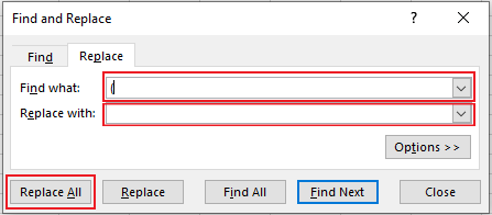
To cleanse the imported data of unwanted characters, you may use the ‘Find and Replace’ function. For example, if the imported data consists of unnecessary parenthesis, you may select the column where the data is populated and perform the ‘Find and Replace’ function as follows.
Excel would thus replace the parentheses with nothing i.e., these would be removed.
Conclusion
Though Excel doesn’t offer a currency-conversion tool, you can still convert currencies in Excel using different methods. Try applying these conversion techniques to your data to see how these methods make currency conversion in Excel a seamless experience.


