
Excel for Microsoft 365 Excel for Microsoft 365 for Mac Excel for the web Excel 2021 Excel 2021 for Mac Excel 2019 Excel 2019 for Mac Excel 2016 Excel 2016 for Mac Excel 2013 Excel 2010 Excel 2007 Excel for Mac 2011 More…Less
Array formulas are powerful formulas that enable you to perform complex calculations that often can’t be done with standard worksheet functions. They are also referred to as «Ctrl-Shift-Enter» or «CSE» formulas, because you need to press Ctrl+Shift+Enter to enter them. You can use array formulas to do the seemingly impossible, such as
-
Count the number of characters in a range of cells.
-
Sum numbers that meet certain conditions, such as the lowest values in a range or numbers that fall between an upper and lower boundary.
-
Sum every nth value in a range of values.
Excel provides two types of array formulas: Array formulas that perform several calculations to generate a single result and array formulas that calculate multiple results. Some worksheet functions return arrays of values, or require an array of values as an argument. For more information, see Guidelines and examples of array formulas.
Note: If you have a current version of Microsoft 365, then you can simply enter the formula in the top-left-cell of the output range, then press ENTER to confirm the formula as a dynamic array formula. Otherwise, the formula must be entered as a legacy array formula by first selecting the output range, entering the formula in the top-left-cell of the output range, and then pressing CTRL+SHIFT+ENTER to confirm it. Excel inserts curly brackets at the beginning and end of the formula for you. For more information on array formulas, see Guidelines and examples of array formulas.
This type of array formula can simplify a worksheet model by replacing several different formulas with a single array formula.
-
Click the cell in which you want to enter the array formula.
-
Enter the formula that you want to use.
Array formulas use standard formula syntax. They all begin with an equal sign (=), and you can use any of the built-in Excel functions in your array formulas.
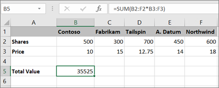
For example, this formula calculates the total value of an array of stock prices and shares, and places the result in the cell next to «Total Value.»

The formula first multiplies the shares (cells B2 – F2) by their prices (cells B3 – F3), and then adds those results to create a grand total of 35,525. This is an example of a single-cell array formula because the formula lives in just one cell.
-
Press Enter (if you have a current Microsoft 365 Subscription); otherwise press Ctrl+Shift+Enter.
When you press Ctrl+Shift+Enter, Excel automatically inserts the formula between { } (a pair of opening and closing braces).
Note: If you have a current version of Microsoft 365, then you can simply enter the formula in the top-left-cell of the output range, then press ENTER to confirm the formula as a dynamic array formula. Otherwise, the formula must be entered as a legacy array formula by first selecting the output range, entering the formula in the top-left-cell of the output range, and then pressing CTRL+SHIFT+ENTER to confirm it. Excel inserts curly brackets at the beginning and end of the formula for you. For more information on array formulas, see Guidelines and examples of array formulas.
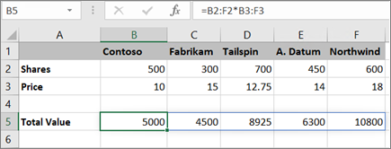
To calculate multiple results by using an array formula, enter the array into a range of cells that has the exact same number of rows and columns that you’ll use in the array arguments.
-
Select the range of cells in which you want to enter the array formula.
-
Enter the formula that you want to use.
Array formulas use standard formula syntax. They all begin with an equal sign (=), and you can use any of the built-in Excel functions in your array formulas.
In the following example, the formula multiples shares by price in each column, and the formula lives in the selected cells in row 5.
-
Press Enter (if you have a current Microsoft 365 Subscription); otherwise press Ctrl+Shift+Enter.
When you press Ctrl+Shift+Enter, Excel automatically inserts the formula between { } (a pair of opening and closing braces).
Note: If you have a current version of Microsoft 365, then you can simply enter the formula in the top-left-cell of the output range, then press ENTER to confirm the formula as a dynamic array formula. Otherwise, the formula must be entered as a legacy array formula by first selecting the output range, entering the formula in the top-left-cell of the output range, and then pressing CTRL+SHIFT+ENTER to confirm it. Excel inserts curly brackets at the beginning and end of the formula for you. For more information on array formulas, see Guidelines and examples of array formulas.
If you need to include new data in your array formula, see Expand an array formula. You can also try:
-
Rules for changing array formulas (they can be finicky)
-
Delete an array formula (you press Ctrl+Shift+Enter there, too)
-
Use array constants in array formulas (they can be handy)
-
Name an array constant (they can make constants easier to use)
If you want to play around with array constants before you try them out with your own data, you can use the sample data here.
The workbook below shows examples of array formulas. To best work with the examples, you should download the workbook to your computer by clicking the Excel icon in the lower-right corner, and then open it in the Excel desktop program.
Copy the table below and paste it into Excel in cell A1. Be sure to select cells E2:E11, enter the formula =C2:C11*D2:D11, and then press Ctrl+Shift+Enter to make it an array formula.
|
Salesperson |
Car Type |
Number Sold |
Unit Price |
Total Sales |
|---|---|---|---|---|
|
Barnhill |
Sedan |
5 |
2200 |
=C2:C11*D2:D11 |
|
Coupe |
4 |
1800 |
||
|
Ingle |
Sedan |
6 |
2300 |
|
|
Coupe |
8 |
1700 |
||
|
Jordan |
Sedan |
3 |
2000 |
|
|
Coupe |
1 |
1600 |
||
|
Pica |
Sedan |
9 |
2150 |
|
|
Coupe |
5 |
1950 |
||
|
Sanchez |
Sedan |
6 |
2250 |
|
|
Coupe |
8 |
2000 |
Create a multi-cell array formula
-
In the sample workbook, select cells E2 through E11. These cells will contain your results.
You always select the cell or cells that will contain your results before you enter the formula.
And by always, we mean 100-percent of the time.
-
Enter this formula. To enter it in a cell, just start typing (press the equal sign) and the formula appears in the last cell you selected. You can also enter the formula in the formula bar:
=C2:C11*D2:D11
-
Press Ctrl+Shift+Enter.
Create a single-cell array formula
-
In the sample workbook, click cell B13.
-
Enter this formula using either method from step 2 above:
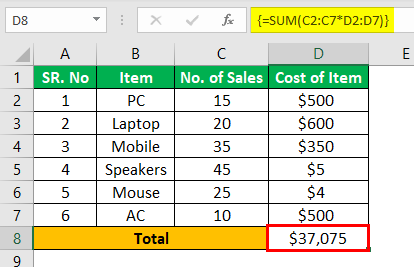
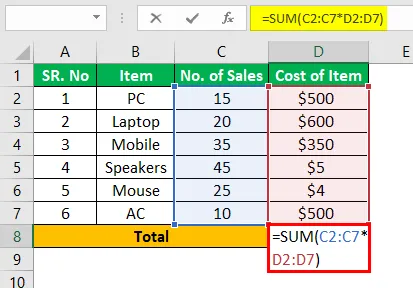
=SUM(C2:C11*D2:D11)
-
Press Ctrl+Shift+Enter.
The formula multiplies the values in the cell ranges C2:C11 and D2:D11, then adds the results to calculate a grand total.
In Excel for the web, you can view array formulas if the workbook you open already has them. But you won’t be able to create an array formula in this version of Excel by pressing Ctrl+Shift+Enter, which inserts the formula between a pair of opening and closing braces({ }). Manually entering these braces won’t turn the formula into an array formula either.
If you have the Excel desktop application, you can use the Open in Excel button to open the workbook and create an array formula.
Need more help?
You can always ask an expert in the Excel Tech Community or get support in the Answers community.
Need more help?
Ctrl Shift-Enter helps convert the data into an array format consisting of multiple data values in Excel. It also supports differentiation between the regular formula and array formula in excelArray formulas are extremely helpful and powerful formulas that are used in Excel to execute some of the most complex calculations. There are two types of array formulas: one that returns a single result and the other that returns multiple results.read more. Using this shortcut provides two major advantages: dealing with a set of values and returning the multiple values simultaneously.
For example, we can calculate the sales and costs of various electronic gadgets over any given number of years.
Ctrl+Shift+Enter is one of the shortcuts used in Excel to perform the calculations with array formulas. It supports performing complex calculations using the standard excel functionsExcel functions help the users to save time and maintain extensive worksheets. There are 100+ excel functions categorized as financial, logical, text, date and time, Lookup & Reference, Math, Statistical and Information functions.read more. It is widely used in the array formulae to apply functions and formulas to a data set.
Table of contents
- Excel Ctrl Shift-Enter Command
- Explanation
- Examples of Ctrl Shift-Enter In Excel
- Example #1 – To Determine the Sum
- Example #2 – To Determine Sum using Condition
- Example #3 – To Determine the Inverse Matrix
- Applications
- Things to Remember
- Recommended Articles
Explanation
- Before we want to use the shortcut CTRL+SHIFT+ENTER, we need to understand more about the arrays. The array is the collection of the data, including text and numerical values in multiple rows and columns or only in a single row and column. For example, Array = {15, 25, -10, 24}
- To enter the above values into an array, we need to enter CTRL+SHIFT+ENTER after selecting the range of cells. It results in the array as:
- Array= {= {15, 25, -10, 24}}
- As shown above, braces are enclosed to the formula by resulting in the range of cells in a single horizontal array. This keyboard shortcutAn Excel shortcut is a technique of performing a manual task in a quicker way.read more works in different versions of Excel, including 2007, 2010, 2013, and 2016.
- CTRL+SHIFT+ENTER also works for vertical and multi-dimensional arrays in Excel. This shortcut works for different functions that require the use of data in a range of cells. It is effectively used in various operations like determining sums and performing matrix multiplication in excelThe MMULT function in Excel is an inbuilt function for matrix multiplication. It accepts two arrays as arguments and returns the product of the two arrays. read more.
Examples of Ctrl Shift-Enter In Excel
You can download this Ctrl Shift Enter Excel Template here – Ctrl Shift Enter Excel Template
Example #1 – To Determine the Sum
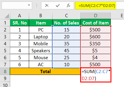
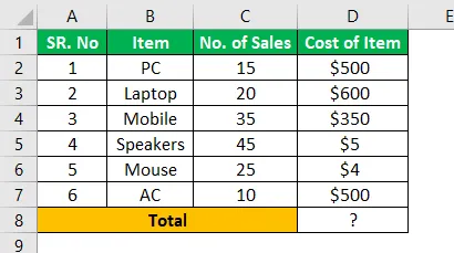
This example best illustrates the use of Ctrl+SHIFT+ENTER in calculating the sum of sales generated for different products. Therefore, the following data is considered for this example.

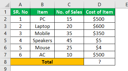
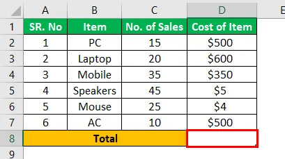
Step 1: First, we must place the cursor into the empty cell where we want to produce the worth of the product’s total sales.

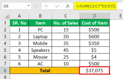
Step 2: As shown in the figure, we need to insert the formula as total = sum (D6:D11*E6: E11).

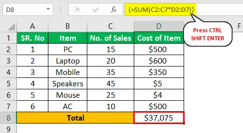
Step 3: After entering the formula, we must press CTRL+SHIFT +ENTER to convert the general formula into an array formula.
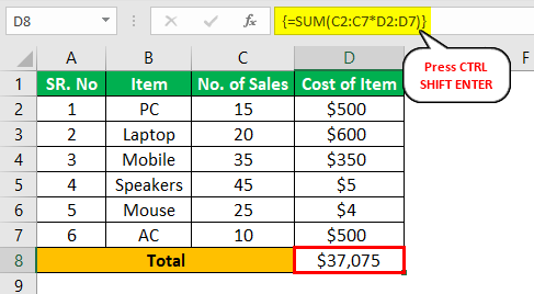
Step 4: As a result, the opening and closing braces are added to the sum formula in excelThe SUM function in excel adds the numerical values in a range of cells. Being categorized under the Math and Trigonometry function, it is entered by typing “=SUM” followed by the values to be summed. The values supplied to the function can be numbers, cell references or ranges.read more. The result will be obtained, as shown in the figure.
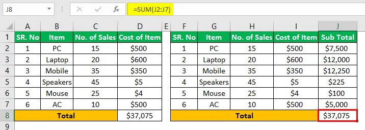
Step 5: Now, we need to check the result determining the total with the general procedure we used.

The result obtained from the two procedures is the same. But, using the array formula with CTRL+SHIFT+ENTER is easy to determine total sales by eliminating the calculation of an additional subtotal column.
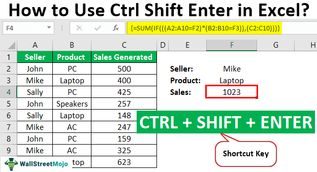
Example #2 – To Determine Sum using Condition
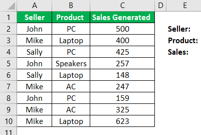
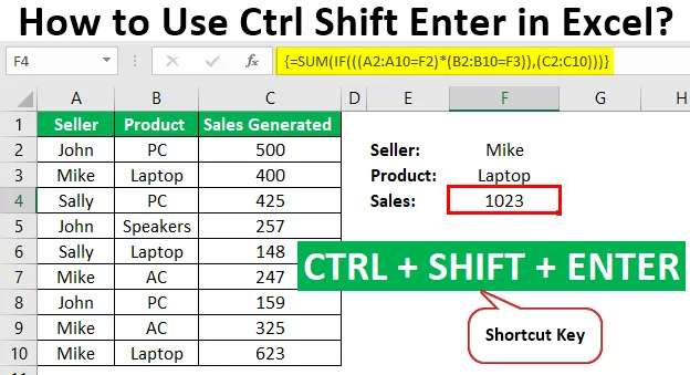
This example best illustrates the use of Ctrl+SHIFT+ENTER in calculating the sum of sales generated for different products using the conditions. Therefore, the following data is considered for this example.

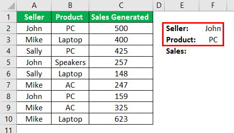
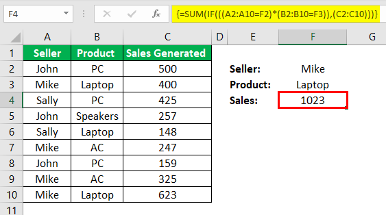
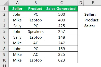
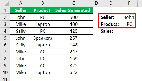
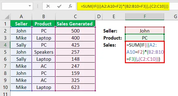
Step 1: In the first step, we need to determine the details of the seller and product that want to calculate sales generated individually. Consider Seller =John and Product = PC and enter these details into individual cells, as shown in the figure.
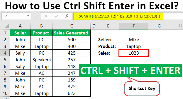
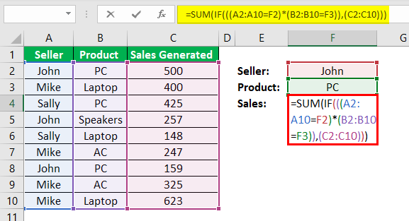
Step 2: To determine the sales generated by John in selling PC products, the formula as:
=SUM (IF (((A2:A10=F2)*(B2:B10=F3)), (C2:C10)))

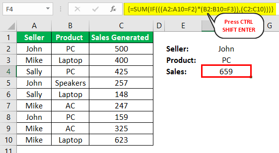
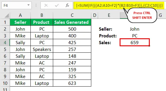
Step 3: We mustpress CTRL+SHIFT+ENTER to have the desired result, as shown in the figure.

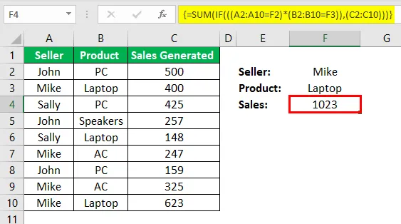
Step 4: Now, we need to change the values of F2 and F3 cells to determine sales generated by other persons.

In this way, the calculation of sales generated is automated using the shortcut CTRL+SHIFT+ENTER.
Example #3 – To Determine the Inverse Matrix
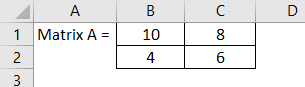
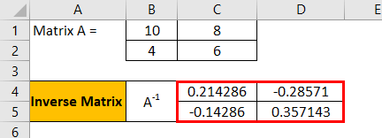
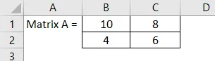
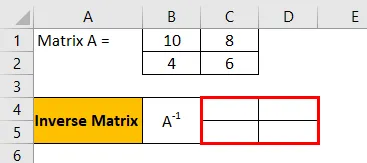
For this example, consider the following matrix A.
Let A = 10 8
4 6
Follow the below steps to get the inverse matrix.
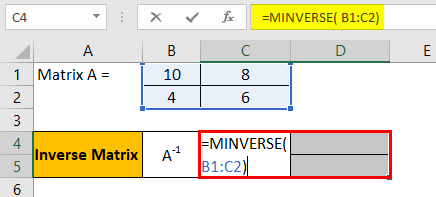
- Initially, we must enter the matrix A into the Excel sheet, as shown in the figure below.

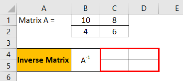
The range of the matrix is B1:C2. - Then, highlight the range of cells to position the inverse matrix in Excel A-1 on the same sheet.

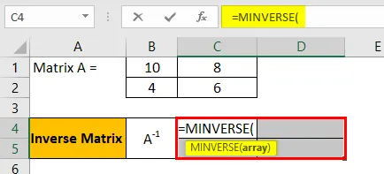
- After highlighting the range of cells, we must input the formula of MINVERSE to calculate the inverse matrix.
Ensure during inputting the formula that all cells are highlighted.

- First, we must enter the array or matrix range, as shown in the screenshot.

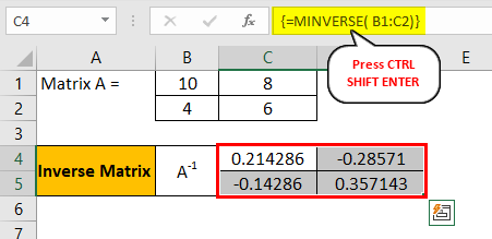
- Once the MINVERSE function is entered successfully, we must use the shortcut CTRL+SHIFT+ENTER to generate the array formula to have the results of all four matrix components without re-entering to other details.
The converted array formula is shown as
{=MINVERSE (B1: C2)}
- The resultant inverse matrix is produced as:

Applications
CTRL + SHIFT + ENTER is used in many applications in Excel.
- Creating an array formula in matrix operations such as multiplication.
- Creating an array formula in determining the sum of the set of values.
- Replacing the hundreds of formulas with only a single array formula or summing the range of data that meets specific criteria or conditions.
- To count the number of characters or values in the range of data in Excel.
- To sum the values presented in every nth column or row within low and upper boundaries.
- To perform the task of creating simple datasets in a short time.
- To expand the array formula to multiple cells.
- To determine the Average, Min, Max, Aggregate, and array expressions values.
- To return the results in multiple and single cells by applying the array formulas.
- To use CTRL+SHIFT+ENTER in the IF function in excelIF function in Excel evaluates whether a given condition is met and returns a value depending on whether the result is “true” or “false”. It is a conditional function of Excel, which returns the result based on the fulfillment or non-fulfillment of the given criteria.
read more.
Things to Remember
- The manual entering of braces surrounding the formula does not work in Excel. Instead, we should press the shortcut CTRL+SHIFT+ENTER.
- When we edit the array formula, we must press the shortcut CTRL+SHIFT+ENTER again since the braces are removed every time we change.
- Using the shortcut requires selecting the range of cells to result in the output before entering the array formula.
Recommended Articles
This article has been a guide to the Ctrl Shift-Enter in Excel. Here, we learn when and how to use Ctrl Shift-Enter in Excel, examples, and a downloadable template. You may learn more about Excel from the following articles: –
- How Many Rows and Columns in Excel?
- Break-Even Point in Excel
- Using String Array in VBA
- Declare Array in VBA
Ctrl Shift-Enter in Excel (Table of Contents)
- Explanation of Ctrl Shift-Enter in Excel
- Examples of Excel Control Shift-Enter
Excel Ctrl Shift-Enter
Ctrl Shift-Enter is one of the shortcuts used in Excel to perform the calculations with array formulae. It supports in performing complex calculation using the standard excel functions. It is widely used in the array formulae to apply functions and formulas on a set of data. The use of Ctrl Shift-Enter together helps in converting the data into an array format which consists of multiple data values in excel. It also supports in differentiation between the regular formula and array formula. With this shortcut, there are two major advantages, such as dealing with a set of values and returning the multiple values at a time.
Explanation of Ctrl Shift-Enter in Excel
- Before we use the shortcut CTRL SHIFT-ENTER, we need to understand more about the arrays. Arrays are the collection of the data, including text and numerical values in multiple rows and columns or only in a single row and column. For example, Array = {15, 25, -10, 24}.
- To enter the above values into an array, we need to enter CTRL SHIFT+ENTER after the selection of the range of cells. It results in the array as Array= {= {15, 25, -10, 24}}.
- As shown above, braces are enclosed to the formula by resulting in the range of cells in a single horizontal array. This keyboard shortcut works in different versions of Excel, including 2007, 2010, 2013, and 2016.
- CTRL SHIFT-ENTER also works for vertical and multi-dimensional arrays in Excel. This shortcut works for different functions that require the use of data in a range of cells. It is effectively used in various operations like determining sum and performing matrix multiplication.
How to Use Ctrl Shift-Enter in Excel?
CTRL SHIFT-ENTER is used in many applications in Excel.
You can download this CTRL Shift-Enter Excel Template here – CTRL Shift-Enter Excel Template
- Creation of array formula in matrix operations such as multiplication.
- Creation of array formula in determining the sum of the set of values.
- Replacing the hundreds of formulas with only a single array formula or summing the range of data that meets specific criteria or conditions.
- Counting the number of characters or values in the range of data in Excel.
- Summing the values presented in every nth column or row within low and upper boundaries.
- Performing the task of the creation of simple datasets in a short time.
- Expanding the array formula to multiple cells.
- Determining the Average, Min, Max, Aggregate, and array expressions.
- Returning the results in multiple and single cells applying the array formulas.
- Use of CTRL SHIFT-ENTER in IF functions.
Examples of Ctrl Shift-Enter in Excel
Below are the examples of excel control shift-enter.
Example #1 – To Determine Sum
This example illustrates the use of Ctrl SHIFT-ENTER in calculating the sum of sales generated for different products. The following data is considered for this example.
Step 1: Place the cursor in the empty cell where you want to produce the worth of the product’s total sales.

Step 2: Enter the formula as total = sum (D6:D11*E6: E11) as shown in the below image.
Step 3: After entering the formula, press CTRL SHIFT-ENTER to convert the general formula into an array formula.

Step 4: The opening and closing braces are added to the sum formula. The result is obtained as shown in the image.

Step 5: Check the result determining total with the general procedure we used.

The result obtained from the two procedures is the same. But, using the array formula with CTRL SHIFT ENTER is easy in determining total sales by eliminating the calculation of an additional column of the subtotal.
Example #2 – Determine the Sum using Condition
This example illustrates the use of Ctrl SHIFT-ENTER in calculating the sum of sales generated for different products using the conditions. The following data is considered for this example.
Step 1: In the first step, determine the details of the seller and product that want to calculate sales generated individually. Consider Seller =John and Product = PC and enter these details into respective cells as shown in the below screenshot.

Step 2: To determine the sales generated by John in selling PC products, the formula is
=SUM (IF (((A2:A10=F2)*(B2:B10=F3)), (C2:C10)))
Step 3: Press CTRL SHIFT-ENTER to have the desired result as shown in the image.
Step 4: Change the values of F2 and F3 cells to determine sales generated by other persons.
In this way, the calculation of sales generated is automated using the shortcut CTRL SHIFT-ENTER.
Example #3 – Determining the Inverse Matrix
For this example, consider the following matrix A.
Let A = 10 8
4 6
Step 1: Enter matrix A into the Excel sheet as shown in the below-mentioned image.
The range of the matrix is B1: C2.
Step 2: Highlight the range of cells to position the inverse matrix A-1 on the same sheet.
Step 3: After highlighting the range of cells, input the formula of MINVERSE to calculate the inverse matrix. Take care during inputting the formula that all cells are highlighted.

Step 4: Enter the range of the array or matrix as shown in the screenshot.

Step 5: Once the MINVERSE function is entered successfully, use the shortcut CTRL SHIFT-ENTER to generate the array formula to have the results of all four components of the matrix without reentering to other components. The converted array formula is shown as {=MINVERSE (B1: C2)}
Step 6: The resultant inverse matrix is produced as:
Things to Remember
- Manual entering of braces surrounding the formula doesn’t work in Excel. We should press the shortcut CTRL SHIFT-ENTER.
- When we edit the array formula, we need to press the shortcut CTRL SHIFT-ENTER again since the braces are removed every time we make changes.
- While using the shortcut requires selecting the range of cells to result in the output before entering the array formula.
Recommended Articles
This is a guide to CTRL Shift-Enter in Excel. Here we discuss 3 ways to use Ctrl Shift-Enter in excel to determine the sum, inverse matrix, and sum using condition along with examples and downloadable excel template. You may look at our following articles to learn more –
- Excel CTRL D
- Inverse Matrix in Excel
- Excel Correlation Matrix
- MINVERSE in Excel
Содержание
- Формулы массива в EXCEL. Знакомство
- Ctrl Shift Войти в Excel — Выполнение расчетов по формулам массива
- Excel Ctrl Shift-Enter
- Объяснение Ctrl Shift-Enter в Excel
- Как использовать Ctrl Shift-Enter в Excel?
- Примеры Ctrl Shift-Enter в Excel
- Пример № 1 — Определить сумму
- Пример №2. Определение суммы с использованием условия
- Пример № 3 — Определение обратной матрицы
- То, что нужно запомнить
- Рекомендуемые статьи
- Ctrl Shift Enter in Excel
- Excel Ctrl Shift-Enter Command
- Explanation
- Examples of Ctrl Shift-Enter In Excel
- Example #1 – To Determine the Sum
- Example #2 – To Determine Sum using Condition
- Example #3 – To Determine the Inverse Matrix
- Applications
- Things to Remember
- Recommended Articles
Формулы массива в EXCEL. Знакомство
history 11 ноября 2012 г.
Вводная статья для тех, кто никогда не использовал формулы массива.
Без формул массива (array formulas ) можно обойтись, т.к. это просто сокращенная запись группы однотипных формул. Однако, у формул массива есть серьезное преимущество: одна такая формула может заменить один или несколько столбцов с обычными формулами.
Например, можно найти сумму квадратов значений из диапазона А2:A12 , просто записав в ячейке B14 формулу =СУММ(A2:A12^2) . Для сравнения: чтобы найти сумму квадратов, используя обычные формулы, нам потребуется дополнительный столбец для вычисления квадратов значений и одна ячейка для их суммирования (см. файл примера или диапазон B 2 :B13 на рисунке ниже).
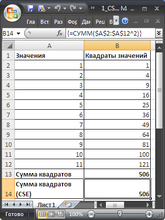
В отличие от ввода обычных формул, после ввода формулы массива нужно нажать вместо ENTER комбинацию клавиш CTRL+SHIFT+ENTER (поэтому, иногда, формулы массива также называются формулами CSE — это первые буквы от названия клавиш, используемых для ввода C trl, S hift, E nter). После этого формула будет обрамлена в фигурные скобки < >(их не вводят с клавиатуры, они автоматически появляются после нажатия CTRL+SHIFT+ENTER ). Это обрамление показано на рисунке выше (см. Строку формул ).
Если бы мы нажали просто ENTER , то получили бы сообщение об ошибке #ЗНАЧ!, возникающую при использовании неверного типа аргумента функции, т.к. функция СУММ() принимает в качестве аргумента только диапазон ячеек (или формулу, результатом вычисления которой является диапазон, или константы). В нашем случае мы в качестве аргумента ввели не диапазон, а некое выражение, которое еще нужно вычислить перед суммированием, поэтому и получили ошибку.
Чтобы глубже понять формулы массива проведем эксперимент:
- выделим ячейку B13 , содержащую обычную формулу =СУММ($B$2:$B$12) ;
- в C троке формул выделим аргумент функции СУММ() , т.е. $B$2:$B$12 ;
- нажмем клавишу F9 , т.е. вычислим, выделенную часть формулы;
- получим <1:4:9:16:25:36:49:64:81:100:121>– массив квадратов значений из столбца В . Массив – это просто набор неких элементов (значений).
Т.е. обычная функция СУММ() в качестве аргумента получила некий массив (или точнее ссылку на него).Теперь проведем тот же эксперимент с формулой массива:
- выделим ячейку, содержащую формулу массива =СУММ($A$2:$A$12^2) ;
- в строке формул выделим аргумент функции СУММ() , т.е. $A$2:$A$12^2 ;
- нажмем клавишу F9 , т.е. вычислим, выделенную часть формулы;
- получим <1:4:9:16:25:36:49:64:81:100:121>– тот же массив, что и в первом случае.
Т.е. нажатие CTRL+SHIFT+ENTER заставило EXCEL перед суммированием произвести промежуточные вычисления с диапазоном ячеек (с массивом содержащихся в нем значений). Для самой функции СУММ() ничего не изменилось – она получила тот же массив, только предварительно вычисленный, а не прямо из диапазона ячеек, как в случае с обычной формулой. Понятно, что вместо функции СУММ() в формуле массива может быть использована любая другая функция MS EXCEL: СРЗНАЧ() , МАКС() , НАИБОЛЬШИЙ() и т.п.
Вышеприведенный пример иллюстрирует использование функции массива возвращающей единственное значение, т.е. результат может быть выведен в одной ячейке. Это достигается использованием функций способных «свернуть» вычисленный массив до одного значения ( СУММ() , СРЗНАЧ() , МАКС() ). Примеры таких функций массива приведены в статье Формулы массива, возвращающие одно значение .
Формулы массива также могут возвращать сразу несколько значений. Понятно, что для того чтобы отобразить такой результат необходимо задействовать целый диапазон ячеек. Примеры таких функций приведены в статье Формулы массива, возвращающие несколько значений .
Преимущества и недостатки формул массива рассмотрены в одноименной статье Формулы массива. Преимущества и недостатки .
В файле примера также приведено решение данной задачи функцией СУММПРОИЗВ() , которая зачастую не требует введения ее как формулы массива: =СУММПРОИЗВ($A$2:$A$12^2)
Здесь, при вводе формулы СУММПРОИЗВ() нажимать CTRL+SHIFT+ENTER необязательно.
ПРИМЕЧАНИЕ : При создании Именованных формул и правил Условного форматирования формулы массива нельзя ввести нажимая CTRL+SHIFT+ENTER . Эти формулы вводятся только в ячейки листа. Однако, если формуле массива присвоить Имя , то EXCEL «сообразит», что нужно с ней нужно делать. Например, если формуле =СУММ($A$2:$A$12^2) присвоить имя Сумма_квадратов, а затем в ячейке указать =Сумма_квадратов , то получим правильный результат.
Источник
Ctrl Shift Войти в Excel — Выполнение расчетов по формулам массива

Ctrl Shift-Enter в Excel (Содержание)
- Объяснение Ctrl Shift-Enter в Excel
- Примеры Excel Control Shift-Enter
Excel Ctrl Shift-Enter
Ctrl Shift-Enter является одним из ярлыков, используемых в Excel для выполнения расчетов с формулами массива. Он поддерживает в выполнении сложных расчетов с использованием стандартных функций Excel. Он широко используется в формулах массива для применения функций и формул к набору данных. Совместное использование Ctrl Shift-Enter помогает конвертировать данные в формат массива, состоящий из нескольких значений данных в Excel. Он также поддерживает различие между обычной формулой и формулой массива. Благодаря этому ярлыку есть два основных преимущества, таких как работа с набором значений за раз, а также возврат нескольких значений за раз.
Объяснение Ctrl Shift-Enter в Excel
- Прежде чем использовать комбинацию клавиш CTRL SHIFT-ENTER, нам нужно больше узнать о массивах. Массивы — это набор данных, включающий текстовые и числовые значения в нескольких строках и столбцах или только в одной строке и столбце. Например, Array = (15, 25, -10, 24).
- Чтобы ввести вышеуказанные значения в массив, нам нужно ввести CTRL SHIFT + ENTER после выбора диапазона ячеек. В результате получается массив Array = (= (15, 25, -10, 24)).
- Как показано выше, фигурные скобки заключаются в формулу, приводя диапазон ячеек в одном горизонтальном массиве. Это сочетание клавиш работает в разных версиях Excel, включая 2007, 2010, 2013 и 2016 годы.
- CTRL SHIFT-ENTER также работает для вертикальных и многомерных массивов в Excel. Этот ярлык работает для различных функций, которые требуют использования данных в диапазоне ячеек. Он эффективно используется в различных операциях, таких как определение суммы и выполнение умножения матриц.
Как использовать Ctrl Shift-Enter в Excel?
CTRL SHIFT-ENTER используется во многих приложениях в Excel.
Вы можете скачать этот шаблон CTRL Shift-Enter Excel здесь — CTRL Shift-Enter Excel шаблон
- Создание формулы массива в матричных операциях, таких как умножение.
- Создание формулы массива при определении суммы множества значений.
- Замена сотен формул только одной формулой массива или суммирование диапазона данных, который соответствует определенным критериям или условиям.
- Подсчет количества символов или значений в диапазоне данных в Excel.
- Суммирование значений, представленных в каждом n-м столбце или строке в пределах нижней и верхней границ.
- Выполнение задачи по созданию простых наборов данных в короткие сроки.
- Расширение формулы массива до нескольких ячеек.
- Определение среднего, минимального, максимального, агрегированного и массива выражений.
- Возврат результатов в несколько ячеек с использованием формул массива.
- Использование CTRL SHIFT-ENTER в функциях IF.
Примеры Ctrl Shift-Enter в Excel
Ниже приведены примеры управления Excel Shift-Enter.
Пример № 1 — Определить сумму
Этот пример иллюстрирует использование Ctrl SHIFT-ENTER при расчете суммы продаж, созданных для разных продуктов. Следующие данные рассматриваются для этого примера.

Шаг 1: Поместите курсор в пустую ячейку, где вы хотите рассчитать общую сумму продаж продукта.

Шаг 2: введите формулу как сумма = сумма (D6: D11 * E6: E11), как показано на рисунке ниже.

Шаг 3: После ввода формулы нажмите CTRL SHIFT-ENTER, чтобы преобразовать общую формулу в формулу массива.

Шаг 4: Открывающая и закрывающая скобки добавляются в формулу суммы. Результат получается так, как показано на рисунке.

Шаг 5: Проверьте результат определения итога с помощью общей процедуры, которую мы использовали.

Результат, полученный в результате двух процедур, одинаков. Но использование формулы массива с помощью клавиши CTRL SHIFT ENTER позволяет легко определить общий объем продаж, исключив вычисление дополнительного столбца промежуточной суммы.
Пример №2. Определение суммы с использованием условия
Этот пример иллюстрирует использование Ctrl SHIFT-ENTER при расчете суммы продаж, сгенерированных для различных продуктов, с использованием условий. Следующие данные рассматриваются для этого примера.

Шаг 1: На первом шаге определите детали продавца и продукта, которые хотят рассчитать объем продаж, сгенерированный индивидуально. Рассмотрим продавца = John и Product = PC и введите эти данные в соответствующие ячейки, как показано на скриншоте ниже.

Шаг 2: Чтобы определить объем продаж, произведенных Джоном при продаже продуктов для ПК, формула
= СУММА (ЕСЛИ (((A2: A10 = F2) * (B2: B10 = F3)), (C2: C10)))

Шаг 3: Нажмите CTRL SHIFT-ENTER, чтобы получить желаемый результат, как показано на рисунке.

Шаг 4: Измените значения ячеек F2 и F3, чтобы определить продажи, произведенные другими лицами.

Таким образом, расчет сгенерированных продаж автоматизируется с помощью комбинации клавиш CTRL SHIFT-ENTER.
Пример № 3 — Определение обратной матрицы
Для этого примера рассмотрим следующую матрицу А.
Шаг 1: Введите матрицу A в лист Excel, как показано на рисунке ниже.

Диапазон матрицы B1: C2
Шаг 2: Выделите диапазон ячеек, чтобы расположить обратную матрицу A -1 на том же листе.

Шаг 3: После выделения диапазона ячеек введите формулу MINVERSE для вычисления обратной матрицы. Будьте внимательны при вводе формулы, чтобы все ячейки были выделены.

Шаг 4: Введите диапазон массива или матрицы, как показано на скриншоте.

Шаг 5: После успешного ввода функции MINVERSE используйте комбинацию клавиш CTRL SHIFT-ENTER, чтобы сгенерировать формулу массива, чтобы получить результаты всех четырех компонентов матрицы без повторного входа в другие компоненты. Преобразованная формула массива отображается как (= MINVERSE (B1: C2))

Шаг 6: Результирующая обратная матрица получается как:

То, что нужно запомнить
- Ручной ввод скобок вокруг формулы не работает в Excel. Мы должны нажать сочетание клавиш CTRL SHIFT-ENTER.
- Когда мы редактируем формулу массива, нам нужно снова нажать сочетание клавиш CTRL SHIFT-ENTER, поскольку скобки удаляются каждый раз, когда мы вносим изменения.
- При использовании ярлыка необходимо выбрать диапазон ячеек, чтобы получить результат, прежде чем вводить формулу массива.
Рекомендуемые статьи
Это руководство по нажатию клавиши CTRL-Enter в Excel. Здесь мы обсудим 3 способа использования Ctrl Shift-Enter в Excel для определения суммы, обратной матрицы и суммы с помощью условия, а также примеры и загружаемый шаблон Excel. Вы можете посмотреть наши следующие статьи, чтобы узнать больше —
- Как объединить ячейки с помощью ярлыков Excel?
- Что такое программирование в Excel?
- Ярлык для удаления строки в Excel
- Как закрасить альтернативные строки в Excel?
Источник
Ctrl Shift Enter in Excel


Excel Ctrl Shift-Enter Command
Ctrl Shift-Enter helps convert the data into an array format consisting of multiple data values in Excel. It also supports differentiation between the regular formula and array formula in excel Array Formula In Excel Array formulas are extremely helpful and powerful formulas that are used in Excel to execute some of the most complex calculations. There are two types of array formulas: one that returns a single result and the other that returns multiple results. read more . Using this shortcut provides two major advantages: dealing with a set of values and returning the multiple values simultaneously.
For example, we can calculate the sales and costs of various electronic gadgets over any given number of years.
Ctrl+Shift+Enter is one of the shortcuts used in Excel to perform the calculations with array formulas. It supports performing complex calculations using the standard excel functions Excel Functions Excel functions help the users to save time and maintain extensive worksheets. There are 100+ excel functions categorized as financial, logical, text, date and time, Lookup & Reference, Math, Statistical and Information functions. read more . It is widely used in the array formulae to apply functions and formulas to a data set.
Table of contents
Explanation
- Before we want to use the shortcut CTRL+SHIFT+ENTER, we need to understand more about the arrays. The array is the collection of the data, including text and numerical values in multiple rows and columns or only in a single row and column. For example, Array =
- To enter the above values into an array, we need to enter CTRL+SHIFT+ENTER after selecting the range of cells. It results in the array as:
- Array= <= <15, 25, -10, 24>>
- As shown above, braces are enclosed to the formula by resulting in the range of cells in a single horizontal array. This keyboard shortcutKeyboard ShortcutAn Excel shortcut is a technique of performing a manual task in a quicker way.read more works in different versions of Excel, including 2007, 2010, 2013, and 2016.
- CTRL+SHIFT+ENTER also works for vertical and multi-dimensional arrays in Excel. This shortcut works for different functions that require the use of data in a range of cells. It is effectively used in various operations like determining sums and performing matrix multiplication in excelMatrix Multiplication In ExcelThe MMULT function in Excel is an inbuilt function for matrix multiplication. It accepts two arrays as arguments and returns the product of the two arrays.read more .
You are free to use this image on your website, templates, etc., Please provide us with an attribution link How to Provide Attribution? Article Link to be Hyperlinked
For eg:
Source: Ctrl Shift Enter in Excel (wallstreetmojo.com)
Examples of Ctrl Shift-Enter In Excel
Example #1 – To Determine the Sum
This example best illustrates the use of Ctrl+SHIFT+ENTER in calculating the sum of sales generated for different products. Therefore, the following data is considered for this example.
Step 1: First, we must place the cursor into the empty cell where we want to produce the worth of the product’s total sales.
Step 2: As shown in the figure, we need to insert the formula as total = sum (D6:D11*E6: E11).
Step 3: After entering the formula, we must press CTRL+SHIFT +ENTER to convert the general formula into an array formula.
Step 5: Now, we need to check the result determining the total with the general procedure we used.
The result obtained from the two procedures is the same. But, using the array formula with CTRL+SHIFT+ENTER is easy to determine total sales by eliminating the calculation of an additional subtotal column.
Example #2 – To Determine Sum using Condition
This example best illustrates the use of Ctrl+SHIFT+ENTER in calculating the sum of sales generated for different products using the conditions. Therefore, the following data is considered for this example.
Step 1: In the first step, we need to determine the details of the seller and product that want to calculate sales generated individually. Consider Seller =John and Product = PC and enter these details into individual cells, as shown in the figure.
Step 2: To determine the sales generated by John in selling PC products, the formula as:
=SUM (IF (((A2:A10=F2)*(B2:B10=F3)), (C2:C10)))
Step 3: We mustpress CTRL+SHIFT+ENTER to have the desired result, as shown in the figure.
Step 4: Now, we need to change the values of F2 and F3 cells to determine sales generated by other persons.
In this way, the calculation of sales generated is automated using the shortcut CTRL+SHIFT+ENTER.
Example #3 – To Determine the Inverse Matrix
For this example, consider the following matrix A.
Follow the below steps to get the inverse matrix.
- Initially, we must enter the matrix A into the Excel sheet, as shown in the figure below.

The range of the matrix is B1:C2.
Then, highlight the range of cells to position the inverse matrix in Excel A-1 on the same sheet.

After highlighting the range of cells, we must input the formula of MINVERSE to calculate the inverse matrix.
Ensure during inputting the formula that all cells are highlighted.
First, we must enter the array or matrix range, as shown in the screenshot.
Once the MINVERSE function is entered successfully, we must use the shortcut CTRL+SHIFT+ENTER to generate the array formula to have the results of all four matrix components without re-entering to other details.
The converted array formula is shown as
<=MINVERSE (B1: C2)>
The resultant inverse matrix is produced as:

Applications
CTRL + SHIFT + ENTER is used in many applications in Excel.
- Creating an array formula in matrix operations such as multiplication.
- Creating an array formula in determining the sum of the set of values.
- Replacing the hundreds of formulas with only a single array formula or summing the range of data that meets specific criteria or conditions.
- To count the number of characters or values in the range of data in Excel.
- To sum the values presented in every nth column or row within low and upper boundaries.
- To perform the task of creating simple datasets in a short time.
- To expand the array formula to multiple cells.
- To determine the Average, Min, Max, Aggregate, and array expressions values.
- To return the results in multiple and single cells by applying the array formulas.
- To use CTRL+SHIFT+ENTER in the IF function in excelIF Function In ExcelIF function in Excel evaluates whether a given condition is met and returns a value depending on whether the result is “true” or “false”. It is a conditional function of Excel, which returns the result based on the fulfillment or non-fulfillment of the given criteria.read more .
Things to Remember
- The manual entering of braces surrounding the formula does not work in Excel. Instead, we should press the shortcut CTRL+SHIFT+ENTER.
- When we edit the array formula, we must press the shortcut CTRL+SHIFT+ENTER again since the braces are removed every time we change.
- Using the shortcut requires selecting the range of cells to result in the output before entering the array formula.
Recommended Articles
This article has been a guide to the Ctrl Shift-Enter in Excel. Here, we learn when and how to use Ctrl Shift-Enter in Excel, examples, and a downloadable template. You may learn more about Excel from the following articles: –
Источник
- Excel Ctrl Shift-Enter
Ctrl Shift-Enter в Excel (Содержание)
- Объяснение Ctrl Shift-Enter в Excel
- Примеры Excel Control Shift-Enter
Excel Ctrl Shift-Enter
Ctrl Shift-Enter является одним из ярлыков, используемых в Excel для выполнения расчетов с формулами массива. Он поддерживает в выполнении сложных расчетов с использованием стандартных функций Excel. Он широко используется в формулах массива для применения функций и формул к набору данных. Совместное использование Ctrl Shift-Enter помогает конвертировать данные в формат массива, состоящий из нескольких значений данных в Excel. Он также поддерживает различие между обычной формулой и формулой массива. Благодаря этому ярлыку есть два основных преимущества, таких как работа с набором значений за раз, а также возврат нескольких значений за раз.
Объяснение Ctrl Shift-Enter в Excel
- Прежде чем использовать комбинацию клавиш CTRL SHIFT-ENTER, нам нужно больше узнать о массивах. Массивы — это набор данных, включающий текстовые и числовые значения в нескольких строках и столбцах или только в одной строке и столбце. Например, Array = (15, 25, -10, 24).
- Чтобы ввести вышеуказанные значения в массив, нам нужно ввести CTRL SHIFT + ENTER после выбора диапазона ячеек. В результате получается массив Array = (= (15, 25, -10, 24)).
- Как показано выше, фигурные скобки заключаются в формулу, приводя диапазон ячеек в одном горизонтальном массиве. Это сочетание клавиш работает в разных версиях Excel, включая 2007, 2010, 2013 и 2016 годы.
- CTRL SHIFT-ENTER также работает для вертикальных и многомерных массивов в Excel. Этот ярлык работает для различных функций, которые требуют использования данных в диапазоне ячеек. Он эффективно используется в различных операциях, таких как определение суммы и выполнение умножения матриц.
Как использовать Ctrl Shift-Enter в Excel?
CTRL SHIFT-ENTER используется во многих приложениях в Excel.
Вы можете скачать этот шаблон CTRL Shift-Enter Excel здесь — CTRL Shift-Enter Excel шаблон
- Создание формулы массива в матричных операциях, таких как умножение.
- Создание формулы массива при определении суммы множества значений.
- Замена сотен формул только одной формулой массива или суммирование диапазона данных, который соответствует определенным критериям или условиям.
- Подсчет количества символов или значений в диапазоне данных в Excel.
- Суммирование значений, представленных в каждом n-м столбце или строке в пределах нижней и верхней границ.
- Выполнение задачи по созданию простых наборов данных в короткие сроки.
- Расширение формулы массива до нескольких ячеек.
- Определение среднего, минимального, максимального, агрегированного и массива выражений.
- Возврат результатов в несколько ячеек с использованием формул массива.
- Использование CTRL SHIFT-ENTER в функциях IF.
Примеры Ctrl Shift-Enter в Excel
Ниже приведены примеры управления Excel Shift-Enter.
Пример № 1 — Определить сумму
Этот пример иллюстрирует использование Ctrl SHIFT-ENTER при расчете суммы продаж, созданных для разных продуктов. Следующие данные рассматриваются для этого примера.
Шаг 1: Поместите курсор в пустую ячейку, где вы хотите рассчитать общую сумму продаж продукта.
Шаг 2: введите формулу как сумма = сумма (D6: D11 * E6: E11), как показано на рисунке ниже.
Шаг 3: После ввода формулы нажмите CTRL SHIFT-ENTER, чтобы преобразовать общую формулу в формулу массива.
Шаг 4: Открывающая и закрывающая скобки добавляются в формулу суммы. Результат получается так, как показано на рисунке.
Шаг 5: Проверьте результат определения итога с помощью общей процедуры, которую мы использовали.
Результат, полученный в результате двух процедур, одинаков. Но использование формулы массива с помощью клавиши CTRL SHIFT ENTER позволяет легко определить общий объем продаж, исключив вычисление дополнительного столбца промежуточной суммы.
Пример №2. Определение суммы с использованием условия
Этот пример иллюстрирует использование Ctrl SHIFT-ENTER при расчете суммы продаж, сгенерированных для различных продуктов, с использованием условий. Следующие данные рассматриваются для этого примера.
Шаг 1: На первом шаге определите детали продавца и продукта, которые хотят рассчитать объем продаж, сгенерированный индивидуально. Рассмотрим продавца = John и Product = PC и введите эти данные в соответствующие ячейки, как показано на скриншоте ниже.
Шаг 2: Чтобы определить объем продаж, произведенных Джоном при продаже продуктов для ПК, формула
= СУММА (ЕСЛИ (((A2: A10 = F2) * (B2: B10 = F3)), (C2: C10)))
Шаг 3: Нажмите CTRL SHIFT-ENTER, чтобы получить желаемый результат, как показано на рисунке.
Шаг 4: Измените значения ячеек F2 и F3, чтобы определить продажи, произведенные другими лицами.
Таким образом, расчет сгенерированных продаж автоматизируется с помощью комбинации клавиш CTRL SHIFT-ENTER.
Пример № 3 — Определение обратной матрицы
Для этого примера рассмотрим следующую матрицу А.
Пусть А = 10 8
4 6
Шаг 1: Введите матрицу A в лист Excel, как показано на рисунке ниже.
Диапазон матрицы B1: C2
Шаг 2: Выделите диапазон ячеек, чтобы расположить обратную матрицу A -1 на том же листе.
Шаг 3: После выделения диапазона ячеек введите формулу MINVERSE для вычисления обратной матрицы. Будьте внимательны при вводе формулы, чтобы все ячейки были выделены.
Шаг 4: Введите диапазон массива или матрицы, как показано на скриншоте.
Шаг 5: После успешного ввода функции MINVERSE используйте комбинацию клавиш CTRL SHIFT-ENTER, чтобы сгенерировать формулу массива, чтобы получить результаты всех четырех компонентов матрицы без повторного входа в другие компоненты. Преобразованная формула массива отображается как (= MINVERSE (B1: C2))

Шаг 6: Результирующая обратная матрица получается как:

То, что нужно запомнить
- Ручной ввод скобок вокруг формулы не работает в Excel. Мы должны нажать сочетание клавиш CTRL SHIFT-ENTER.
- Когда мы редактируем формулу массива, нам нужно снова нажать сочетание клавиш CTRL SHIFT-ENTER, поскольку скобки удаляются каждый раз, когда мы вносим изменения.
- При использовании ярлыка необходимо выбрать диапазон ячеек, чтобы получить результат, прежде чем вводить формулу массива.
Рекомендуемые статьи
Это руководство по нажатию клавиши CTRL-Enter в Excel. Здесь мы обсудим 3 способа использования Ctrl Shift-Enter в Excel для определения суммы, обратной матрицы и суммы с помощью условия, а также примеры и загружаемый шаблон Excel. Вы можете посмотреть наши следующие статьи, чтобы узнать больше —
- Как объединить ячейки с помощью ярлыков Excel?
- Что такое программирование в Excel?
- Ярлык для удаления строки в Excel
- Как закрасить альтернативные строки в Excel?