
X out a cell in Excel
There are a couple ways to cross out a cell in Excel. My favorite way is shown first, but a more manual option is also shown right after the first. Both methods are outlined below.
Method 1 (my favorite way to cross out a cell): Add a Small Tool – Make Excel Better
You can add a tool into Excel that will make it super easy to cross out cells. Or if a cell is crossed out, uncross it out. You can use the tool to set the line color, set the thickness of the line, and choose between a solid line or a dotted line for the “X”.
Or, you can right-click the highlighted cells and select Cross Out Cell(s) from the context menu.
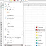
You get these same menu options with the tool if you right-click in a cell. The menus fly out as you hover and make your selection.
The tool also also adds a feature to unhide all the hidden tabs. When you’re done looking at them you can re-hide them with a single click. As with the cross-out tool, you can right-click on a worksheet tab and you will have the unhide all and re-hide sheets available to you there too.
The added functionality makes it much quicker to cross out cells or to toggle hidden worksheet tabs on and off in Excel. There is no trial version of the basic OPU Workbook Tools for Excel add-in. However, there is a trial version of the Excel Powerups Premium Suite which includes the OPU Workbook Tools functionality. You can get that trial version from the Download link at the top of this page.
Method 2: Manually Format the Cell
You can easily X out a cell in Excel by manually placing an X from corner to corner in a cell in Excel. Follow the steps below with the accompanying screen shots.
- Select the cell(s) you wish to place the X’s.
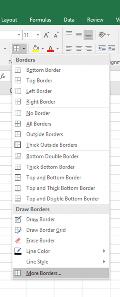
- From the Borders drop down menu in the Font section on the Home tab, select More Borders at the bottom of the menu.
- The Format Cells dialog box appears. In the Format Cells dialog box, select the Border tab.
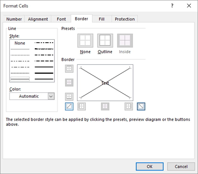
- Select both of the corner line buttons. There is one on either of the lower right and left corners of the big box in the center of the dialog box.

and

- Click OK.
You can change the color of the X by changing the color of the lines used. Just change the selection in the Color drop down box from Automatic to the color you prefer.
If you want to uncross out the cell you can go back to the same Borders drop down list. On that list there is an option for No Borders. However, if you have any other borders (for example, you’re doing this in a table) selecting the No Border option will get rid of the table borders on any cells you’ve selected.
Alternatively, you can go back to the More Borders dialog box and unselect each of the diagonal corner line buttons.
So you can see if you have to do this more than once, it’s really not that feasible to do manually all the time. That’s why I use the OPU Workbook Tools for Excel tool mentioned above.
Also bundled into EPPS, you may already have OPU Workbook Tools for Excel
If you already have the Excel PowerUps Premium Suite, you already have the Cross Out tool. With a cell or range of cells selected you click the Cross Out Cell(s) button in the OPU Workbook Tools section of the PowerUps ribbon or in the context menu just as in the best method outlined above.
If you don’t see it in your current version, you can get the most recent version from https://officepowerups.com/update.
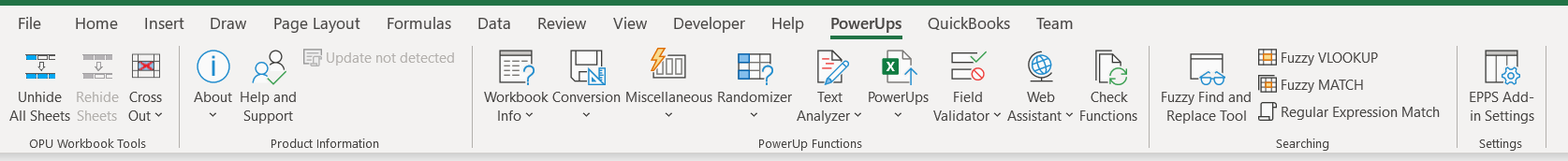
Table of Contents
- INTRODUCTION
- WHAT IS CROSSING OUT OR STRIKE THROUGH TEXT IN EXCEL?
- WHEN IS CROSS OUT USED IN EXCEL ?
- WAYS TO CROSS OUT TEXT IN EXCEL
- CROSS OUT TEXT IN EXCEL USING RIGHT CLICK OPTION
- CROSS OUT TEXT IN EXCEL USING EXCEL RIBBON OPTION
- CROSS OUT TEXT IN EXCEL USING KEYBOARD SHORTCUT
- REMOVE CROSS OUT FORMAT FROM TEXT IN EXCEL
- CROSS OUT ONLY A PART OF THE TEXT WITHIN A CELL
INTRODUCTION
Crossing out the text is needed many times while making the reports.
CROSSING OUT TEXT PLACES A HORIZONTAL LINE THROUGH THE TEXT.
The formatting of the text consists of many operations such as setting the size of the text or numbers, making them bold for giving emphasis,
underlining them for showing the importance and
Crossing out needed to show some values which are important to be shown but removed from the list
So, in this article we would learn various fast and speedy ways to strike through the text in excel.
WHAT IS CROSSING OUT OR STRIKE THROUGH TEXT IN EXCEL?
CROSSING OUT OR STRIKE THROUGH simply means to put a horizontal line through the word.
Cross out or strike through or strike out means cancelling a word or nullifying something which was already present.
WHEN IS CROSS OUT USED IN EXCEL ?
CROSSING OUT THE TEXT to show that
- Something which has been removed from the data.
- Any task which was there but now has been completed.
- Anything , where we want to show the presence of some information but which has been omitted or has become redundant.
For the example,
Suppose, we have a list of chores
- Do the dishes.
- Wash the car.
- Go to Market.
- Meet any friend and so on.
After we have complete two jobs. Our list can be shown as
Do the dishes.- Wash the car.
- Go to Market.
- Meet any friend and so on.
CROSS OUT, STRIKE THROUGH, STRIKE OUT , ALL THESE WORDS MEANS THE SAME. IT MEANS THE STRIKE THROUGH TEXT
WAYS TO CROSS OUT TEXT IN EXCEL
We can use many ways to strike through the text in Excel.
The ways available are :
- RIGHT CLICK > FORMAT CELLS.
- EXCEL RIBBON
- KEYBOARD SHORTCUT
Let us discuss all the ways one by one in detail.
CROSS OUT TEXT IN EXCEL USING RIGHT CLICK OPTION
This section deals with the techniques to CROSS OUT the text in Excel.
STEPS TO CROSSOUT THE TEXT IN EXCEL.
- Right Click the cell containing the text which needs to be crossed out and choose FORMAT CELLS.

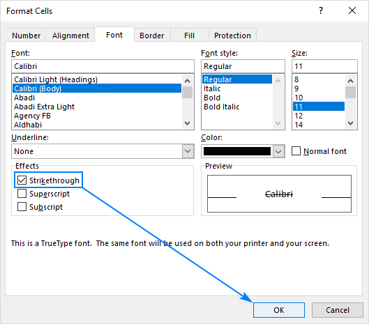
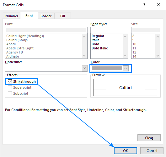
- In the dialog box opened, go to FONT TAB and click STRIKETHROUGH as shown in the picture below.

- Click OK.
- The text will be CROSSED OUT.
Look at the final picture.

CROSS OUT TEXT IN EXCEL USING EXCEL RIBBON OPTION
We can also strikethrough our text directly from the EXCEL RIBBON.
STEPS TO CROSS OUT USING THE OPTION PRESENT IN EXCEL RIBBON:
- Select the cell in which you want to strikethrough the text.
- Click the FONT SETTINGS button on the EXCEL RIBBON. Location is shown below in the picture.

- After clicking FONT SETTINGS button, again the FORMAT CELLS DIALOG BOX will open.
- Check the STRIKETHROUGH option.
- Click OK.
- The text in the selected cell will start showing the Strikethrough format.

- Click OK.
- The text will be striked through.
The final text looks like this one.

CROSS OUT TEXT IN EXCEL USING KEYBOARD SHORTCUT
The fastest way of operation in any software is still the use of KEYBOARD SHORTCUTS.
We are lucky to have a keyboard shortcut for the use of STRIKETHROUGH too.
Follow the steps to use keyboard shortcut to CROSS OUT any text in Excel.
- Select the cell in which we want to strikethrough the text.
- Press CTRL , and press 5.
- It’ll strikethrough the text within fractions of seconds.
- After clicking FONT SETTINGS button, again the FORMAT CELLS DIALOG BOX will open.
- Check the STRIKETHROUGH option.
- Click OK.
- The text in the selected cell will start showing the CROSS OUT format.
REMOVE CROSS OUT FORMAT FROM TEXT IN EXCEL
STRIKETHROUGH is a toggle function [ When keyboard shortcut is used ].
TOGGLE FUNCTIONS WORK IN AN ON OFF WAY.
Once used, they’ll put the effect on, pressed again they’ll remove the effect. Simply select the cell or text and click CTRL+5. [ 5 on the main keyboard and not on the numeric pad]
Strikethrough will be removed.Similarly, we can easily remove strikethrough by
- Select the cells from which you want to remove Strikethrough.
- Open FONT SETTINGS WINDOW or RIGHT CLICK > FORMAT CELL.
- Deselect STRIKETHROUGH and click OK.
- CROSSED OUT FORMAT will be reversed.
CROSS OUT ONLY A PART OF THE TEXT WITHIN A CELL
Some students ask this questions whether we can CROSS OUT a part of the text in a single cell .
The answer is YES!!
Strikethrough option to cross out would work only on the part of the text which you have selected before applying the operation.
It means, if you want to cross out a portion of a text, simply select it and use any of the above mentioned methods to StrikeThrough the selected text easily.Look at the animation below.
These were a few ways to strike out or cross out text in Excel.
Apply or Remove Strikethrough Using Shortcuts in Excel
by Avantix Learning Team | Updated July 20, 2021
Applies to: Microsoft® Excel® 2013, 2016, 2019 and 365 (Windows)
You can apply strikethrough to text or values in Excel to cross out or create a line through a cell or part of a cell. There are 3 common ways to apply strikethrough in your Excel worksheets – using a built-in keyboard shortcut, using the Format Cells dialog box, or by adding a command to the Quick Access Toolbar.
Recommended article: How to Delete Blank Rows in Excel (5 Easy Ways)
Do you want to learn more about Excel? Check out our virtual classroom or live classroom Excel courses >
What is strikethrough?
Strikethrough is a character format that can be applied to text or values in a cell where a line appears through the cell or selected text. Because it’s a format, it can be removed easily. If you double-click in a cell, you can drag over the text or values and apply strikethrough.
Applying strikethrough using a built-in keyboard shortcut
To apply strikethrough to a cell using a built-in keyboard shortcut:
- Select the cell you want to strikethrough.
- Press Ctrl + 5.
If you double-click in a cell and then highlight text or partial text in a cell, you can still use this shortcut. Press Ctrl + 5 if you want to remove strikethrough as well.
Applying strikethrough using the Format Cells dialog box
To apply strikethrough to a cell or the contents of a cell using the Format Cells dialog box and keyboard shortcuts:
- Select the cell you want to strikethrough. You can also double-click in a cell and drag over partial text.
- Press Ctrl + Shift + F. The Format Cells dialog box appears with the Font tab selected.
- Press Alt + K to select Strikethrough (note that k is the underlined letter).
- Press Enter.
Below is the Format Cells dialog box in Excel with Strikethrough selected:

Adding Strikethrough to the Quick Access Toolbar
Another strategy is to add Strikethrough to the Quick Access Toolbar and then access it using Alt.
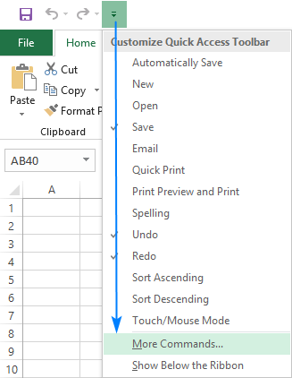
It’s typically easier to work with the Quick Access Toolbar if you display it below the Ribbon. If the Quick Access Toolbar is above the Ribbon, click the down arrow to the right of the Quick Access Toolbar and select Show Below the Ribbon from the drop-down menu.
To add Strikethrough to the Quick Access Toolbar in Excel:
- Click the down arrow to the right of the Quick Access Toolbar and select More commands from the drop-down menu. The Options dialog box appears.
- Below Choose command from, select All Commands from the drop-down menu.
- In the list of commands, click Strikethrough and then click Add.
- In the list of commands below Customize Quick Access Toolbar, click Strikethrough.
- Click the up arrow that appears on the far right until the button appears at the top of the list (you can move it to the second position, third position, etc.).
- Click OK.
- Press Alt. Key tips appear on the Quick Access Toolbar. If you have moved Strikethrough to the first position, press 1 to apply it. If you have moved Strikethrough to the second position, press 2 to apply it and so on. These are sequential shortcuts, so press Alt and then the number.
Below is the Options dialog box in Excel and Strikethrough has been added on the right:

You can also simply click the Strikethrough command on the Quick Access Toolbar to apply or remove it.
Subscribe to get more articles like this one
Did you find this article helpful? If you would like to receive new articles, join our email list.
More resources
How to Merge Cells in Excel (4 Ways)
How to Remove Duplicates in Excel (3 Easy Ways)
How to Use Flash Fill in Excel (4 Ways with Shortcuts)
How to Combine Cells in Excel using Concatenate (3 Ways)
How to Replace Blank Cells with a Value from the Cell Above in Excel
Related courses
Microsoft Excel: Intermediate / Advanced
Microsoft Excel: Data Analysis with Functions, Dashboards and What-If Analysis Tools
Microsoft Excel: Introduction to Power Query to Get and Transform Data
Microsoft Excel: New and Essential Features and Functions in Excel 365
Microsoft Excel: Introduction to Visual Basic for Applications (VBA)
VIEW MORE COURSES >
Our instructor-led courses are delivered in virtual classroom format or at our downtown Toronto location at 18 King Street East, Suite 1400, Toronto, Ontario, Canada (some in-person classroom courses may also be delivered at an alternate downtown Toronto location). Contact us at info@avantixlearning.ca if you’d like to arrange custom instructor-led virtual classroom or onsite training on a date that’s convenient for you.
Copyright 2023 Avantix® Learning
Microsoft, the Microsoft logo, Microsoft Office and related Microsoft applications and logos are registered trademarks of Microsoft Corporation in Canada, US and other countries. All other trademarks are the property of the registered owners.
Avantix Learning |18 King Street East, Suite 1400, Toronto, Ontario, Canada M5C 1C4 | Contact us at info@avantixlearning.ca
Содержание
- How to strikethrough in Excel
- How to strikethrough in Excel
- Excel strikethrough shortcut
- Apply strikethrough via cell format options
- Add a strikethrough button to Quick Access Toolbar
- Put a strikethrough button onto Excel ribbon
- How to strikethrough automatically with conditional formatting
- Add strikethrough with a macro
- How to use strikethrough in Excel Online
- How to strikethrough in Excel for Mac
- How to remove strikethrough in Excel
- Remove strikethrough added manually
- Remove strikethrough added with conditional formatting
- How to Insert Cross Text Symbol in Excel & Google Sheets
- Inserting the Cross Text Symbol into Excel
- Inserting a Cross Symbol Using the Wingdings Font and the Alt Code
- Inserting a Cross Mark Using the Wingdings 2 Font
- Inserting the Cross Text Symbol into Google Sheets
- Inserting a Cross Symbol Using the CHAR Function
- Inserting a Cross Symbol Using Special Characters
How to strikethrough in Excel
 by Svetlana Cheusheva, updated on March 17, 2023
This short tutorial explains different ways to add, use and remove strikethrough format in Excel desktop, Excel Online and Excel for Mac.
Excel is great for manipulating numbers, but it does not always make clear how to format text values the way you want. Strikethrough is a vivid example.
It is super easy to cross out text in Microsoft Word — you simply click the strikethrough button on the ribbon. Naturally, you’d expect to see the same button on the Excel ribbon. But it’s nowhere to be found. So, how do I strikethrough text in Excel? By using any of the six methods described in this tutorial 🙂
How to strikethrough in Excel
To ensure that everyone is on the same page, let’s define the term first. What does it mean to strikethrough in Excel? Simply, to put a line through a value in a cell. There are a handful of different ways to do this, and we are going to begin with the fastest one.
Excel strikethrough shortcut
Want to have the job done as quickly as possible? Press a hotkey or key combination.
Here’s the keyboard shortcut to strikethrough in Excel: Ctrl + 5
The shortcut can be used on an entire cell, certain part of the cell contents, or a range of cells.
To apply the strikethrough format to a cell, select that cell, and press the shortcut: 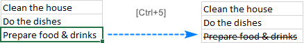
To draw a line through all values in a range, select the range: 
To strikethrough non-adjacent cells, select multiple cells while holding the Ctrl key, and then press the strikethrough shortcut: 
To cross out part of the cell value, double-click the cell to enter the Edit mode, and select the text you want to strikethrough: 
Apply strikethrough via cell format options
Another quick way to draw a line through a cell value in Excel is by using the Format Cells dialog. Here’s how:
- Select one or more cells on which you want to apply the strikethrough format.
- Press Ctrl + 1 or right-click the selected cell(s) and choose Format Cells… from the context menu.
- In the Format Cells dialog box, go to the Font tab, and tick off the Strikethrough option under Effects.
- Click OK to save the change and close the dialog.
Add a strikethrough button to Quick Access Toolbar
If you think that the above method requires too many steps, add the strikethrough button to the Quick Access Toolbar to always have it at your fingertips.
- Click the small arrow in the upper left corner of the Excel window, and then click More Commands…

- Under Choose commands from, select Commands Not in the Ribbon, then select Strikethrough in the list of commands, and click the Add button. This will add Strikethrough to the list of commands on the right pane, and you click OK:
Look at the upper left corner of your worksheet again, and you will find the new button there:
Put a strikethrough button onto Excel ribbon
If your Quick Access Toolbar is reserved only for the most frequently used commands, which strikethrough is not, place it onto the ribbon instead. As with QAT, it’s also one-time setup, performed in this way:
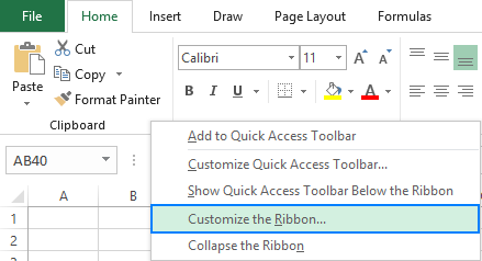
- Right-click anywhere on the ribbon and select Customize the Ribbon… from the pop-up menu:
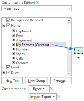
- Since new buttons can only be added to custom groups, let’s create one. For this, select the target tab (Home in our case) and click the New Group button. Then, click Rename… to name the newly created group to your liking, say My Formats:
- With the new group selected, perform the already familiar steps: under Choose commands from, select Commands Not in the Ribbon, find Strikethrough in the list of commands, select it, and click Add:
- Click OK to save the changes, and find the Strikethrough button on your Excel ribbon:

You can now cross out text in Excel with a single button click! And it will also remind you the keyboard shortcut in case you forget it 🙂
Tip. By using Up and Down arrows in the Excel Options dialog box, you can move your custom group with the Strikethrough button to any position on the ribbon:
How to strikethrough automatically with conditional formatting
In case you are planning to use a strikethrough to cross out the completed tasks or activities in a checklist or to-do list, you may want Excel to do it for you automatically as you enter some text in a related cell, for example «done»: 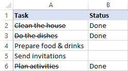
The task can be easily accomplished with Excel Conditional Formatting:
- Select all the cells you want to cross out on condition (A2:A6 in this example).
- On the Home tab, in the Styles group, click Conditional Formatting >New Rule…
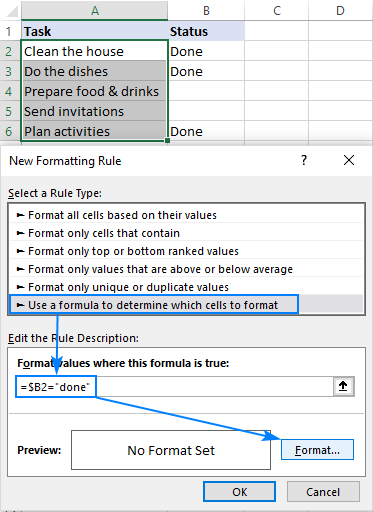
- In the New Formatting Rule dialog box, select Use a formula to determine which cells to format.
- In the Format values where this formula is true box, enter the formula that expresses the condition for your topmost cell:
=$B2=»Done»

Instead of defining a task status with text, you can insert checkboxes, link them to some cells (which you can hide later) and base your conditional formatting rule on the value in the linked cells (TRUE is a checkbox is checked, FALSE if not checked).
As the result, Excel will check off the completed tasks automatically depending on whether the checkbox is selected or not. 
If you’d like to create something similar in your worksheets, the detailed steps can be found here: How to create a checklist with conditional formatting.
Add strikethrough with a macro
If you are not allergic to using VBA in your Excel worksheets, you can apply strikethrough on all selected cells with this line of code:
The step-by-step instructions on how to insert VBA code in Excel can be found here.
How to use strikethrough in Excel Online
In Excel Online, the strikethrough option is exactly where you’d expect to find it — next to the other formatting buttons on the Home tab, in the Font group: 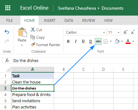
However, there’s a fly in the ointment — it’s not possible to select non-adjacent cells or ranges in Excel Online. So, if you need to cross out multiple entries in different parts of your sheet, you will have to select each cell or a range of contiguous cells individually, and then click the strikethrough button.
The strikethrough shortcut ( Ctrl + 5 ) works perfectly in Excel Online too and is often the fastest way to toggle the strikethrough formatting on and off.
In case you are interested, you can learn more about how to move your worksheets in Excel Online.
How to strikethrough in Excel for Mac
A quick way to strikethrough text in Excel for Mac is by using this keyboard shortcut: ⌘ + SHIFT + X 
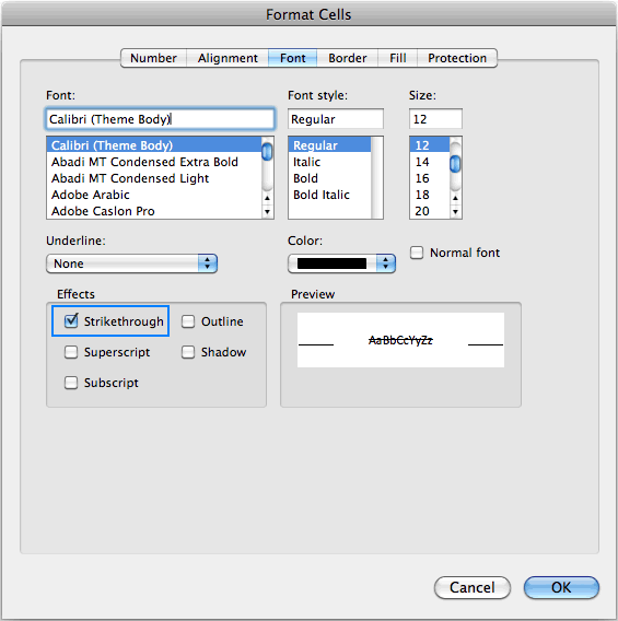
It can also be done from the Format Cells dialog in the same way as in Excel for Windows:
- Select the cell(s) or part of a cell value you wish to cross out.
- Right-click the selection and chose Format Cells from the popup menu.
- In the Format Cells dialog box, switch to the Font tab and select the Strikethrough checkbox:
How to remove strikethrough in Excel
The correct way to remove strikethrough from a cell depends on how you’ve added it.
Remove strikethrough added manually
If you applied strikethrough via a shortcut or cell format, then press Ctrl + 5 again, and the formatting will be gone.
A longer way would be opening the Format Cells dialog ( Ctrl + 1 ) and unchecking the Strikethrough box there: 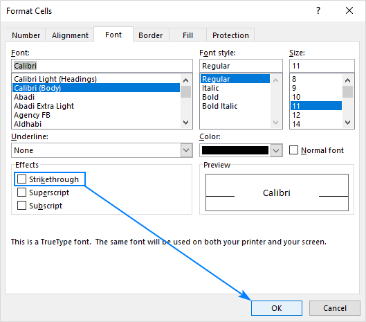
Remove strikethrough added with conditional formatting
If strikethrough is added by a conditional formatting rule, then you need to remove that rule to get rid of strikethrough.
To have it done, select all the cells from which you want to remove strikethrough, go to the Home tab > В Styles group, and click Conditional Formatting > Clear Rules > Clear Rules from Selected Cells: 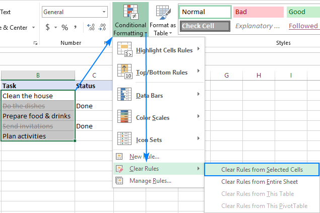
If some other conditional formatting rule(s) is applied to the same cells and you’d like to keep that rule, then click conditional Formatting > Manage Rules… and delete only the strikethrough rule.
That’s how you can add and remove the strikethrough formatting in Excel. I thank you for reading and hope to see you on our blog next week!
Источник
How to Insert Cross Text Symbol in Excel & Google Sheets
This tutorial will demonstrate how to insert a cross text symbol into Excel and Google Sheets.
Inserting the Cross Text Symbol into Excel
Excel has a few options for inserting bullet points. The first is to use the Symbols feature.
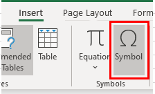
1. In the Ribbon, select Insert > Symbols > Symbol.
2. The Symbol box will appear. You can resize the box if you wish so see more symbols by dragging the bottom right-hand corner of the box.
3. Change the font in the left-hand drop-down box to “Wingdings”.
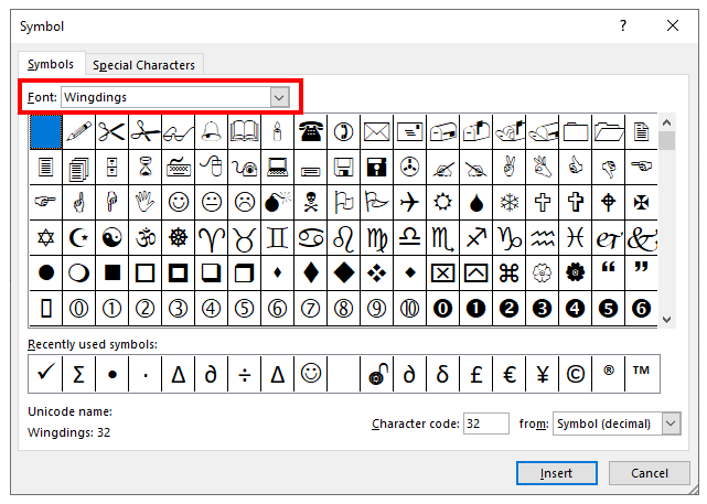
4. Scroll down until you find the cross symbol and click on Insert.
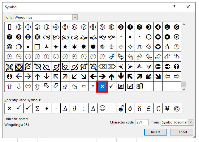
5. Click Close to return to Excel.
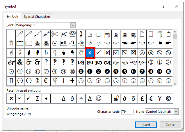
You can also amend the font to Wingdings 2 and find the cross symbol in that character set.
Inserting a Cross Symbol Using the Wingdings Font and the Alt Code
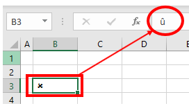
We can also insert a cross symbol into Excel by changing the font to Wingdings in the Excel screen and typing the character û directly into a cell.
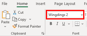
1. In the Ribbon, select Home > Font and then select Wingdings from the Font drop-down box.
2. Hold down the Alt key, and then type ALT + 0251.
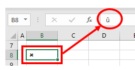
3. The character û is inserted into Excel. The Wingdings font will display this character as a cross mark.
Inserting a Cross Mark Using the Wingdings 2 Font
In the Ribbon, select Home > Font and then select Wingdings 2 from the Font drop-down box.
In the selected cell, hold down the shift key and press the letter O (uppercase O).
Inserting the Cross Text Symbol into Google Sheets
Inserting a Cross Symbol Using the CHAR Function
We can insert cross symbols into Google Sheets by using the CHAR Function.
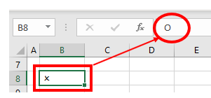
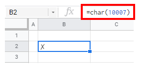
Select the cell you wish to insert your cross text symbol into and type in the CHAR Function with the relevant number (for example: 10007).
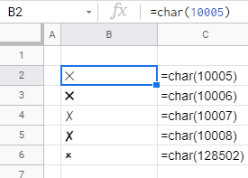
Using the numbers 10005, 10006, 1008, and 128502 with the CHAR Function will show slightly different cross marks.
Inserting a Cross Symbol Using Special Characters
Google Sheets does not have a symbol function. Google Documents, however, does. If you wish to insert symbols such as the cross mark into Google sheets you need to open a Google document and copy and paste from that document into the Google sheet.
1. In the File menu, select New > Document.
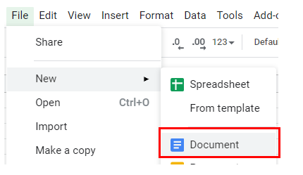
A new tab will open in the browser showing a new Google document.
2. In the Insert Menu, select Special characters.
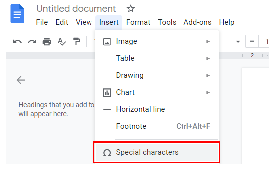
We are able to select a variety of categories in the left drop-down box such as Symbol, Emoji, Punctuation etc.
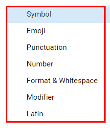
3. Select Symbol in the left-hand drop-down box, and then select Miscellaneous in the right-hand box.
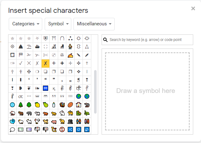
4. Click on the Ballot or Ballot Heavy symbol to insert the symbol into the Google document.
5. Click the close button to close the Special Characters box.
6. Highlight the symbol with your mouse and then press CTRL + C to copy the symbol.
7. Switch back to the Google sheet and press CTRL + V to paste the symbol.
Источник