Cross table in excel - Word и Excel - помощь в работе с программами

A crosstab is a table that summarizes the relationship between two categorical variables.

The following step-by-step example explains how to create a crosstab in Excel.

Step 1: Enter the Data

First, let’s enter the following dataset into Excel:

Step 2: Create the Crosstab

Next, click the Insert tab along the top ribbon and then click the PivotTable button.

In the new window that appears, select the range that contains the data as the Table/Range and choose any cell you’d like in the Existing Worksheet to place the crosstab. We’ll choose cell E2:

Step 3: Populate the Crosstab with Values

Once you click OK, a new window on the right side of the screen will appear.

Drag the Team variable to the Rows area, the Position variable to the Columns area, then the Position variable again to the Values area as follows:

Once you do so, the following crosstab will appear in the cell that you specified:

Step 4: Interpret the Crosstab

Here’s how to interpret the values in the crosstab:

Row Totals:

A total of 6 players are on team A
A total of 6 players are on team B

Column Totals:

A total of 3 players have a position of Center
A total of 4 players have a position of Forward
A total of 5 players have a position of Guard

Individual Cells:

1 player has a position of Center on team A
3 players have a position of Forward on team A
2 players have a position of Guard on team A
2 players have a position of Center on team B
1 player has a position of Forward on team B
3 players have a position of Guard on team B

Additional Resources

The following tutorials offer additional information on how to calculate frequencies in Excel:

How to Calculate Relative Frequency in Excel
How to Calculate Cumulative Frequency in Excel
How to Create a Frequency Polygon in Excel

Источник

17 авг. 2022 г.
читать 2 мин

Кросс -таблица — это таблица, которая обобщает взаимосвязь между двумя категориальными переменными.

В следующем пошаговом примере объясняется, как создать кросс-таблицу в Excel.

Шаг 1: введите данные

Во-первых, давайте введем следующий набор данных в Excel:

Шаг 2: Создайте кросс-таблицу

Затем щелкните вкладку « Вставка » на верхней ленте, а затем нажмите кнопку « Сводная таблица ».

В появившемся новом окне выберите диапазон, содержащий данные, в качестве таблицы/диапазона , а затем выберите любую ячейку на существующем рабочем листе для размещения кросс-таблицы. Мы выберем ячейку E2 :

Шаг 3. Заполните кросс-таблицу значениями

После того, как вы нажмете OK, появится новое окно в правой части экрана.

Перетащите переменную Team в область Rows , переменную Position в область Columns , затем снова переменную Position в область Values следующим образом:

После этого в указанной ячейке появится следующая кросс-таблица:

Шаг 4. Интерпретация кросс-таблицы

Вот как интерпретировать значения в кросс-таблице:

Всего строк:

Всего в команде А 6 игроков.
Всего в команде B 6 игроков.

Итоги столбца:

Всего 3 игрока занимают позицию центра.
Всего 4 игрока имеют позицию Forward
Всего 5 игроков имеют позицию Стража.

Отдельные ячейки:

1 игрок занимает позицию центра в команде А
3 игрока имеют позицию нападающего в команде А
2 игрока занимают позицию Guard в команде A
2 игрока занимают позицию центра в команде B
1 игрок имеет позицию нападающего в команде B
3 игрока имеют позицию Guard в команде B

Дополнительные ресурсы

В следующих руководствах представлена дополнительная информация о том, как вычислять частоты в Excel:

Как рассчитать относительную частоту в Excel
Как рассчитать кумулятивную частоту в Excel
Как создать полигон частот в Excel

Написано

Замечательно! Вы успешно подписались.

Добро пожаловать обратно! Вы успешно вошли

Вы успешно подписались на кодкамп.

Срок действия вашей ссылки истек.

Ура! Проверьте свою электронную почту на наличие волшебной ссылки для входа.

Успех! Ваша платежная информация обновлена.

Ваша платежная информация не была обновлена.

Источник

Have you ever used VLOOKUP to bring a column from one table into another table? Now that Excel has a built-in Data Model, VLOOKUP is obsolete. You can create a relationship between two tables of data, based on matching data in each table. Then you can create Power View sheets and build PivotTables and other reports with fields from each table, even when the tables are from different sources. For example, if you have customer sales data, you might want to import and relate time intelligence data to analyze sales patterns by year and month.

All the tables in a workbook are listed in the PivotTable and Power View Fields lists.

When you import related tables from a relational database, Excel can often create those relationships in the Data Model it’s building behind the scenes. For all other cases, you’ll need to create relationships manually.

Make sure the workbook contains at least two tables, and that each table has a column that can be mapped to a column in another table.
Do one of the following: Format the data as a table, or Import external data as a table in a new worksheet.
Give each table a meaningful name: In Table Tools, click Design > Table Name > enter a name.
Verify the column in one of the tables has unique data values with no duplicates. Excel can only create the relationship if one column contains unique values.

For example, to relate customer sales with time intelligence, both tables must include dates in the same format (for example, 1/1/2012), and at least one table (time intelligence) lists each date just once within the column.
Click Data > Relationships.

If Relationships is grayed out, your workbook contains only one table.

In the Manage Relationships box, click New.
In the Create Relationship box, click the arrow for Table, and select a table from the list. In a one-to-many relationship, this table should be on the many side. Using our customer and time intelligence example, you would choose the customer sales table first, because many sales are likely to occur on any given day.
For Column (Foreign), select the column that contains the data that is related to Related Column (Primary). For example, if you had a date column in both tables, you would choose that column now.
For Related Table, select a table that has at least one column of data that is related to the table you just selected for Table.
For Related Column (Primary), select a column that has unique values that match the values in the column you selected for Column.
Click OK.

More about relationships between tables in Excel

Notes about relationships
Example: Relating time intelligence data to airline flight data
“Relationships between tables may be needed”
- Step 1: Determine which tables to specify in the relationship
- Step 2: Find columns that can be used to create a path from one table to the next

Notes about relationships

You’ll know whether a relationship exists when you drag fields from different tables onto the PivotTable Fields list. If you aren’t prompted to create a relationship, Excel already has the relationship information it needs to relate the data.
Creating relationships is similar to using VLOOKUPs: you need columns containing matching data so that Excel can cross-reference rows in one table with those of another table. In the time intelligence example, the Customer table would need to have date values that also exist in a time intelligence table.
In a data model, table relationships can be one-to-one (each passenger has one boarding pass) or one-to-many (each flight has many passengers), but not many-to-many. Many-to-many relationships result in circular dependency errors, such as “A circular dependency was detected.” This error will occur if you make a direct connection between two tables that are many-to-many, or indirect connections (a chain of table relationships that are one-to-many within each relationship, but many-to-many when viewed end to end. Read more about Relationships between tables in a Data Model.
The data types in the two columns must be compatible. See Data types in Excel Data Models for details.
Other ways to create relationships might be more intuitive, especially if you are not sure which columns to use. See Create a relationship in Diagram View in Power Pivot.

Example: Relating time intelligence data to airline flight data

You can learn about both table relationships and time intelligence using free data on the Microsoft Azure Marketplace. Some of these datasets are very large, requiring a fast internet connection to complete the data download in a reasonable period of time.

Start Power Pivot in Microsoft Excel add-in and open the Power Pivot window.
Click Get External Data > From Data Service > From Microsoft Azure Marketplace. The Microsoft Azure Marketplace home page opens in the Table Import Wizard.
Under Price, click Free.
Under Category, click Science & Statistics.
Find DateStream and click Subscribe.
Enter your Microsoft account and click Sign in. A preview of the data should appear in the window.
Scroll to the bottom and click Select Query.
Click Next.
Choose BasicCalendarUS and then click Finish to import the data. Over a fast internet connection, import should take about a minute. When finished, you should see a status report of 73,414 rows transferred. Click Close.
Click Get External Data > From Data Service > From Microsoft Azure Marketplace to import a second dataset.
Under Type, click Data.
Under Price, click Free.
Find US Air Carrier Flight Delays and click Select.
Scroll to the bottom and click Select Query.
Click Next.
Click Finish to import the data. Over a fast internet connection, this can take 15 minutes to import. When finished, you should see a status report of 2,427,284 rows transferred. Click Close. You should now have two tables in the data model. To relate them, we’ll need compatible columns in each table.
Notice that the DateKey in BasicCalendarUS is in the format 1/1/2012 12:00:00 AM. The On_Time_Performance table also has a datetime column, FlightDate, whose values are specified in the same format: 1/1/2012 12:00:00 AM. The two columns contain matching data, of the same data type, and at least one of the columns (DateKey) contains only unique values. In the next several steps, you’ll use these columns to relate the tables.
In the Power Pivot window, click PivotTable to create a PivotTable in a new or existing worksheet.
In the Field List, expand On_Time_Performance and click ArrDelayMinutes to add it to the Values area. In the PivotTable, you should see the total amount of time flights were delayed, as measured in minutes.
Expand BasicCalendarUS and click MonthInCalendar to add it to the Rows area.
Notice that the PivotTable now lists months, but the sum total of minutes is the same for every month. Repeating, identical values indicate a relationship is needed.
In the Field List, in “Relationships between tables may be needed”, click Create.
In Related Table, select On_Time_Performance and in Related Column (Primary) choose FlightDate.
In Table, select BasicCalendarUS and in Column (Foreign) choose DateKey. Click OK to create the relationship.
Notice that the sum of minutes delayed now varies for each month.
In BasicCalendarUS and drag YearKey to the Rows area, above MonthInCalendar.

You can now slice arrival delays by year and month, or other values in the calendar.

Tips: By default, months are listed in alphabetical order. Using the Power Pivot add-in, you can change the sort so that months appear in chronological order.

Make sure that the BasicCalendarUS table is open in the Power Pivot window.
On the Home table, click Sort by Column.
In Sort, choose MonthInCalendar
In By, choose MonthOfYear.

The PivotTable now sorts each month-year combination (October 2011, November 2011) by the month number within a year (10, 11). Changing the sort order is easy because the DateStream feed provides all of the necessary columns to make this scenario work. If you’re using a different time intelligence table, your step will be different.

“Relationships between tables may be needed”

As you add fields to a PivotTable, you’ll be informed if a table relationship is required to make sense of the fields you selected in the PivotTable.

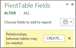
Although Excel can tell you when a relationship is needed, it can’t tell you which tables and columns to use, or whether a table relationship is even possible. Try following these steps to get the answers you need.

Step 1: Determine which tables to specify in the relationship

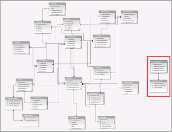
If your model contains just a few tables, it might be immediately obvious which ones you need to use. But for larger models, you could probably use some help. One approach is to use Diagram View in the Power Pivot add-in. Diagram View provides a visual representation of all the tables in the Data Model. Using Diagram View, you can quickly determine which tables are separate from the rest of the model.

Note: It’s possible to create ambiguous relationships that are invalid when used in a PivotTable or Power View report. Suppose all of your tables are related in some way to other tables in the model, but when you try to combine fields from different tables, you get the “Relationships between tables may be needed” message. The most likely cause is that you’ve run into a many-to-many relationship. If you follow the chain of table relationships that connect to the tables you want to use, you will probably discover that you have two or more one-to-many table relationships. There is no easy workaround that works for every situation, but you might try creating calculated columns to consolidate the columns you want to use into one table.

Step 2: Find columns that can be used to create a path from one table to the next

After you’ve identified which table is disconnected from the rest of the model, review its columns to determine whether another column, elsewhere in the model, contains matching values.

For example, suppose you have a model that contains product sales by territory, and that you subsequently import demographic data to find out if there is correlation between sales and demographic trends in each territory. Because the demographic data comes from a different data source, its tables are initially isolated from the rest of the model. To integrate the demographic data with the rest of your model, you’ll need to find a column in one of the demographic tables that corresponds to one you’re already using. For example if the demographic data is organized by region, and your sales data specifies which region the sale occurred, you could relate the two datasets by finding a common column, such as a State, Zip code, or Region, to provide the lookup.

Besides matching values, there are a few additional requirements for creating a relationship:

Data values in the lookup column must be unique. In other words, the column can’t contain duplicates. In a Data Model, nulls and empty strings are equivalent to a blank, which is a distinct data value. This means that you can’t have multiple nulls in the lookup column.
Data types of both the source column and lookup column must be compatible. For more information about data types, see Data types in Data Models.

To learn more about table relationships, see Relationships between tables in a Data Model.

Top of Page

Источник

Hristina Hristova

Course Author

This Cross Table in Excel shows how a typical cross-table can be constructed. The rows of the table represent the type of investment while the investors are placed as columns. Each cell, therefore, shows how much each person invested and where. Some other related topics you might be interested to explore are Side-by-side bar chart in Excel, Bar chart in Excel, Pie chart in Excel, Histogram in Excel, Frequency Distribution Table for Numerical Variables.
You can now download the Excel template for free.
Cross Table in Excel is among the topics covered in detail in the 365 Data Science program.

Who is it for

This is an open-access Excel template in .xlsx format that will be useful for Data Analysts, Data Scientists, Business Analysts, and everyone who works with Excel to visualize data.

How it can help you

The following template puts you in the shoes of an investment manager, managing stocks, bonds and real estate investments for 3 different investors. You will learn how to create a cross-table containing information about the allocations of each investor, as well as the total investments either by type of investment, or by investor.

Источник

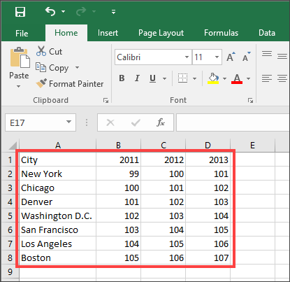
Excel is a very useful tool in data analysis, and it’s always a good thing to master as many skills as you can to save time and effort at work. One common question is: how can I convert a cross table (a.k.a. two-dimensional table) to a flat list (a.k.a. one-dimensional list) in Excel? Although flat list is the ideal form for analyzing, the data we get in daily life usually appear as cross tables so it’s necessary to know how to do the conversion.

If you’re not familiar with cross tables and flat lists, here’s what they look like:

Cross Table/Two-dimensional Table: a common form to record data

Flat List/One-dimensional List: the ideal form for data analysis

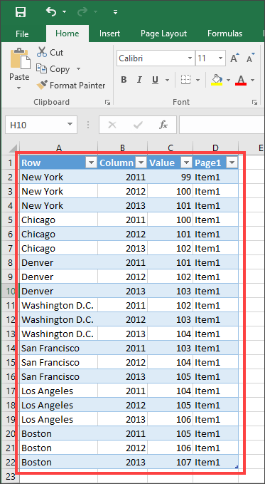
Can you find out the difference between these two forms? In the lower list, you can see that the metric for year (shown as the first row in the upper cross table) has been converted to a single column, which means it’s no longer a metric but a list of data.

How to convert a cross table to a flat list

To convert a cross table to a flat list, you can perform the following procedure:

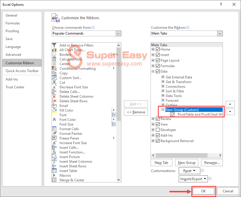
If you already have the PivotTable and PivotChart Wizard function on your top menu, you can skip Step 1 – 3 and head straight to Step 4.

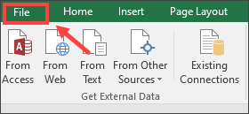
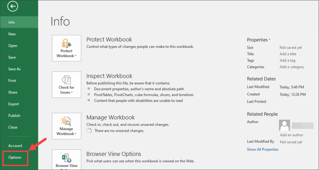
1) In the top menu, select File.

Then click Options in the left pane.

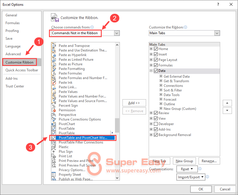
2) In the left pane, select Customize Ribbon; on the right panel, under Choose commands from, select Commands Not in the Ribbon, and find PivotTable and PivotChart Wizard in the list below.

3) Expand the Data category and click New Group. When the New Group (Custom) item is created, click to highlight PivotTable and PivotChart Wizard in the left list and click Add >>. Now the PivotTable and PivotChart Wizard function should’ve been added to Data > New Group (Custom).

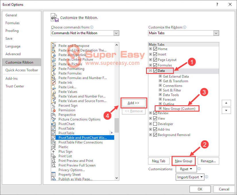
When complete, don’t forget to click OK to save the changes.

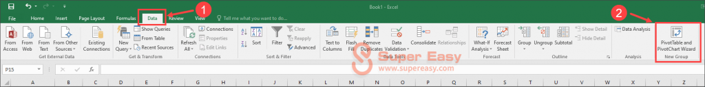
4) Go back to the Excel window, and click PivotTable and PivotChart Wizard on the Data tab.

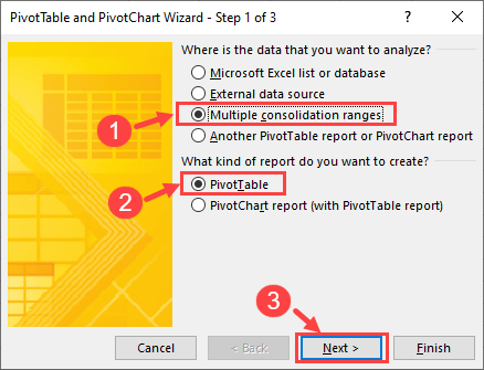
5) In the pop-up window, select Multiple consolidation ranges and PivotTable. Then, click Next >.

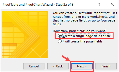
6) Click Next >.

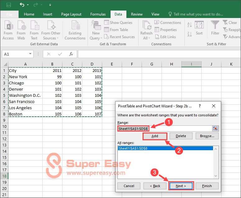
7) Under Range:, select all the data you need and click Add. If you succeed, the range you selected should appear in the All ranges section. Once complete, click Next >.

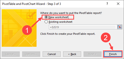
Select New worksheet and then click Finish.

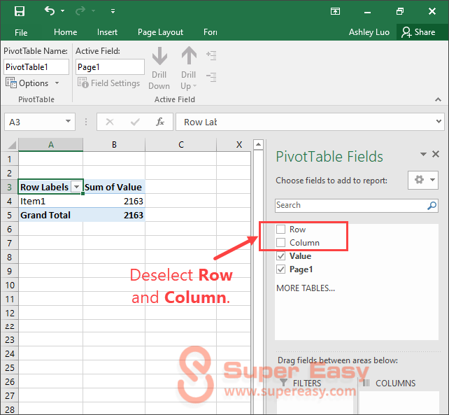
9) In the new PivotTable, deselect the Row and Column options.

10) Double-click the number next to Grand Total.

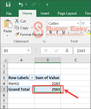
11) There you go! A one-dimensional list should be created in a new sheet.

So this is the end of this short tutorial. Hopefully it helped you solve your problem! If you have any further questions or ideas, please feel free to leave a comment below.

Extra Info:

Want to get a leg up in your career?

Try Udacity – an e-learning platform for tech-focused learners!

It’s never been too late for you to learn new tech skills. No matter if it’s about programming, data analysis, or other fields. All you need is a little passion, a little perseverance, and a little professional guidance. Udacity will do the last part for you.

For any penny-wise learners, Driver Easy Coupons provides the latest deals, coupons, and promo codes that actually work. Before heading to the checkout, why not have a look at the coupon page for Udacity and save yourself a few bucks?

What If the Promo Code Doesn’t Work?

Ensure you’ve entered the promo code and your purchase meets all restrictions, such as minimum spend, regional-use, new customers only, etc. If the code still doesn’t work, it could be an expired or inaccurate coupon. While our goal is to provide only valid coupons, unfortunately, we can’t guarantee that once in a while a non-working or expired coupon will appear on our website.

Be sure to confirm any coupon has been applied before you complete your purchase.

Ashley loves to write about pets, games, snacks and everything she’s interested in. She’s a big fan of RPG games including Skyrim, Witcher 3, Dragon Age, Mass Effect and so on. Knowing her way around money-saving tips and life hacks, she’s always ready to help people save big on purchases. She also works as a tech writer at drivereasy.com.

Contributor(s):

Источник

Содержание

How To Create A Cross Tabulation In Excel?
What is a cross tabulation called in Excel?
Which of the following can be used to quickly create cross tabulations?
Is cross tabulation Chi Square?
Which tabulation is all example of cross tabulation?
How do you make a contingency table?
What kind of variables would you cross tabulate?
How do you explain a cross tabulation table?
How do I enable filtering in Excel?
How do you use Simmons crosstab?
What is a Crosstab banner?
How do I report crosstabs results?
What is the difference between crosstabs and Chi Square?
How does a crosstabs with chi square analysis function?
Is Chi square and crosstab the same?
Is cross-tabulation descriptive statistics?
How many variables can a cross-tabulation include?
What does a contingency table look like?
How do you do a chi-square goodness of fit test in Excel?
What is chi square test example?
Cross-tab or contingency table in Excel
Dataset to create a cross-tab or contingency table
Creating a cross-tab or contingency table
Results of the creation of a cross-tab or contingency table
Statistical tests on cross-tabs or contingency tables
Advantages of using XLSTAT cross-tabs instead of Excel pivot tables

How To Create A Cross Tabulation In Excel?

What is a cross tabulation called in Excel?

Cross tabulation is a method to quantitatively analyze the relationship between multiple variables. Also known as contingency tables or cross tabs, cross tabulation groups variables to understand the correlation between different variables.

Which of the following can be used to quickly create cross tabulations?

PivotTables can be used to quickly create cross-tabulations and to drill down into a large set of data in numerous ways.

Is cross tabulation Chi Square?

Crosstabulation is a powerful technique that helps you to describe the relationships between categorical (nominal or ordinal) variables.

Which tabulation is all example of cross tabulation?

Cross tabulation is a statistical tool that is used to analyze categorical data. Categorical data is data or variables that are separated into different categories that are mutually exclusive from one another. An example of categorical data is eye color.

How do you make a contingency table?

Creating a basic contingency table. To create a contingency table of the data in the var1 column cross-classified with the data in the var2 column, choose the Stat > Tables > Contingency > With Data menu option. Select var1 as the Row variable, choose var2 as the Column variable, and click Compute!.

What kind of variables would you cross tabulate?

You typically use cross tabulation when you have categorical variables or data – e.g. information that can be divided into mutually exclusive groups. For example, a categorical variable could be customer reviews by region.

How do you explain a cross tabulation table?

Cross tabulations are simply data tables that present the results of the entire group of respondents as well as results from sub-groups of survey respondents. Cross tabulations enable you to examine relationships within the data that might not be readily apparent when analyzing total survey responses.

How do I enable filtering in Excel?

Try it!

Select any cell within the range.
Select Data > Filter.
Select the column header arrow .
Select Text Filters or Number Filters, and then select a comparison, like Between.
Enter the filter criteria and select OK.

How do you use Simmons crosstab?

Step-by-Step: How to Create a Cross Tab

Enter Search Terms. Simmons has a “smart search” feature.
Create rows or columns. Add variables to either columns or rows by clicking the appropriate button after you have identified your variable(s).
Create Rows.
Run the Cross Tab.
View your Cross Tab.
Export Your Work.

A crosstabulation (or “crosstab”) is a table displaying survey results. It resembles a spreadsheet with multiple rows and columns, typically where the rows are tabulated survey responses and the columns are subgroups for analysis.

How do I report crosstabs results?

Setup

Go to Results > Reports.
Click Create Report > Crosstab.
Give your report a Title.
Add Your Columns, also know as Banners.
Next, add your Rows (aka Stubs).
Finally, choose from the below crosstab options and click Add Crosstab when you are finished.
Frequencies – These are just the counts of responses.

What is the difference between crosstabs and Chi Square?

Cross tabulation table (also known as contingency or crosstab table) is generated for each distinct value of a layer variable (optional) and contains counts and percentages. Chi-square test is used to check if the results of a cross tabulation are statistically significant.

How does a crosstabs with chi square analysis function?

A cross tabulation displays the joint frequency of data values based on two or more categorical variables. The joint frequency data can be analyzed with the chi-square statistic to evaluate whether the variables are associated or independent.This table shows frequency counts for each production line and shift.

Is Chi square and crosstab the same?

Crosstabulation is a statistical technique used to display a breakdown of the data by these two variables (that is, it is a table that has displays the frequency of different majors broken down by gender). The Pearson chi-square test essentially tells us whether the results of a crosstab are statistically significant.

Is cross-tabulation descriptive statistics?

Descriptive Statistics.Descriptive Statistics includes the tools shown on the left. These are typical tools for exploring the descriptive summaries, frequencies, and cross-tabulation tables. These exploring tools along with graphical tools are not only useful for data exploration, but also are useful for data cleaning

How many variables can a cross-tabulation include?

two variables
A cross-tabulation (or just crosstab) is a table that looks at the distribution of two variables simultaneously.

What does a contingency table look like?

A contingency table usually shows frequencies for particular combinations of values of two discrete random variable s X and Y. Each cell in the table represents a mutually exclusive combination of X-Y values. This is a two-way 2×3 contingency table (i.e. two rows and three columns).

How do you do a chi-square goodness of fit test in Excel?

Chi Square Goodness of Fit Test Help

Enter the data into an Excel worksheet as shown below. The data can be downloaded at this link.
Select all the data in the table above including the headings.
Select “Misc.
Select the “Chi Square Goodness of Fit” option and then OK.

What is chi square test example?

Chi-Square Independence Test – What Is It? if two categorical variables are related in some population. Example: a scientist wants to know if education level and marital status are related for all people in some country. He collects data on a simple random sample of n = 300 people, part of which are shown below.

Источник

Cross-tab or contingency table in Excel

This tutorial shows how to create a cross-tab, also called contingency table from two qualitative variables in Excel using the XLSTAT software.

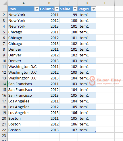
Dataset to create a cross-tab or contingency table

The dataset contains information on 20 clients: their age, city of residence and gender. We will create a contingency table based on the Age and City variables.

Creating a cross-tab or contingency table

After opening XLSTAT, select the XLSTAT / Preparing data / Create a contingency table command.

Once you’ve clicked on the relevant button, the dialog box appears.

In the General tab, select the category variable you wish to use in rows. Select the Age variable by selecting the entire column. Then select the variable to be used in columns. Here we choose the City variable. The columns B and C contain variable labels so the option Variable labels should be ticked.

You may activate the By group analysis field if you want to use a layer variable, such as the gender, and generate a three-way cross-tab.

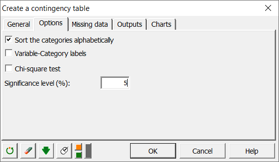
In the Options tab, you can decide how the categories of the variable should be treated. Also you can choose to run a Chi-square test. In this case, however, we will only select the Sort the categories alphabetically option.

In the Outputs tab, select the Contingency table as well as the observed and theoritical frequencies.

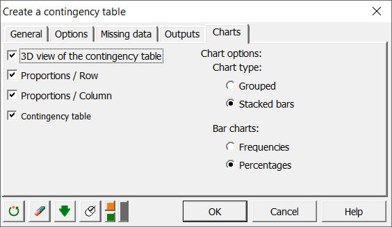
Select the following options in the tab Charts.

The computations begin once you have clicked on the OK button, and the results are displayed on a new sheet.

Results of the creation of a cross-tab or contingency table

The first result is the contingency table. Notice that clients are absent in certain crossed categories. For example there is no detected client in Paris of age class 25-34.

The next output is the 3-D plot followed by a stacked bar chart, which is a good visualization of the data distribution.

Next are the two tables containing the frequencies Age/City. You can compare the actual distribution of the clients and the theoritical distribution if the distribution was random.

Statistical tests on cross-tabs or contingency tables

It is possible to test if the two qualitative variables that shape the contingency table are independent.

Advantages of using XLSTAT cross-tabs instead of Excel pivot tables

Among the many advantages of using the XLSTAT contingency table feature compared to Excel pivot tables: — XLSTAT is able to automatically output test results on the contingency tables.

You can enter as many qualitative variables as you want in both the row and column variable fields in XLSTAT. XLSTAT will produce one result for each possible pair of row/column variables.

The following video tackles crosstabs with an illustration using XLSTAT:

Источник

This tutorial shows how to create a cross-tab, also called contingency table from two qualitative variables in Excel using the XLSTAT software.

Dataset to create a cross-tab or contingency table

The dataset contains information on 20 clients: their age, city of residence and gender. We will create a contingency table based on the Age and City variables.

Creating a cross-tab or contingency table

After opening XLSTAT, select the XLSTAT / Preparing data / Create a contingency table command.

Once you’ve clicked on the relevant button, the dialog box appears.

You may activate the By group analysis field if you want to use a layer variable, such as the gender, and generate a three-way cross-tab.

In the Outputs tab, select the Contingency table as well as the observed and theoritical frequencies.

Select the following options in the tab Charts.

The computations begin once you have clicked on the OK button, and the results are displayed on a new sheet.

Results of the creation of a cross-tab or contingency table

The first result is the contingency table. Notice that clients are absent in certain crossed categories. For example there is no detected client in Paris of age class 25-34.

The next output is the 3-D plot followed by a stacked bar chart, which is a good visualization of the data distribution.

Next are the two tables containing the frequencies Age/City. You can compare the actual distribution of the clients and the theoritical distribution if the distribution was random.

Statistical tests on cross-tabs or contingency tables

It is possible to test if the two qualitative variables that shape the contingency table are independent.

Advantages of using XLSTAT cross-tabs instead of Excel pivot tables

Among the many advantages of using the XLSTAT contingency table feature compared to Excel pivot tables: — XLSTAT is able to automatically output test results on the contingency tables.

You can enter as many qualitative variables as you want in both the row and column variable fields in XLSTAT. XLSTAT will produce one result for each possible pair of row/column variables.

The following video tackles crosstabs with an illustration using XLSTAT:

Was this article useful?

Источник

Put your cursor anywhere in your table then use Data>Get & Transform Data>From Table/Range. If you have an earlier version of Excel, this may be accessible via the Power Query Add-In.

The Power Query Editor should open and show you this:

Select Col2 by clicking the header and use Home>Transform>Group By, like this:

When you click OK, you will see that Summing Col1 causes an Error:

Use Home>Query>Advanced Editor, so that you see this:

Now change the part that says this:

List.Sum([Col1])

To this:

Text.Combine([Col1],", ")

So that you have this:

let
    Source = Excel.CurrentWorkbook(){[Name="Table1"]}[Content],
    #"Changed Type" = Table.TransformColumnTypes(Source,{{"Col1", type text}, {"Col2", Int64.Type}}),
    #"Grouped Rows" = Table.Group(#"Changed Type", {"Col2"}, {{"Col1", each Text.Combine([Col1],", "), type text}})
in
    #"Grouped Rows"

When you click OK you will get the results you want:

Now you can use Home>Close & Load to load the results into your workbook. When new data are added to the source table, just right-click the table in the workbook and choose «Refresh» to run the transformation again.

Источник