
Updated 12/16/2022: Stay up to date on the latest from Excel and download Excel templates today.
If you want to look up a value in a table using one criterion, it’s simple. You can use a plain VLOOKUP formula. But if you want to use more than one criterion, what can you do? There are lots of ways to use several Microsoft Excel functions such as VLOOKUP, LOOKUP, MATCH, and INDEX. In this blog post, I’ll show you a few of those ways.

Get a better picture of your data.
Using two criteria to return a value from a table
Let’s look at a scenario where you want to use two criteria to return a value. Here’s the data you have:

The criteria are “Name” and “Product,” and you want them to return a “Qty” value in cell C18. Because the value that you want to return is a number, you can use a simple SUMPRODUCT() formula to look for the Name “James Atkinson” and the Product “Milk Pack” to return the Qty. The SUMPRODUCT formula in cell C18 looks like this:
=SUMPRODUCT((B3:B13=C16)*(C3:C13=C17)*(D3:D13))
What it does is look in the range B3:B13 for the value in cell C16, and in the range C3:C13 for the value in cell C17. When it finds both, it returns the value in column D, from the same row where it met both criteria. Here’s how it will look:

It returns the value 1, which corresponds to the value in cell D4 (“James Atkinson” in row 4 and also “Milk Pack” in the same row), thus returning the value in column D from that row. Let’s change the value in cell C5 from “Wine Bottle” to “Milk Pack” to see what happens with the formula in cell C18:

Because our formula found two lines where both criteria were met, it sums the values in column D in both rows, giving us a Qty of 6.
This technique cannot be used if you want to look for two criteria and return a text result. For instance, this, would not work:

You would be looking for the Name “James Atkinson” where the Qty is 1, and you’d like to return the Product name that matches these two criteria. This formula would give us a #VALUE error! Instead, you could use a formula using a combination of SUMPRODUCT, INDEX, and ROW functions, such as this one:
=INDEX(C3:C13,SUMPRODUCT((B3:B13=C16)*(D3:D13=C18)*ROW(C3:C13)),0)
You use the SUMPRODUCT function to find out the row where both criteria are met, and return the corresponding row number using the ROW function. Then you use SUMPRODUCT in the INDEX function to return the value in the array C3:C13 that is in the row number provided. The result will be like this:
Using Lookup and multivalued fields in queries
Learn more

You could also do this using a different technique, such as this formula in cell C17:
=LOOKUP(2,1/(B3:B13=C16)/(D3:D13=C18),(C3:C13))
The result will be the same as in the previous solution. What this formula does, is divide 1 by an array of True/False values (B3:B13=C16), and then by another array of True/False values (D3:D13=C18). This will return either 1 or a #DIV/0! error. If you use 2 as the lookup value, then the formula will match it with the last numeric value in the range, that is, the last row where both conditions are True. This is the “vector form” of the LOOKUP, so you can use it to get the corresponding value returned from C3:C13. I used 2 as the LOOKUP value, but it can be any number, starting at 1. If the formulas don’t find any match, you will, of course, get a #N/A error!
You could also use an array formula, using the MATCH function, like this:
{=INDEX(C3:C13,MATCH(1,(B3:B13=C16)*(D3:D13=C18),0))}
With this technique, you can use the MATCH function to find the row where both conditions are met. This returns a value of 1, which is matched to the 1 that is used as the lookup value of the MATCH function, thus returning us to the row where the conditions are met. Using the INDEX value, you can look for the value that is in the range C3:C13, which is in the row that was returned from the MATCH function. In this case, it was row 2, which corresponds to the second row in the range C3:C13.

Task management in Microsoft 365
Collaborate on shared Office documents, including Excel, Word, and PowerPoint.
Using multiple criteria to return a value from a table
All of these examples show you how to use two criteria for lookups. It’s also easy to use these formulas if you have more than two criteria-you just add them to the formulas. Here is how the formulas would look if you add one more criterion:
=SUMPRODUCT((B3:B13=C16)*(C3:C13=C17)*(E3:E13=C18)*(D3:D13))
=INDEX(C3:C13,SUMPRODUCT((B3:B13=C16)*(D3:D13=C18)*(E3:E13=C18)*ROW(C3:C13)),0)
=LOOKUP(2,1/(B3:B13=C16)/(D3:D13=C18)/(E3:E13=C18),(C3:C13))
{=INDEX(C3:C13,MATCH(1,(B3:B13=C16)*(D3:D13=C18)*(E3:E13=C18),0))}
Learn more
As you can see, depending on what’s in your data tables, you can use several different techniques using different Excel functions to look up values. Enjoy applying these to your own Excel spreadsheets.
How to Use INDEX MATCH
With Multiple Criteria in Excel
INDEX MATCH with multiple criteria enables you to do a successful lookup when there are multiple lookup value matches.
In other words, you can look up and return values even if there are no unique values to look for.
This is not achievable with any other lookup formula without inserting helper columns😲
Follow these 3 easy steps to create your very own INDEX MATCH with multiple criteria in a few minutes.
If you want to tag along, download the sample Excel file here.
INDEX MATCH with multiple criteria example
So, you got this employee database.

You want to make the database easier to search, so you’re creating a small tool (to the right).
In that tool, anyone should be able to type in the name and division of an employee and it will find that person’s salary (and show it in cell G4).
“That’s easy, I can just use VLOOKUP.”
Wait a minute✋
Unfortunately, it’s not that easy.
You see, the problem is that there are actually 2 employees called “Steve Jones”. That means the lookup value has 2 matches in the lookup column.

There’s nothing unique about Steve Jones’ name on its own.
In Excel terminology, ‘Name’ would be 1 criteria.
So, 1 criteria didn’t cut it.
But if you include another criteria, like ‘Division’, you make Steve Jones unique.

Now, while “Steve Jones” appears several times on the list, there’s only one “Steve Jones from the sales division”.
This is the kind of magic you can do with INDEX MATCH with multiple criteria.
Step 1: Insert a normal INDEX MATCH formula
INDEX MATCH with multiple criteria is an ‘array formula’ created from the INDEX and MATCH functions.
An array formula has a syntax that is different from normal formulas. It’s basically a normal formula on steroids💪
The synergies between the INDEX and MATCH functions are that:
- MATCH searches for a value and returns a location
- MATCH feeds the location to the INDEX function
- Then INDEX transforms this location into a result

Start with:
=MATCH(
1. As the first argument in the MATCH function, enter the lookup value. This is what you are looking for.
In this case, you’re looking for an employee with the name “Steve Jones”.
Select (or manually enter) cell G2 as lookup value, then separate with a comma to move on to the lookup array.

2. The lookup array is the column where the MATCH function looks for the lookup value.
Select the column with the names, and then enter a comma to move on to the [match_type].

Now your formula should look like this:
=MATCH(G2,A:A,
3. A little drop-down list appears that gives you the choice between 1, 0, and -1.

The 0 option is the “exact match” option and is most commonly used. The -1 and 1 are similar to VLOOKUP’s “approximate match” method.
Write 0 or double-click the ‘0 – Exact match’ option in the drop-down menu and type the end parenthesis.

Your formula should now look like this:
=MATCH(G2,A:A,0)
4. Wrap the INDEX function around the MATCH function.

Your formula should look like this by now:
=INDEX(MATCH(G2,A:A,0)
But we’re not done yet✋
The syntax of the INDEX function goes:
INDEX(array, row number, column number)
The MATCH function should be the 2nd argument in the INDEX syntax.
Right now, it’s the 1st argument.
So, begin writing the real 1st argument: the array.
The INDEX array is the column you want to return values from.
The purpose of the multiple criteria INDEX MATCH is to find the salary of a specific employee.
So, the array is the salary column (column D).

Your formula should look like this by now:
=INDEX(D:D,MATCH(G2,A:A,0)
And just put an extra parenthesis at the end to wrap up the INDEX function.
So, the final formula looks like this:
=INDEX(D:D,MATCH(G2,A:A,0))
EXPLANATION
The MATCH function searches for the value in G2 (“Steve Jones”) in the database and then returns a number.
This number is the row in the data where the name “Steve Jones” is found.
This row number is then fed into the syntax of the INDEX function.
Problem: There’s more than one employee called “Steve Jones”. Whose salary are we actually seeing?
Excel lookup formulas always search from top to bottom, so you’re seeing the salary of the top Steve Jones (in row 3).
That’s the Steve you’re looking for.
But it’s dumb luck that you found him🍀
To make sure we always find Steve Jones from sales, follow the rest of the steps below.
Step 2: Change the lookup value to 1
Now, you need to change your normal INDEX MATCH formula into an array formula.
Sounds hard?
Don’t worry, I’ll guide you step-by-step😊
1. Change the lookup value of the MATCH function to 1. It’s just as easy as it sounds.

So, the formula changes from:
=INDEX(D:D,MATCH(G2,A:A,0))
To:
=INDEX(D:D,MATCH(1,A:A,0))
The “theory” behind this is not as simple as changing the lookup value.
Since you’re changing the formula from a normal one to an array formula, the structure of the formula changes a bit as well. By changing the lookup value to 1, you’re not actually telling the MATCH function to search for the number 1 in the lookup array (last name column).
In Excel-language, 1 means TRUE. 0 means FALSE.
When you enter our two criteria in the next step, the 1 in the MATCH function simply means:
“Look through the rows in the data and return the row number where all of the criteria are TRUE”.
If you wrote a zero, the formula would look for a row where all of our criteria are FALSE – and that wouldn’t really make sense.
Step 3: Write the criteria
The criteria replaces the 2nd argument of the MATCH function, with this structure:
(range=criteria1)*(range=criteria2)*(range=criteria3)*…
This way, you can have as many criteria as you need.
INDEX MATCH with 2 criteria
It’s typically enough to use 2 criteria to make your lookup value unique.
Criteria 1 = name
Criteria 2 = division
Let’s see if you can find “Steve Jones from sales” or if he’s lost in the woods🌳
Replace the structure above with the actual criteria:
(range=criteria1)*(range=criteria2)
(A:A=G2)*(B:B=G3)
A:A is the column with names. G2 is the name you’re looking for.
B:B is the column with division. G3 is the division you’re looking for.
Write that as the 2nd argument in the MATCH function, replacing what’s currently there.

Your formula should now look like this:
=INDEX(D:D,MATCH(1,(A:A=G2)*(B:B=G3),0))
It seems weird typing random parenthesis’ into formulas, but this is how you structure the criteria, so the array formula understands it.
If you’re using Microsoft 365 just press Enter and watch your beautiful multiple criteria lookup💡
Explanation: Ctrl + Shift + Enter
If you’re not using Microsoft 365, do not press Enter when you’re done with the formula. It won’t work.
Instead, press and hold Ctrl and Shift and then press Enter.
Warning: {curly brackets} will appear around your formula. They are supposed to be there!
Every time you make changes to this formula, you must end with Ctrl + Shift + Enter
(Instead of just regular “Enter” as you are probably used to)
That’s it – Now what?
Wow… You just learned how to use INDEX MATCH with multiple criteria…
It wasn’t so scary after all, right? 😎
Now, you’ve created a tool to easily look up employees and return their salary – even if there are multiple employees with the exact same name!
All fueled by the INDEX and MATCH functions.

Lookup formulas (and functions) in general are extremely useful and significantly speed up your work🏃
But multiple criteria lookups really save your day when the lookup value is not unique.
But if you really want to work more productively in Excel, you need to dive into macros.
Macros automate work processes, so you can do 50 things with just one click.
I promise you, it’s not as hard as you think.
Join my free 30-minute video course and get started with macros (for beginners).
Other relevant resources
INDEX MATCH is not the only lookup formula out there, although it’s the only one you can turn into an array formula. If you want to expand your toolbox you should definitely get to know VLOOKUP and the new XLOOKUP.
If you thought this was hard to understand, you should dive into the INDEX function and the MATCH function separately and get to know them better.
Another way to achieve a lookup with multiple criteria is with the good old Excel filter.
I hope this helps you!
Take care👋
Kasper Langmann2022-08-04T10:56:45+00:00
Page load link
This is a more advanced formula. For basics, see How to use INDEX and MATCH.
Normally, an INDEX MATCH formula is configured with MATCH set to look through a one-column range and provide a match based on given criteria. Without concatenating values in a helper column, or in the formula itself, there’s no way to supply more than one criteria.
This formula works around this limitation by using boolean logic to create an array of ones and zeros to represent rows matching all 3 criteria, then using MATCH to match the first 1 found. The temporary array of ones and zeros is generated with this snippet:
(H5=B5:B11)*(H6=C5:C11)*(H7=D5:D11)
Here we compare the item in H5 against all items, the size in H6 against all sizes, and the color in H7 against all colors. The initial result is three arrays of TRUE/FALSE results like this:
{TRUE;TRUE;TRUE;FALSE;FALSE;FALSE;TRUE}*{FALSE;FALSE;TRUE;FALSE;FALSE;TRUE;FALSE}*{TRUE;FALSE;TRUE;FALSE;FALSE;FALSE;TRUE}
Tip: use F9 to see these results. Just select an expression in the formula bar, and press F9.
The math operation (multiplication) transforms the TRUE FALSE values to 1s and 0s:
{1;1;1;0;0;0;1}*{0;0;1;0;0;1;0}*{1;0;1;0;0;0;1}
After multiplication, we have a single array like this:
{0;0;1;0;0;0;0}
which is fed into the MATCH function as the lookup array, with a lookup value of 1:
MATCH(1,{0;0;1;0;0;0;0})
At this point, the formula is a standard INDEX MATCH formula. The MATCH function returns 3 to INDEX:
=INDEX(E5:E11,3)
and INDEX returns a final result of $17.00.
Array visualization
The arrays explained above can be difficult to visualize. The image below shows the basic idea. Columns B, C, and D correspond to the data in the example. Column F is created by the multiplying the three columns together. It is the array handed off to MATCH.

Non-array version
It is possible to add another INDEX to this formula, avoiding the need to enter as an array formula with control + shift + enter:
=INDEX(rng1,MATCH(1,INDEX((A1=rng2)*(B1=rng3)*(C1=rng4),0,1),0))
The INDEX function can handle arrays natively, so the second INDEX is added only to «catch» the array created with the boolean logic operation and return the same array again to MATCH. To do this, INDEX is configured with zero rows and one column. The zero row trick causes INDEX to return column 1 from the array (which is already one column anyway).
Why would you want the non-array version? Sometimes, people forget to enter an array formula with control + shift + enter, and the formula returns an incorrect result. So, a non-array formula is more «bulletproof». However, the tradeoff is a more complex formula.
Note: In Excel 365, it is not necessary to enter array formulas in a special way.
Logical functions perform criteria-based calculations in Excel. To match single criteria, we can use the IF logical condition. Having to perform multiple tests, we can use nested IF conditions. But imagine the situation of matching multiple criteria to arrive at a single result is the complex criteria-based calculation. To compare various criteria in Excel, one needs to be an advanced user of functions in Excel.
Matching multiple conditions is possible to perform by using multiple logical conditions. This article will take you through matching multiple criteria in Excel.
Table of contents
- Match Multiple Criteria in Excel
- How to Match Multiple Criteria Excel? (Examples)
- Example #1 – Logical Functions in Excel
- Example #2 – Multiple Logical Functions in Excel
- Things to Remember
- Recommended Articles
- How to Match Multiple Criteria Excel? (Examples)
How to Match Multiple Criteria Excel? (Examples)
You can download this Match Multiple Criteria Excel Template here – Match Multiple Criteria Excel Template
Example #1 – Logical Functions in Excel
Commonly, we use three logical functions in Excel to perform multiple criteria calculations. The three functions are IF, AND, and OR conditions.
For example, let us look at the calculation below of the AND formula.

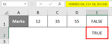
Look at the formula below; we have tested whether the cell A1 value is >20 or not, the B1 cell value is >20 or not, and the C1 cell value is >20.
In the above function, all the cell values are >20, so the result is “TRUE.” We will change one of the cell values to less than 20.

The B1 cell value changed to 18, less than 20, so the result is “FALSE,” even though the other two cell values are >20.
We will apply the OR function in excelThe OR function in Excel is used to test various conditions, allowing you to compare two values or statements in Excel. If at least one of the arguments or conditions evaluates to TRUE, it will return TRUE. Similarly, if all of the arguments or conditions are FALSE, it will return FASLE.read more for the same number.

For the OR function, one criterion needs to be satisfied to get the result as “TRUE.” So we need all the conditions to meet the “TRUE” result, unlike the AND function.
Example #2 – Multiple Logical Functions in Excel
Now, we will see how to perform multiple logical functions to match multiple conditions.
- Let us look at the below data in Excel.

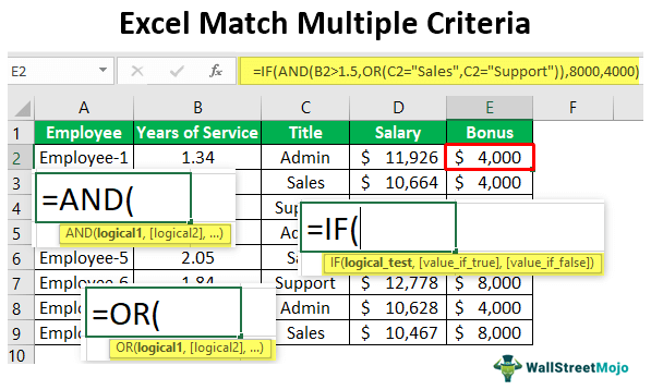
We need to calculate the “Bonus” amount based on the below conditions from the above data.
If the “Year of Service” is >1.5 years and if the “Department” is “Sales” or “Support,” then the bonus is $8,000; otherwise, the bonus will be $4,000.
So, to arrive at one result, we need to match multiple criteria in Excel. In this case, we need to test whether the “Year of Service” is 1.5 and whether the “Department” is “Sales” or “Support” to arrive at the bonus amount.
- We must first open the condition in Excel.

- The first logical condition to test is compulsory, whether the year of service is >1.5 years or not. So for the mandatory “TRUE” result, we need to use AND function.
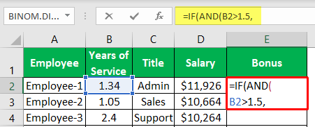
The above logical test will return “TRUE” only if the year of service is >1.5. Otherwise, we will get “FALSE” as a result. Inside this AND function, we need to test one more criterion, i.e., whether the “Department” is “Sales” or “Support,” to arrive at a bonus amount.
- If any department matches these criteria, we need the “TRUE” result, so we need to use the OR function.

As you can see above, we have used AND and OR functions to match single criteria. So, for example, the AND function will test the year of service at>1.5 years, and the OR function will test whether the department is “Sales” or “Support.” So if the “Year of Service” is 1.5 and the department is either “Sales” or “Support,” the logical test result will be “TRUE” or else “FALSE.”
- If the logical test is “TRUE,” we need the bonus amount at $8,000. So for the value, if True argument, we need to supply #8,000.

- If the logical test is “FALSE,” we need the bonus amount at $4,000.

- So, we are done with applying the formula, closing the formula, and applying the formula to other cells to get the result in other cells.

Now, let us look at the fourth row. In this case, the “Year of Service” is 2.4, and the “Department” is “Support,” so the bonus arrives at $8,000. Like this, we can match multiple criteria in Excel.
Things to Remember
- To test multiple criteria to arrive at a single result, we need to use multiple logical functions inside the IF condition.
- The AND and OR Excel functions are the two supporting functions we can use to test multiple criteria.
- The AND function in Excel may return “TRUE” only if all the logical tests are satisfied, but on the other hand, the OR function requires at least one logical test to be met to get a “TRUE” result.
Recommended Articles
This article has been a guide to Excel Match Multiple Criteria. Here, we discuss matching multiple criteria in Excel using AND, IF, and OR formulas and practical examples. You may learn more about Excel from the following articles: –
- Excel Break-Even Analysis
- Match Function Excel Examples
- VLOOKUP with Multiple Criteria
- SUMPRODUCT with Multiple Criteria
- NETWORKDAYS Excel Function
Excel Match Multiple Criteria (Table of Contents)
- Introduction to Match Multiple Criteria in Excel
- How to Match Multiple Criteria in Excel?
Introduction to Match Multiple Criteria in Excel
As a data analyst, you always need to deal with multiple criteria and conditions to get the desired result. In Excel, you can use the IF Statement for conditional outputs. However, at times you need to construct more sophisticated logical tests in order to get the desired results. It may include the multiple IF Statements (i.e. nested IF) or can also be achieved with the help of some logical operators used under IF statements. We ideally can construct multiple criteria’s using logical AND & OR operator under the IF Statement.
- AND Operator: If you use logical AND operator/keyword under IF Statement, you will get TRUE as a result if all conditions/criteria are satisfied. Otherwise, it will return FALSE.
- OR Operator: If you use logical OR operator/keyword under IF statement, you’ll get TRUE as a result if at least one of the multiple conditions/criteria are satisfied. Else it will return FALSE.
How to Match Multiple Criteria in Excel?
To Match Multiple Criteria in Excel is very simple and easy. Let’s understand this function with some examples.
You can download this Match Multiple Criteria Excel Template here – Match Multiple Criteria Excel Template
Example #1 – AND/OR Operators Works for Multiple Criteria
Suppose we have three sets of marks for a student as shown below:

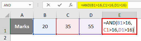
Step 1: In cell E1, as we need to check how AND operator works for multiple criteria, start initiating the formula by typing “=AND(
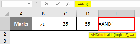
Step 2: We need to specify logical criteria under AND function. Use criteria as cell value greater than 16 for all cells (B1, C1, D1). You can use a comma as a separator to separate the multiple criteria conditions. See the screenshot below:
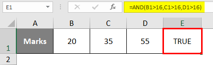
Once you press Enter key, you can see TRUE as a result in cell E1. Since all values present in cell B1, C1, and D1 are greater than 16, all the criteria are satisfied, leading to a Boolean output as TRUE under cell E1.
Step 3: Change the value in cell B1 as 12 and see how the result in cell E1 is affected.
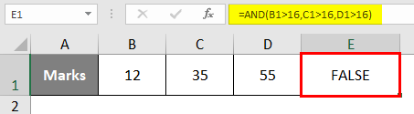
You can see with the same criteria under AND function, if we change the value under cell B1 as less than the criteria value (i.e. 16), we will get the output as FALSE. Since the value in cell B1 is not greater than 16, not all the criteria are satisfied.
Step 4: In cell E2, use the OR to check how it works; use the same criteria values. Ideally, OR gives Boolean output as TRUE if at least one of the criteria is satisfied.
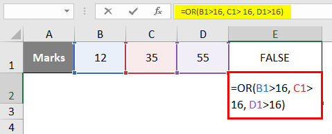
Press Enter key, and you can see the output as TRUE in cell E2 since C1 and D1 have values greater than 16. However, with E1, it is still FALSE since not all the conditions are satisfied.
Example #2 – Complex Criteria in Combination with IF, AND/OR
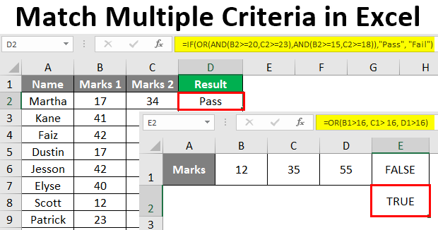
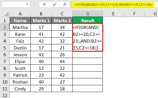
Suppose we conduct two tests in a class of 10 students and have Marks in both tests for each student stored under column Marks 1 and Marks 2 respectively. We wanted to check whether the student has passed the exam or not. See the screenshot of the below data.
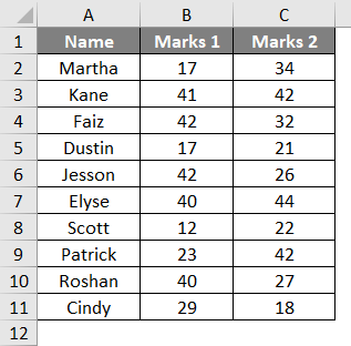
In order to check whether the student has passed the test or he failed, we can use a combination of IF statement with AND/OR operator to combine the multiple criteria.
Suppose we have two criteria’s under this example:
Criteria 1: Column B >= 20 and Column C >= 23
Criteria 2: Column B >= 15 and Column C >= 18
If either one of the criteria is fulfilled, the student will be declared as Pass; else, he/she will be declared as Fail. Let’s try to figure this tricky criterion out with IF, AND, OR.
Step 1: In cell D2, initiate the formula for IF Statement by typing “=IF(
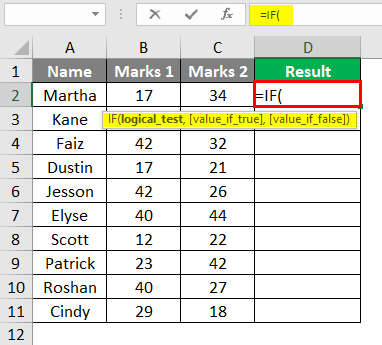
Step 2: Initiate an OR condition within the IF statement as shown below:
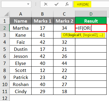
Step 3: Now, we need to add two AND conditions within this OR condition separated by a comma. Use (AND(B2>= 20, C2>=23), AND(B2>=15, C2>=18)) under OR condition within IF Statement and close the bracket for OR condition.
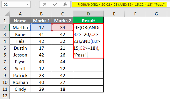
This condition will first check if Marks 1 and Marks 2 are greater than or equals to 20 and 23 respectively (first AND condition) OR if not, it will check whether the Marks 1 and Marks 2 are greater than or equals to 15 and 18 (second AND condition). If at least one of these two conditions is satisfied, the student will be considered as Pass; otherwise, the student will be considered a Fail.
Step 4: Add the [value_if_true] as “Pass” under the formula in cell D2 to specify if at least one of the condition gets satisfied, a student is a pass.
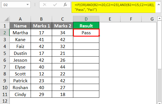
Step 5: Add “Fail” as a value for [value_if_false] under the IF statement to complete the formula and close the brackets to complete it. Press Enter key to see the output in cell D2 whether the student named “Martha” has passed the exam or not.
Step 6: Drag the formula across cells D2:D11 so that we will have a result value, either Pass or Fail, for all the students named in column A. You can select D2:D11 and then press Ctrl + D as a keyboard shortcut to be able to copy the formula across rows.
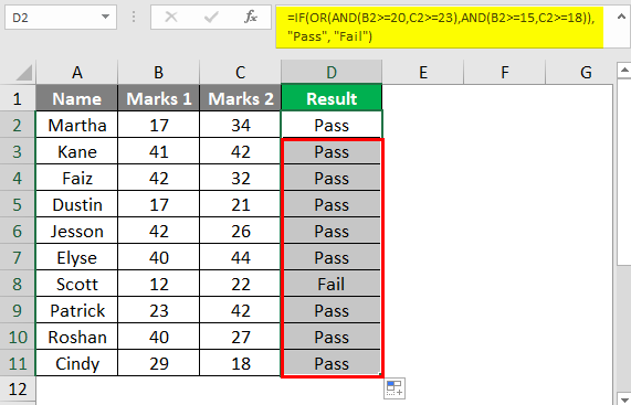
This is how we can match multiple criteria’s under Excel with the help of IF statement, AND & OR logical operators. This article ends here. Let’s wrap things up with some points to be remembered.
Things to Remember
- Logical operators such as AND, OR in combination with conditional statement IF are used to match multiple criteria under Excel.
- Microsoft Excel tests all the conditions under AND even if the previous condition is checked and appeared as FALSE. This is a bit unusual as in other programming languages if the previously checked condition is returned as FALSE under logical AND, the system stops checking other subsequent conditions.
- Logical AND returns TRUE if all the conditions inputted are satisfied. Otherwise, it returns as FALSE.
- Logical OR returns TRUE if at least one of the conditions is satisfied. If no other condition is satisfied, it returns as FALSE.
Recommended Article
This has been a guide to Excel Match Multiple Criteria. Here we discuss how to Match Multiple Criteria along with practical examples and a downloadable excel template. You can also go through our other suggested articles –
- INDEX MATCH Function in Excel
- Matching Columns in Excel
- VBA Match
- How to Match Data in Excel