Criteria for range excel - Word и Excel - помощь в работе с программами

If the data you want to filter requires complex criteria (such as Type = «Produce» OR Salesperson = «Davolio»), you can use the Advanced Filter dialog box.

To open the Advanced Filter dialog box, click Data > Advanced.

The Sort & Filter group on the Data tab

Advanced Filter	Example
Overview of advanced filter criteria
Multiple criteria, one column, any criteria true	Salesperson = «Davolio» OR Salesperson = «Buchanan»
Multiple criteria, multiple columns, all criteria true	Type = «Produce» AND Sales > 1000
Multiple criteria, multiple columns, any criteria true	Type = «Produce» OR Salesperson = «Buchanan»
Multiple sets of criteria, one column in all sets	(Sales > 6000 AND Sales < 6500 ) OR (Sales < 500)
Multiple sets of criteria, multiple columns in each set	(Salesperson = «Davolio» AND Sales >3000) OR (Salesperson = «Buchanan» AND Sales > 1500)
Wildcard criteria	Salesperson = a name with ‘u’ as the second letter

Overview of advanced filter criteria

The Advanced command works differently from the Filter command in several important ways.

It displays the Advanced Filter dialog box instead of the AutoFilter menu.
You type the advanced criteria in a separate criteria range on the worksheet and above the range of cells or table that you want to filter. Microsoft Office Excel uses the separate criteria range in the Advanced Filter dialog box as the source for the advanced criteria.

Sample data

The following sample data is used for all procedures in this article.

The data includes four blank rows above the list range that will be used as a criteria range (A1:C4) and a list range (A6:C10). The criteria range has column labels and includes at least one blank row between the criteria values and the list range.

To work with this data, select it in the following table, copy it, and then paste it in cell A1 of a new Excel worksheet.

Type	Salesperson	Sales




Type	Salesperson	Sales
Beverages	Suyama	$5122
Meat	Davolio	$450
produce	Buchanan	$6328
Produce	Davolio	$6544

Comparison operators

You can compare two values by using the following operators. When two values are compared by using these operators, the result is a logical value—either TRUE or FALSE.

Comparison operator	Meaning	Example
= (equal sign)	Equal to	A1=B1
> (greater than sign)	Greater than	A1>B1
< (less than sign)	Less than	A1<B1
>= (greater than or equal to sign)	Greater than or equal to	A1>=B1
<= (less than or equal to sign)	Less than or equal to	A1<=B1
<> (not equal to sign)	Not equal to	A1<>B1

Using the equal sign to type text or a value

Because the equal sign (=) is used to indicate a formula when you type text or a value in a cell, Excel evaluates what you type; however, this may cause unexpected filter results. To indicate an equality comparison operator for either text or a value, type the criteria as a string expression in the appropriate cell in the criteria range:

=»=
entry
»

Where entry is the text or value you want to find. For example:

What you type in the cell	What Excel evaluates and displays
=»=Davolio»	=Davolio
=»=3000″	=3000

Considering case-sensitivity

When filtering text data, Excel doesn’t distinguish between uppercase and lowercase characters. However, you can use a formula to perform a case-sensitive search. For an example, see the section Wildcard criteria.

Using pre-defined names

You can name a range Criteria, and the reference for the range will appear automatically in the Criteria range box. You can also define the name Database for the list range to be filtered and define the name Extract for the area where you want to paste the rows, and these ranges will appear automatically in the List range and Copy to boxes, respectively.

Creating criteria by using a formula

You can use a calculated value that is the result of a formula as your criterion. Remember the following important points:

The formula must evaluate to TRUE or FALSE.
Because you are using a formula, enter the formula as you normally would, and do not type the expression in the following way:

=»=
entry
»
Do not use a column label for criteria labels; either keep the criteria labels blank or use a label that is not a column label in the list range (in the examples that follow, Calculated Average and Exact Match).

If you use a column label in the formula instead of a relative cell reference or a range name, Excel displays an error value such as #NAME? or #VALUE! in the cell that contains the criterion. You can ignore this error because it does not affect how the list range is filtered.
The formula that you use for criteria must use a relative reference to refer to the corresponding cell in the first row of data.
All other references in the formula must be absolute references.

Multiple criteria, one column, any criteria true

Boolean logic: (Salesperson = «Davolio» OR Salesperson = «Buchanan»)

Insert at least three blank rows above the list range that can be used as a criteria range. The criteria range must have column labels. Make sure that there is at least one blank row between the criteria values and the list range.

To find rows that meet multiple criteria for one column, type the criteria directly below each other in separate rows of the criteria range. Using the example, enter:

Type	Salesperson	Sales
	=»=Davolio»
	=»=Buchanan»

Click a cell in the list range. Using the example, click any cell in the range A6:C10.
On the Data tab, in the Sort & Filter group, click Advanced.
Do one of the following:
- To filter the list range by hiding rows that don’t match your criteria, click Filter the list, in-place.
- To filter the list range by copying rows that match your criteria to another area of the worksheet, click Copy to another location, click in the Copy to box, and then click the upper-left corner of the area where you want to paste the rows.
  
  Tip When you copy filtered rows to another location, you can specify which columns to include in the copy operation. Before filtering, copy the column labels for the columns that you want to the first row of the area where you plan to paste the filtered rows. When you filter, enter a reference to the copied column labels in the Copy to box. The copied rows will then include only the columns for which you copied the labels.
In the Criteria range box, enter the reference for the criteria range, including the criteria labels. Using the example, enter $A$1:$C$3.

To move the Advanced Filter dialog box out of the way temporarily while you select the criteria range, click Collapse Dialog .

Using the example, the filtered result for the list range is:

Type	Salesperson	Sales
Meat	Davolio	$450
produce	Buchanan	$6,328
Produce	Davolio	$6,544

Multiple criteria, multiple columns, all criteria true

Boolean logic: (Type = «Produce» AND Sales > 1000)

Insert at least three blank rows above the list range that can be used as a criteria range. The criteria range must have column labels. Make sure that there is at least one blank row between the criteria values and the list range.

To find rows that meet multiple criteria in multiple columns, type all the criteria in the same row of the criteria range. Using the example, enter:

Type	Salesperson	Sales
=»=Produce»		>1000

Click a cell in the list range. Using the example, click any cell in the range A6:C10.
On the Data tab, in the Sort & Filter group, click Advanced.
Do one of the following:
- To filter the list range by hiding rows that don’t match your criteria, click Filter the list, in-place.
- To filter the list range by copying rows that match your criteria to another area of the worksheet, click Copy to another location, click in the Copy to box, and then click the upper-left corner of the area where you want to paste the rows.
  
  Tip When you copy filtered rows to another location, you can specify which columns to include in the copy operation. Before filtering, copy the column labels for the columns that you want to the first row of the area where you plan to paste the filtered rows. When you filter, enter a reference to the copied column labels in the Copy to box. The copied rows will then include only the columns for which you copied the labels.
In the Criteria range box, enter the reference for the criteria range, including the criteria labels. Using the example, enter $A$1:$C$2.

To move the Advanced Filter dialog box out of the way temporarily while you select the criteria range, click Collapse Dialog .

Using the example, the filtered result for the list range is:

Type	Salesperson	Sales
produce	Buchanan	$6,328
Produce	Davolio	$6,544

Multiple criteria, multiple columns, any criteria true

Boolean logic: (Type = «Produce» OR Salesperson = «Buchanan»)

Insert at least three blank rows above the list range that can be used as a criteria range. The criteria range must have column labels. Make sure that there is at least one blank row between the criteria values and the list range.

To find rows that meet multiple criteria in multiple columns where any criteria can be true, type the criteria in the different columns and rows of the criteria range. Using the example, enter:

Type	Salesperson	Sales
=»=Produce»
	=»=Buchanan»

Click a cell in the list range. Using the example, click any cell in the list range A6:C10.
On the Data tab, in the Sort & Filter group, click Advanced.
Do one of the following:
- To filter the list range by hiding rows that don’t match your criteria, click Filter the list, in-place.
- To filter the list range by copying rows that match your criteria to another area of the worksheet, click Copy to another location, click in the Copy to box, and then click the upper-left corner of the area where you want to paste the rows.
Tip: When you copy filtered rows to another location, you can specify which columns to include in the copy operation. Before filtering, copy the column labels for the columns that you want to the first row of the area where you plan to paste the filtered rows. When you filter, enter a reference to the copied column labels in the Copy to box. The copied rows will then include only the columns for which you copied the labels.
In the Criteria range box, enter the reference for the criteria range, including the criteria labels. Using the example, enter $A$1:$B$3.

To move the Advanced Filter dialog box out of the way temporarily while you select the criteria range, click Collapse Dialog .

Using the example, the filtered result for the list range is:

Type	Salesperson	Sales
produce	Buchanan	$6,328
Produce	Davolio	$6,544

Multiple sets of criteria, one column in all sets

Boolean logic: ( (Sales > 6000 AND Sales < 6500 ) OR (Sales < 500) )

Insert at least three blank rows above the list range that can be used as a criteria range. The criteria range must have column labels. Make sure that there is at least one blank row between the criteria values and the list range.

To find rows that meet multiple sets of criteria where each set includes criteria for one column, include multiple columns with the same column heading. Using the example, enter:

Type	Salesperson	Sales	Sales
		>6000	<6500
		<500

Click a cell in the list range. Using the example, click any cell in the list range A6:C10.
On the Data tab, in the Sort & Filter group, click Advanced.
Do one of the following:
- To filter the list range by hiding rows that don’t match your criteria, click Filter the list, in-place.
- To filter the list range by copying rows that match your criteria to another area of the worksheet, click Copy to another location, click in the Copy to box, and then click the upper-left corner of the area where you want to paste the rows.
  
  Tip: When you copy filtered rows to another location, you can specify which columns to include in the copy operation. Before filtering, copy the column labels for the columns that you want to the first row of the area where you plan to paste the filtered rows. When you filter, enter a reference to the copied column labels in the Copy to box. The copied rows will then include only the columns for which you copied the labels.
In the Criteria range box, enter the reference for the criteria range, including the criteria labels. Using the example, enter $A$1:$D$3.

To move the Advanced Filter dialog box out of the way temporarily while you select the criteria range, click Collapse Dialog .

Using the example, the filtered result for the list range is:

Type	Salesperson	Sales
Meat	Davolio	$450
produce	Buchanan	$6,328

Multiple sets of criteria, multiple columns in each set

Boolean logic: ( (Salesperson = «Davolio» AND Sales >3000) OR (Salesperson = «Buchanan» AND Sales > 1500) )

Insert at least three blank rows above the list range that can be used as a criteria range. The criteria range must have column labels. Make sure that there is at least one blank row between the criteria values and the list range.

To find rows that meet multiple sets of criteria, where each set includes criteria for multiple columns, type each set of criteria in separate columns and rows. Using the example, enter:

Type	Salesperson	Sales
	=»=Davolio»	>3000
	=»=Buchanan»	>1500

Click a cell in the list range. Using the example, click any cell in the list range A6:C10.
On the Data tab, in the Sort & Filter group, click Advanced.
Do one of the following:
- To filter the list range by hiding rows that don’t match your criteria, click Filter the list, in-place.
- To filter the list range by copying rows that match your criteria to another area of the worksheet, click Copy to another location, click in the Copy to box, and then click the upper-left corner of the area where you want to paste the rows.
  
  Tip When you copy filtered rows to another location, you can specify which columns to include in the copy operation. Before filtering, copy the column labels for the columns that you want to the first row of the area where you plan to paste the filtered rows. When you filter, enter a reference to the copied column labels in the Copy to box. The copied rows will then include only the columns for which you copied the labels.
In the Criteria range box, enter the reference for the criteria range, including the criteria labels. Using the example, enter $A$1:$C$3.To move the Advanced Filter dialog box out of the way temporarily while you select the criteria range, click Collapse Dialog .

Using the example, the filtered result for the list range would be:

Type	Salesperson	Sales
produce	Buchanan	$6,328
Produce	Davolio	$6,544

Wildcard criteria

Boolean logic: Salesperson = a name with ‘u’ as the second letter

To find text values that share some characters but not others, do one or more of the following:

Type one or more characters without an equal sign (=) to find rows with a text value in a column that begin with those characters. For example, if you type the text Dav as a criterion, Excel finds «Davolio,» «David,» and «Davis.»

Use a wildcard character.

Use	To find
? (question mark)	Any single character For example, sm?th finds «smith» and «smyth»
* (asterisk)	Any number of characters For example, *east finds «Northeast» and «Southeast»
~ (tilde) followed by ?, *, or ~	A question mark, asterisk, or tilde For example, fy91~? finds «fy91?»

Insert at least three blank rows above the list range that can be used as a criteria range. The criteria range must have column labels. Make sure that there is at least one blank row between the criteria values and the list range.

In the rows below the column labels, type the criteria that you want to match. Using the example, enter:

Type	Salesperson	Sales
=»=Me*»
	=»=?u*»

Click a cell in the list range. Using the example, click any cell in the list range A6:C10.
On the Data tab, in the Sort & Filter group, click Advanced.
Do one of the following:
- To filter the list range by hiding rows that don’t match your criteria, click Filter the list, in-place
- To filter the list range by copying rows that match your criteria to another area of the worksheet, click Copy to another location, click in the Copy to box, and then click the upper-left corner of the area where you want to paste the rows.
  
  Tip: When you copy filtered rows to another location, you can specify which columns to include in the copy operation. Before filtering, copy the column labels for the columns that you want to the first row of the area where you plan to paste the filtered rows. When you filter, enter a reference to the copied column labels in the Copy to box. The copied rows will then include only the columns for which you copied the labels.
In the Criteria range box, enter the reference for the criteria range, including the criteria labels. Using the example, enter $A$1:$B$3.

To move the Advanced Filter dialog box out of the way temporarily while you select the criteria range, click Collapse Dialog .

Using the example, the filtered result for the list range is:

Type	Salesperson	Sales
Beverages	Suyama	$5,122
Meat	Davolio	$450
produce	Buchanan	$6,328

Need more help?

You can always ask an expert in the Excel Tech Community or get support in the Answers community.

Источник

One of the most important skills of building useful formulas is creating criteria – the part of a formula that decides what to include or exclude in a calculation. However, it can be surprisingly tricky to build effective criteria because it requires a good understanding of how Excel handles data. If you’ve ever spent an afternoon troubleshooting a formula that seems like it should «just work», you know what I mean

This guide aims to help you build formulas that work the first time.

Note: language mavens will point out that «criterion» is singular and «criteria» is plural, but I’m going to use «criteria» in both cases to keep things simple.

Function names on dark backgrounds below are links to more information.

What do criteria do?

Among other things, criteria:

Direct logical flow with IF/THEN logic
Restrict processing to matching values only
Create conditional sums and counts
Filter data to exclude irrelevant information
Trigger conditional formatting rules

To help set the stage, let’s look at three examples of criteria in action.

Example #1

In the screen below, F3 contains this formula:

=IF(E3>30,"Yes","No")

Translation: If the value in E3 is greater than 30, return «Yes», otherwise return «No».

Here, E3>30 is the criteria, used inside IF to determine if the formula should return «Yes» or «No» for each invoice.

Example #2

In the next example, D3 contains this formula:

=IF(OR(B3="red",B3="green"),C3*1.1,C3)

Translation: if B3 is either «red» or «green», increase the price by 10%. Otherwise, return the original price.

Example #3

In this example, the SUMIFS function is used to sum the total only when the color is «red»:

=SUMIFS(E3:E7,B3:B7,"red")

Translation: sum values in E3:E7 when value in B3:B7 is «red».

Criteria Basics

This section covers the building blocks of formula criteria, and some simple ways to verify that criteria are performing as expected.

What are criteria?

Criteria are logical expressions that return TRUE or FALSE, or their numerical equivalents, 1 or 0.

That’s it.

The trick is to construct criteria in a way so that they only return TRUE when the test meets your exact criteria. In all other cases, criteria should return FALSE or zero. If you can master this one idea, you have the foundation to build and understand many advanced formulas.

Logical operators

Criteria often make use of the logical operators listed in the table below.

Operator	Meaning	Example
=	Equal to	=A1=10
<>	Not equal to	=A1<>10
>	Greater than	=A1>100
<	Less than	=A1<100
>=	Greater than or equal to	=A1>=75
<=	Less than or equal to	=A1<=0

Logical operators can be combined in various ways, as seen in the examples below.

Logical functions

Excel has several so-called «logical functions» that can be used to construct and utilize conditions. The table below lists the key logical functions.

Function	Purpose
IF	Test one condition; direct logical flow
IFS	Test multiple conditions; direct logical flow
NOT	Reverse criteria or results
AND	Test multiple conditions, return TRUE if all are TRUE
OR	Test multiple conditions, return TRUE if at least one is TRUE
XOR	Exclusive OR – return TRUE if one or the other, not both
IFERROR	Trap errors and return alternative results

Multiple criteria

Naturally, there are many cases where you will want to use multiple criteria. In simple situations, you can use the AND, OR, and NOT functions. Here are a few examples:

=AND(A1>0,A1<10) // greater than 0 and less than 10
=OR(A1="red",A1="blue") // red or blue
=NOT(OR(A1="red",A1="blue")) // not red or blue
=AND(ISNUMBER(A1),A1>100) // number greater than 100

Wildcards

Excel provides three «wildcards» for matching text in formulas:

Character	Name	Purpose
*	Asterisk	Match zero or more characters
?	Question mark	Match any one character
~	Tilde	Match literal wildcard

Wildcards can be used alone or combined to get a variety of matching behaviors:

Usage	Behavior	Will match
?	Any one character	«A», «B», «c», «z», etc.
??	Any two characters	«AA», «AZ», «zz», etc.
???	Any three characters	«Jet», «AAA», «ccc», etc.
*	Any characters	«apple», «APPLE», «A100», etc.
*th	Ends in «th»	«bath», «fourth», etc.
c*	Starts with «c»	«Cat», «CAB», «cindy», «candy», etc.
?*	At least one character	«a», «b», «ab», «ABCD», etc.
???-??	5 characters with hypen	«ABC-99″,»100-ZT», etc.
*~?	Ends in question mark	«Hello?», «Anybody home?», etc.
xyz	Contains «xyz»	«code is XYZ», «100-XYZ», «XyZ90», etc.

Here are a few examples of using wildcards for criteria in the COUNTIFS function.

=COUNTIFS(A1:A100,"*red*") // count cells that contain "red"
=COUNTIFS(A1:A100, "www*") // count cells starting with "www"
=COUNTIFS(A1:A100,"?????") // count cells with 5 characters

Not all functions allow wildcards. Here is a list of common functions that do:

AVERAGEIF, AVERAGEIFS
COUNTIF, COUNTIFS
SUMIF, SUMIFS
VLOOKUP, HLOOKUP
MATCH
SEARCH

Notice the IF function is not on this list. To get wildcard behavior with IF, you can combine the SEARCH and ISNUMBER functions, as described below.

Testing criteria

The classic way to test criteria is to wrap them in the IF function. For example, to check for «red» or «blue», we can wrap the OR function inside IF like this:

=IF(OR(B3="red",B3="blue"),"OK", "")

Translation: if color is «red» or «blue», return «OK». Otherwise return nothing.

However, you can also test criteria directly on the worksheet as a formula. Let’s say you want to process values that are 80 and higher. In the screen below, C3 contains this formula, copied down.

=B3>=80

Translation: the value in B3 is greater than or equal to 80.

Without IF or another function, we only get a result of TRUE or FALSE, but it’s enough to verify criteria are working as expected.

Don’t be thrown off by the equals (=) sign when testing criteria as a formula. All Excel formulas must begin with an equals sign, so it must be included. Remove the equal sign when you move criteria into another formula.

Another way to test criteria is to use F9 to evaluate criteria in place. Just carefully select a logical expression, and press F9. Excel will immediately evaluate the expression and display the result.

Video: How to use F9 to debug a formula.

Adding criteria to formulas

Of course, in most cases, you don’t want to return TRUE or FALSE to a cell, you want to return some other value based on criteria returning TRUE or FALSE. To do that, just remove the equal sign and add the criteria where needed in the formula.

In the example below, the formula C3 contains this formula, which uses the criteria above as the logical test inside IF:

=IF(B3>=80,"Pass","Fail")

Translation: if the value in B3 is greater than or equal to 80, return «Pass». Otherwise, return «Fail».

Criteria Examples

This section shows examples of how to build criteria to accomplish a variety of tasks for different kinds of content.

Blank or not blank

There are several ways you can check for blank or non-blank cells. To return TRUE if A1 is blank, you can use either:

=ISBLANK(A1)
=A1=""

To reverse the logic and check for non-blank cells, you can use:

=NOT(ISBLANK(A1))
=A1<>""

Another way to test for a blank cell is to check count characters:

=LEN(A1)=0

If the count is zero, the cell is «blank». This formula is useful when testing cells that may contain formulas that return empty strings («»). ISBLANK(A1) will return FALSE if a formula returns an empty string in A1, but LEN(A1)=0 will return TRUE.

Criteria for text

To return TRUE if a cell contains «red», you can use:

=A1="red"

To reverse logic, you can use the NOT function or the not equals to operator (<>) like this:

=NOT(A1="red")
=A1<>"red"

Notice in each case the text IS enclosed in double quotes (e.g. «red»). If you don’t use quotes, Excel will think you are trying to reference a named range or a function, and will return the #NAME error.

Criteria for numbers

To test if A1 is equal to 5, you can use criteria like this:

=A1=5 // TRUE if A1 equals 5

Here are some other examples of criteria to test numeric values:

=A1<100 // less than 100
=A1>=1 // greater than or equal to 1
=A1<>0 // not equal to zero
=AND(A1>0,A1<5) // greater than zero, less than 5
=MOD(A1,3)=0 // value is a multiple of 3

Notice numbers are NOT enclosed in double quotes. If you enclose a number in quotes, you are telling Excel to treat the number as text, which will make the criteria useless. Also, remember that number formatting in Excel affects display only, and does not change numeric data in any way. Do not include dollar signs ($), percent signs (%), or other formatting information when building criteria to test numbers.

Criteria for dates

Dates in Excel are just numbers, which means you are free to use ordinary math operations on dates if you like. With Order dates in column A and Delivery dates in column B, this formula in column C will mark delivery times greater than 3 days as «late»:

=IF((B2-A2)>3,"Late","")

Excel also provides a large number of specific functions for working with dates. For example, to check if a date is «in the future» you can use the TODAY function like this:

=A1>TODAY()

To check if a date occurs in the next 30 days, the formula can be extended to:

=AND(A1>TODAY(),A1<=(TODAY()+30))

Translation: IF A2 is greater than today AND less than or equal today + 30 days, return TRUE.

Here are a few other examples of criteria for dates, assuming A1 contains a valid date:

=DAY(A1)>15 // greater than 15th
=MONTH(A1)=6 // month is June
=YEAR(A1) = 2019 // year is 2019
=WEEKDAY(A1)=2 // date is a Monday

The safest way to insert a valid date into criteria is to use the DATE function, which accepts year, month, and day as separate arguments. Here are a couple examples:

=A1>DATE(2019,1,1) // after Jan. 1, 2019
=AND(A1>=DATE(2018,6,1),B4<=DATE(2018,8,31)) // Jun-Aug 2018

Criteria for times

Times are fractional numbers in Excel, so you can use simple math for time in some cases. For example, to check if a time in A1 is after 12:00 PM (more than 12 hours), you can use:

=A1>.5

This works because 1 day = 24 hours, so a half day = 12 hours.

For more granular work, Excel has special functions to extract time by component. For example, with the time 8:45 AM in cell A1:

=HOUR(A1) // returns 8
=MINUTE(A1) // returns 45
=SECOND(A1) // returns 0

The safest way to insert a time in criteria is to use the TIME function. Here are some examples:

=A1>TIME(9,15,0) // after 9:15 AM
=AND(A1>=TIME(9,0,0),A1<=TIME(17,0,0)) // 9 AM to 5 PM

Criteria for SUMIFS, COUNTIFS, etc.

The criteria for SUMIFS, COUNTIFS, AVERAGEIFS, and similar range-based functions follow slightly different rules. This is because the criteria are split into two parts (criteria range and criteria), and this impacts the syntax when criteria include operators.

Simple criteria based on equality don’t need special handling. The equals (=) operator is implied, so there’s no need to include it in criteria:

=COUNTIFS(A1:A100,10) // count cells equal to 10
=COUNTIFS(A1:A100,"red") // count cells that equal "red"

However, things change when we add operators:

=COUNTIFS(A1:A100,">10") // count cells greater than 10
=COUNTIFS(A1:A100,"<0") // count cells less than zero

Notice the quotes («») around the criteria? These are required when criteria include an operator in these functions.

Criteria for data types

Excel allows three main data types: text, numbers, and logicals. Dates, times, percentages, and fractions are all just numbers with number formatting applied to change the way they are displayed. By default, numbers are right-aligned, text is left-aligned, and logical values are centered. But a user can override alignment manually, so this is not a good test of type.

Excel provides three functions you can use to check data types: ISTEXT, ISNUMBER, and ISLOGICAL. These functions return TRUE or FALSE. In the screen below, the cells D3, F3, and H3 contain these formulas, copied down:

=ISTEXT(B3)
=ISNUMBER(B3)
=ISLOGICAL(B3)

To use these functions as criteria, just place them in the correct location of a formula. For example, to check if A1 contains a number, you can use ISNUMBER as the logical test inside IF like this:

=IF(ISNUMBER(B3),"OK","Invalid")

Note: Formulas are not a data type, but you can check for formulas with the ISFORMULA function:

=ISFORMULA(A1) // TRUE if A1 contains formula

Getting fancy

The examples above show the fundamentals of using criteria in formulas, there are many ways to make criteria more sophisticated. This section explores a few techniques.

Making criteria variable

It is often useful to make criteria variable, by referencing a cell on the worksheet. For example, in the worksheet below, the passing score is in cell E3, and the formula to determine pass or fail looks like this:

=IF(B3>=$E$3,"Pass","Fail")

Placing the passing score in cell E3 makes it easy to change at any time without editing formulas. Note that the reference to $E$3 is absolute to prevent changes as the formula is copied down.

Making criteria variable in COUNTIFS, SUMIFS, etc.

As before, if criteria are testing for equality, no special handling is needed:

=COUNTIF(range,A1) // count cells equal to A1

However, if criteria include operators, you’ll need to use concatenation. For example, to count cells greater than A1, you ‘ll need to join «>» to «A1» like this:

=COUNTIF(range,">"&A1)

The concatenation runs first. If A1 contains the number 10, this is the formula after concatenation:

=COUNTIF(range,">10")

Notice the pattern is the same as explained earlier – if criteria includes operators, it must appear in quotes («»).

Here are more examples of using concatenation in criteria:

=COUNTIF(range,"<"&B1) // count less than value in B1
=COUNTIF(range,"<>"&"") // count not blank cells
=COUNTIF(range,"*"&B1&"*") // count contains text in B1
=COUNTIF(range,">"&TODAY()) // count dates in future
=COUNTIF(range,"<"&TODAY()+7) // count up to 7 days from today

Contains specific text

One tricky situation is when you want to test if a cell contains specific text. For functions that support wildcards (like COUNTIFS, SUMIFS, etc.), you can use wildcards to do this. For example, to count cells that contain «red» anywhere in a cell with COUNTIFS, you can use an asterisk like this:

=COUNTIFS(A1:A100,"*red*")

However, many other functions (like the IF function) don’t support wildcards. In that case, you can combine ISNUMBER and SEARCH to create criteria that checks a cell for a partial match. In the screen below, D3 contains this formula:

=ISNUMBER(SEARCH(C3,B3))

You can use this expression as criteria inside IF like this

=IF(ISNUMBER(SEARCH("red",A1)),"red", "")

Translation: if «red» is found anywhere in A1, return «red».

This works because SEARCH returns a numeric position if «red» is found, and ISNUMBER returns TRUE. If not, SEARCH returns an error, and ISNUMBER returns FALSE. For more details, see this page.

Nested IFs

Nested IF formulas are often used to check multiple criteria and return multiple results. In general, the challenge is to build nested IFs so that the critieria run in the right sequence. For example, here is a nested IF formula that assigns a letter grade based on a numeric score:

=IF(C5<64,"F",IF(C5<73,"D",IF(C5<85,"C",IF(C5<95,"B","A"))))

Notice we are testing for low scores first, then progressively higher scores.

More: 19 tips for nested IFs (with alternatives)

Array constants in criteria

Array constants are hard-coded arrays with fixed values like this: {«A»,»B»,»C»}. They can sometimes be used as criteria to create simple OR logic criteria. For example, in the screen below, cell F4 contains this formula:

=SUM(SUMIFS(C3:C7,B3:B7,{"red","gold"}))

Translation: SUM sales where the color is «red» OR «gold».

Because we give SUMIFS two values for criteria, it returns two results. The SUM function then returns the sum of the two results.

Simple array formula criteria

Array formulas are a complicated topic, but the criteria for simple array formulas can be quite simple. A classic example is using the IF function to «filter out» values that should be excluded, then processing the result with another function.

In the screen below, the formula in G4 is:

{=MAX(IF(regions=F4,totals))}

where regions is the named range B3:B8 and totals is the named range D3:D8.

Note: this is an array formula and must be entered with control + shift + enter.

The result is the top value for each region.

For criteria, we use the expression:

regions=F4

This compares all region values with «West» from F4, and returns the following array result in the logical test for IF:

{TRUE;FALSE;TRUE;FALSE;TRUE;FALSE}

The final array returned by IF looks like this:

{10500;FALSE;12500;FALSE;11800;FALSE}

Only values associated with the «West» region make it into the array. Values associated with the «East» region are FALSE.

The MAX function then returns the largest value in the array, ignoring all FALSE values.

Advanced formula criteria

Below are links to more advanced formula criteria examples. Each link has a screenshot and a full explanation.

Count cells that contain errors
Sum if value is equal to one of many
COUNTIFS with multiple criteria and OR logic
Get nth largest value with criteria
Sum top n values with criteria
INDEX and MATCH with multiple criteria

More formula resources

The following links contain more detailed information on Excel formulas:

How to build logical formulas (video)
19 tips for nested IF formulas
30+ conditional formatting formulas
Core Formula (paid training)

Источник

And Criteria

Enter the criteria shown below on the worksheet.
Click any single cell inside the data set.
On the Data tab, in the Sort & Filter group, click Advanced.
Click in the Criteria range box and select the range A1:D2 (blue).
Click OK.

Contents

1 What is criteria range in Excel?
2 What is criteria range?
3 What is list range and criteria range in Excel?
4 How do I fix criteria in Excel?
5 What are examples of criteria?
6 How do you filter ranges in Excel?
7 How do I create a filter box in Excel?
8 What are 5 examples of criteria?
9 How do you make a criteria?
10 What are 5 types of criteria?
11 What is criteria range in advanced filter?
12 How do you convert a table to a range in Excel?
13 How do I create a data validation list in Excel based on criteria?
14 How do I extract a list from criteria in Excel?
15 How do you define a range based on another cell value in Excel?
16 How do I create a dynamic filter in Excel?
17 How do I create a simple search box in Excel?
18 What are the 3 criteria?
19 How do you use criteria correctly?
20 What is a criteria list?

The criteria argument is a worksheet range that contains the criteria—it is not the actual criteria. At the simplest, for a single criterion, this is a two-cell range that is one column wide and two rows high.

What is criteria range?

Criteria-range meaning
Conditions for selecting records; for example, “Illinois customers with balances over $10,000” or “residents who have lived in the state less than five years.”

What is list range and criteria range in Excel?

The data includes four blank rows above the list range that will be used as a criteria range (A1:C4) and a list range (A6:C10). The criteria range has column labels and includes at least one blank row between the criteria values and the list range.

How do I fix criteria in Excel?

All Excel formulas must begin with an equals sign, so it must be included. Remove the equal sign when you move criteria into another formula. Another way to test criteria is to use F9 to evaluate criteria in place. Just carefully select a logical expression, and press F9.

What are examples of criteria?

Criteria is defined as the plural form of criterion, the standard by which something is judged or assessed. An example of criteria are the various SAT scores which evaluate a student’s potential for a successful educational experience at college. Plural form of criterion. (nonstandard, proscribed) A single criterion.

How do you filter ranges in Excel?

Filter a range of data

Select any cell within the range.
Select Data > Filter.
Select the column header arrow .
Select Text Filters or Number Filters, and then select a comparison, like Between.
Enter the filter criteria and select OK.

How do I create a filter box in Excel?

To filter with search:

Select the Data tab, then click the Filter command. A drop-down arrow will appear in the header cell for each column.
Click the drop-down arrow for the column you want to filter.
The Filter menu will appear.
When you’re done, click OK.
The worksheet will be filtered according to your search term.

What are 5 examples of criteria?

20 Examples of Decision Criteria

Cost. A budget, cost constraint or preference for lower cost options.
Opportunity Costs.
Return on Investment.
Time.
Quality.
Customer Experience.
Performance.
Reliability.

How do you make a criteria?

How to write key selection criteria

Step 1: brainstorm key words and ideas. Copy and paste the criteria from the position description into a new document.
Step 2: write a statement using the SAO approach. Write a statement under each criterion of 60 to 120 words using the SAO approach:
Step 3: proofread your statements.

What are 5 types of criteria?

The following are illustrative examples.

Scores. A minimum score on a standard test that is required to be considered for admissions into a university or college.
Scoring Structure. A structure for scoring.
Principles.
Rules.
Guidelines.
Requirements.
Specifications.
Algorithms.

What is criteria range in advanced filter?

In the criteria range for an Excel advanced filter, you can set the rules for the data that should remain visible after the filter is applied. You can use one criterion, or several.

How do you convert a table to a range in Excel?

Convert an Excel table to a range of data

Click anywhere in the table and then go to Table Tools > Design on the Ribbon.
In the Tools group, click Convert to Range. -OR- Right-click the table, then in the shortcut menu, click Table > Convert to Range.

How do I create a data validation list in Excel based on criteria?

To perform this, select a range of cells and under the Data tab select the Data Validation option. In the Data Validation Dialogue box, select the Custom option as Validation Criteria. In the formula section, write =$B$2=”Insert Data” and press OK. Now in the selected range put any data you want and press enter.


How do I extract a list from criteria in Excel?
5. Extract all rows from a range that meet criteria in one column [Excel defined Table]

Select a cell in the dataset.
Press CTRL + T.
Press with left mouse button on check box "My table has headers".
Press with left mouse button on OK button.

How do you define a range based on another cell value in Excel?
Define range based on cell value
 To do calculation for a range based on another cell value, you can use a simple formula. Select a blank cell which you will put out the result, enter this formula =AVERAGE(A1:INDIRECT(CONCATENATE("A",B2))), and press Enter key to get the result.
How do I create a dynamic filter in Excel?
Step 2 – Creating The Dynamic Excel Filter Search Box

Go to Developer Tab –> Controls –> Insert –> ActiveX Controls –> Combo Box (ActiveX Controls).
Click anywhere on the worksheet.
Right-click on Combo Box and select Properties.
In Properties window, make the following changes:

How do I create a simple search box in Excel?
To create a search box in Excel, go to Conditional Formatting, which is under the Home menu ribbon, and from the drop-down menu, the list creates a new rule to use a formula for formatting a cell from there.
What are the 3 criteria?
THREE CRITERIA: KNOWLEDGE, CONVICTION, AND SIGNIFICANCE.
How do you use criteria correctly?
Criterion is just the singular form. In other words, “criterion” refers to a single thing, while “criteria” refers to two or more things. That's it! To say it another way, the only criterion for proper use of the word “criteria” is that you are listing several items.
What is a criteria list?
The criteria list can be used as a tool to discuss the potential of ideas. Participants can use it to explain why they like a certain idea. The problem owner decides, but even a problem owner needs advisers who point out the pros and cons of different approaches.

Источник

A lesson on how to filter based on a list in Excel by SpreadsheetClass.com

When filtering data in Excel you may sometimes need to filter by an entire list of values, rather than by just a single/few specified values. There is a way to do this by using formulas, and it is fairly easy! You can use the FILTER and COUNTIF functions to filter based on a list in Excel.

To filter by a list in Excel, use the COUNTIF function to give an indication of whether or not each row meets your criteria, and then use the FILTER function to filter out the rows that do not meet your criteria.

There is also a way to filter by a list without using formulas, but it takes longer and is more difficult. Simply using formulas is the easiest way to filter by a list in Excel.

To filter by a list of values in Excel, do the following:

Use the COUNTIF function to check whether or not each row in your source data should be included in your filter results (i.e. Check to see if any of the values in the list to filter by are found within your data to be filtered). Example: =COUNTIF(F2:F10,A3)
Use the FILTER function to filter the source data, using the column that the COUNTIF function is in as the criteria column. Example: =FILTER(A3:C100,D3:D100=1)

Here are formulas that you can use to filter by a list in Excel:

The COUNTIF and FILTER formulas below must both be used to accomplish the task of filtering by a list of items / criteria. Further below I will teach you how to use these formulas together in your sheet to file by a list.

Filter Where Found in List

=COUNTIF(F2:F12,A3)

=FILTER(A3:C17,D3:D17=1)

FILTER Where NOT in List

=COUNTIF(F2:F12,A3)

=FILTER(A3:C17,D3:D17<>1)

Filter by list from another sheet

=COUNTIF(‘Tab 2’!A2:A12,A3)

=FILTER(A3:C17,D3:D17=1)

Alternate: =FILTER(‘Tab 1′!A3:C17,’Tab 1’!D3:D17=1)

In this article I will stick to using the FILTER and COUNTIF functions, since this is the faster and more reliable choice for filtering a range by an array in Excel.

This article focuses on filtering by a list in Excel, but check out this article if you want to learn how to filter by a list in Google Sheets.

If you want to learn how to use the FILTER function to perform ordinary filtering tasks, here is an article that will help you learn the FILTER function from the ground up.

But here we will only be filtering by lists/arrays/columns of data.

I have provided multiple examples showing the different ways to set up the formulas depending on how your data is arranged (i.e. depending on which tab your data/formula is on).

Filter rows based on a list in one sheet vs. multiple sheets

To start with, we will put our formula, our unfiltered data, and the list to filter by, all on the same tab so that you can easily see how the formula is set up and how it functions. But further below I will show you how to use multiple tabs while filtering by a list.

In the first examples we will start very simple, and filter a range of data, by a single-column / list, where the list that we are going to filter by does not contain any extra entries that are not present in the source data (data to be filtered).

This is not always how it will be in the real world… but this will make it easy to see what the formula is doing.

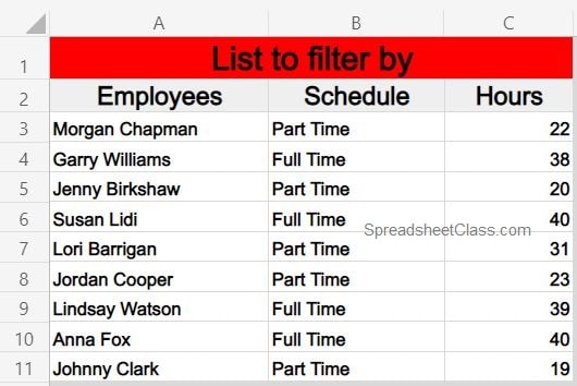
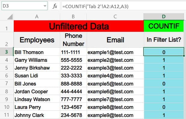
In this example, we have a set of data that shows a list of employees within an individual department at a company, as well as their contact information. We also have another list that shows employees within the department who are eligible for a bonus.

We are going to filter the data set that shows employees and their contact information, by the list of eligible employees… so that only the contact information data of eligible employees is displayed in the filter output.

The task: Show employee contact information for employees who are eligible for a bonus

The logic: In column D, use the COUNTIF function to check whether the names in column A are contained in the list to filter by in the range F3:F17. Filter the range A3:C17, where the values in the range D3:D17 are equal to 1.

The formulas: The COUNTIF formula below, is entered in cell D3, and is copied into the cells below it to fill column D. The FILTER formula below is entered in cell H3.

=COUNTIF(F2:F12,A3)

=FILTER(A3:C17,D3:D17=1)

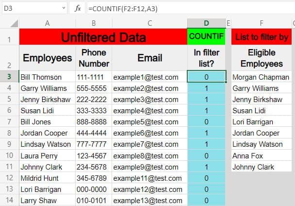
As shown in the example above, column D is being used as a place for the COUNTIF function to provide a simple indication of whether each name in column A is found within the «list to filter by» in column F.

If the name is found in the list the cell will display the number 1, and if it is not found in the list the cell will display the number 0.

This allows you to use column D as the criteria for the filter function, where you can simply tell Excel via the FILTER function to show only the rows where column D is equal to 1 (as shown below).

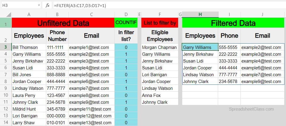
Now the filtered results in columns H through I only show the rows containing names / employees who are on the eligibility list.

Filter based on a list in Excel, where the criteria is NOT found in list

So in this example, let’s say that we want to use the same data / list to filter by as the previous example, but in this case we want to show only the rows where the name is NOT in the eligibility list. In other words we will display a list of employees who are NOT eligible for a bonus.

You might have already recognized that you can do this by changing the filter criteria from «=1» to «=0». This will definitely work, but you might not always be dealing with numbers as a part of your FILTER formula criteria, and so if you ever need to filter rows where NOT equal to a certain string of text, you’ll need to know how to use the «Not equal to» operator / sign in Excel.

The «Not equal to» sign in Excel is expressed like this <>, which is a «less than» symbol followed by a «greater than» symbol. We will use this below to display only rows that are not equal to 1.

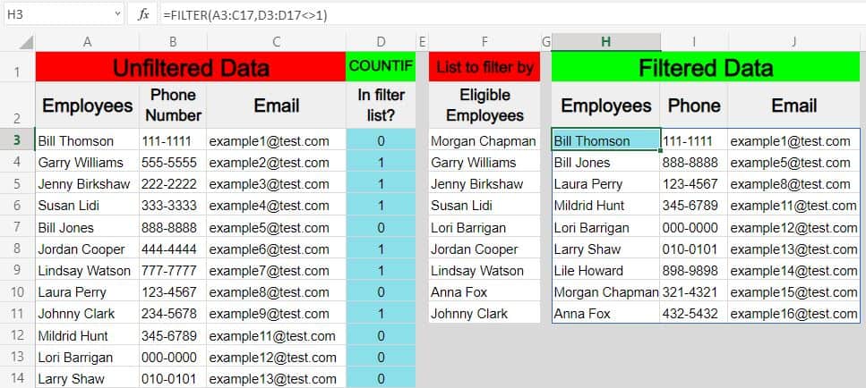
The task: Show employee contact information for employees who are NOT eligible for a bonus

The formulas: The COUNTIF formula below, is entered in cell D3, and is copied into the cells below it to fill column D. The FILTER formula below is entered in cell H3.

=COUNTIF(F2:F12,A3)

=FILTER(A3:C17,D3:D17<>1)

Filtering by a list when the data is on separate sheets

Now that you know how to filter by a list where all of the data and the formula are held on the same sheet/tab, let’s go over how to filter by a list when using multiple tabs.

There are a variety of arrangements that are possible when using multiple tabs for filtering a range by an array, and so I’ll go over each of them.

In the examples below, both the unfiltered source data (data to be filtered) and the list to filter by are given in the format of multiple column ranges. In other words, the list that we want to filter by is provided with other columns of data beside it this time. This will not change how we setup the formula, but it is important to learn how to identify your column references with data that looks like this.

This type of situation where the list to filter by is attached to other data can be expected in the real world… but it presents another potentially confusing situation with setting up your formula references because of the added columns. i.e. It’s easier to identify the list to filter by when the list is just a single column.

Again, if you are setting up a formula and you find yourself confused, first determine which data needs to be filtered, and which data you are using to filter with/by, then use the COUNTIF with the FILTER function as explained in this lesson.

Source data and formula on the same sheet

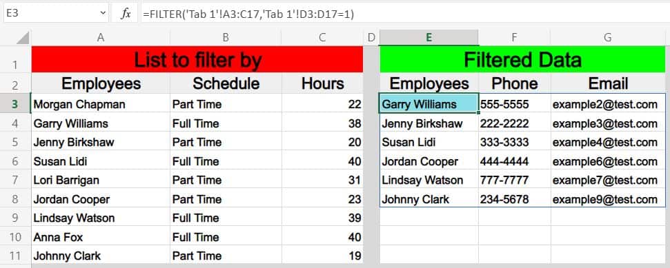
Here is an example showing how to set up your formula when the unfiltered source data and filter formula are on the same tab… but where your list that you want to filter by is on a separate tab.

Unfiltered source data & COUNTIF function: Tab 1

FILTER formula: Tab 1

List to filter by: Tab 2

The formulas: The COUNTIF formula below, is entered in cell D3 of Tab 1, and is copied into the cells below it to fill column D. The FILTER formula below is entered in cell F3 of Tab 1.

=COUNTIF(‘Tab 2’!A2:A12,A3)

=FILTER(A3:C17,D3:D17=1)

The list that you will use as the criteria in this example is on it’s own tab, as shown above.

Directly below is the «Unfiltered Data». As you can see the COUNTIF function is being used like in the previous examples, to provide a clear indication of whether or not each row in the unfiltered data should appear in the filter results (Whether or not the name in column A is found in the «List to filter by»).

List to filter by and formula on the same sheet

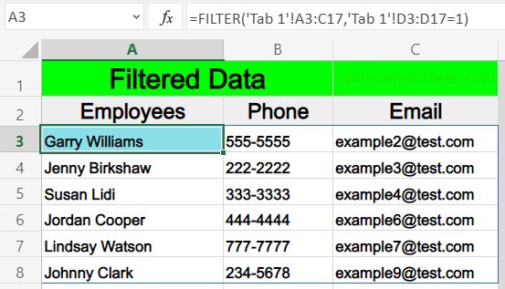
Here is an example showing how to set up your formula when the list that you want to filter by and the formula are on the same tab, but the unfiltered source data is on a separate tab.

Unfiltered source data & COUNTIF function: Tab 1

List to filter by: Tab 2

FILTER formula: Tab 2

The formulas: The COUNTIF formula below, is entered in cell D3 on Tab 1, and is copied into the cells below it to fill column D. The FILTER formula below is entered in cell E3 in Tab 2.

=COUNTIF(‘Tab 2’!A2:A12,A3)

=FILTER(‘Tab 1′!A3:C17,’Tab 1’!D3:D17=1)

Source data, list to filter by, and formula, all on separate sheets

Finally, here is an example showing how to set up your formula when the unfiltered source data (data to be filtered), the list to filter by, and the formula are each on a separate tab.

Unfiltered source data / COUNTIF function: Tab 1

List to filter by: Tab 2

FILTER formula: Tab 3

The formulas: The COUNTIF formula below, is entered in cell D3 in Tab 1, and is copied into the cells below it to fill column D. The FILTER formula below is entered in cell H3 in Tab 3.

=COUNTIF(‘Tab 2’!A2:A12,A3)

=FILTER(‘Tab 1′!A3:C17,’Tab 1’!D3:D17=1)

Pop Quiz: Test your knowledge

Answer the questions below about filtering based on a list, to refine your knowledge! Scroll to the very bottom to find the answers to the quiz.

Question #1

Which of the following formulas has a criteria range of C3:C10?

=FILTER(A3:C10,D3:D10=1)
=FILTER(A3:C10,C3:C10=1)
=FILTER(C3:C10,D3:D10=1)

Question #2

Which of the following formulas has a source range of A3:G?

=FILTER(C3:C10,G3:G10=1)
=FILTER(A3:C10,A3:A10=1)
=FILTER(A3:G10,D3:D10=1)

Question #3

True or False: The COUNTIF function can be used to create a «Criteria column» for the FILTER function.

True
False

Answers to the questions above:

Question 1: 2

Question 2: 3

Question 3: 1

Источник

Excel has many functions where a user needs to specify a single or multiple criteria to get the result. For example, if you want to count cells based on multiple criteria, you can use the COUNTIF or COUNTIFS functions in Excel.

This tutorial covers various ways of using a single or multiple criteria in COUNTIF and COUNTIFS function in Excel.

While I will primarily be focussing on COUNTIF and COUNTIFS functions in this tutorial, all these examples can also be used in other Excel functions that take multiple criteria as inputs (such as SUMIF, SUMIFS, AVERAGEIF, and AVERAGEIFS).

An Introduction to Excel COUNTIF and COUNTIFS Functions
- Excel COUNTIF Function (takes Single Criteria)
- Excel COUNTIFS Function (takes Multiple Criteria)
Using NUMBER Criteria in Excel COUNTIF Functions
- #1 Count Cells when Criteria is EQUAL to a Value
- #2 Count Cells when Criteria is GREATER THAN a Value
- #3 Count Cells when Criteria is LESS THAN a Value
- #4 Count Cells with Multiple Criteria – Between Two Values
Using TEXT Criteria in Excel Functions
- #1 Count Cells when Criteria is EQUAL to a Specified text
- #2 Count Cells when Criteria is NOT EQUAL to a Specified text
Using DATE Criteria in Excel COUNTIF and COUNTIFS Functions
- #1 Count Cells when Criteria is EQUAL to a Specified Date
- #2 Count Cells when Criteria is BEFORE or AFTER to a Specified Date
- #3 Count Cells with Multiple Criteria – Between Two Dates
Using WILDCARD CHARACTERS in Criteria in COUNTIF & COUNTIFS Functions
- #1 Count Cells that contain Text
- #2 Count Non-blank Cells
- #3 Count Cells that contain specific text

An Introduction to Excel COUNTIF and COUNTIFS Functions

Let’s first get a grip on using COUNTIF and COUNTIFS functions in Excel.

Excel COUNTIF Function (takes Single Criteria)

Excel COUNTIF function is best suited for situations when you want to count cells based on a single criterion. If you want to count based on multiple criteria, use COUNTIFS function.

Syntax

=COUNTIF(range, criteria)

Input Arguments

range – the range of cells which you want to count.
criteria – the criteria that must be evaluated against the range of cells for a cell to be counted.

Excel COUNTIFS Function (takes Multiple Criteria)

Excel COUNTIFS function is best suited for situations when you want to count cells based on multiple criteria.

Syntax

=COUNTIFS(criteria_range1, criteria1, [criteria_range2, criteria2]…)

Input Arguments

criteria_range1 – The range of cells for which you want to evaluate against criteria1.
criteria1 – the criteria which you want to evaluate for criteria_range1 to determine which cells to count.
[criteria_range2] – The range of cells for which you want to evaluate against criteria2.
[criteria2] – the criteria which you want to evaluate for criteria_range2 to determine which cells to count.

Now let’s have a look at some examples of using multiple criteria in COUNTIF functions in Excel.

Using NUMBER Criteria in Excel COUNTIF Functions

#1 Count Cells when Criteria is EQUAL to a Value

To get the count of cells where the criteria argument is equal to a specified value, you can either directly enter the criteria or use the cell reference that contains the criteria.

Below is an example where we count the cells that contain the number 9 (which means that the criteria argument is equal to 9). Here is the formula:

=COUNTIF($B$2:$B$11,D3)

In the above example (in the pic), the criteria is in cell D3. You can also enter the criteria directly into the formula. For example, you can also use:

=COUNTIF($B$2:$B$11,9)

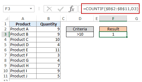
#2 Count Cells when Criteria is GREATER THAN a Value

To get the count of cells with a value greater than a specified value, we use the greater than operator (“>”). We could either use it directly in the formula or use a cell reference that has the criteria.

Whenever we use an operator in criteria in Excel, we need to put it within double quotes. For example, if the criteria is greater than 10, then we need to enter “>10” as the criteria (see pic below):

Here is the formula:

=COUNTIF($B$2:$B$11,”>10″)

You can also have the criteria in a cell and use the cell reference as the criteria. In this case, you need NOT put the criteria in double quotes:

=COUNTIF($B$2:$B$11,D3)

There could also be a case when you want the criteria to be in a cell, but don’t want it with the operator. For example, you may want the cell D3 to have the number 10 and not >10.

In that case, you need to create a criteria argument which is a combination of operator and cell reference (see pic below):

=COUNTIF($B$2:$B$11,”>”&D3)

NOTE: When you combine an operator and a cell reference, the operator is always in double quotes. The operator and cell reference are joined by an ampersand (&).

#3 Count Cells when Criteria is LESS THAN a Value

To get the count of cells with a value less than a specified value, we use the less than operator (“<“). We could either use it directly in the formula or use a cell reference that has the criteria.

Whenever we use an operator in criteria in Excel, we need to put it within double quotes. For example, if the criterion is that the number should be less than 5, then we need to enter “<5” as the criteria (see pic below):

=COUNTIF($B$2:$B$11,”<5″)

You can also have the criteria in a cell and use the cell reference as the criteria. In this case, you need NOT put the criteria in double quotes (see pic below):

=COUNTIF($B$2:$B$11,D3)

Also, there could be a case when you want the criteria to be in a cell, but don’t want it with the operator. For example, you may want the cell D3 to have the number 5 and not <5.

In that case, you need to create a criteria argument which is a combination of operator and cell reference:

=COUNTIF($B$2:$B$11,”<“&D3)

NOTE: When you combine an operator and a cell reference, the operator is always in double quotes. The operator and cell reference are joined by an ampersand (&).

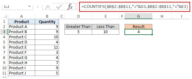
#4 Count Cells with Multiple Criteria – Between Two Values

To get a count of values between two values, we need to use multiple criteria in the COUNTIF function.

Here are two methods of doing this:

METHOD 1: Using COUNTIFS function

COUNTIFS function can handle multiple criteria as arguments and counts the cells only when all the criteria are TRUE. To count cells with values between two specified values (say 5 and 10), we can use the following COUNTIFS function:

=COUNTIFS($B$2:$B$11,”>5″,$B$2:$B$11,”<10″)

NOTE: The above formula does not count cells that contain 5 or 10. If you want to include these cells, use greater than equal to (>=) and less than equal to (<=) operators. Here is the formula:

=COUNTIFS($B$2:$B$11,”>=5″,$B$2:$B$11,”<=10″)

You can also have these criteria in cells and use the cell reference as the criteria. In this case, you need NOT put the criteria in double quotes (see pic below):

You can also use a combination of cells references and operators (where the operator is entered directly in the formula). When you combine an operator and a cell reference, the operator is always in double quotes. The operator and cell reference are joined by an ampersand (&).

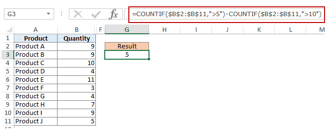
METHOD 2: Using two COUNTIF functions

If you have multiple criteria, you can either use COUNTIFS or create a combination of COUNTIF functions. The formula below would also do the same thing:

=COUNTIF($B$2:$B$11,”>5″)-COUNTIF($B$2:$B$11,”>10″)

In the above formula, we first find the number of cells that have a value greater than 5 and we subtract the count of cells with a value greater than 10. This would give us the result as 5 (which is the number of cells that have values more than 5 and less than equal to 10).

If you want the formula to include both 5 and 10, use the following formula instead:

=COUNTIF($B$2:$B$11,”>=5″)-COUNTIF($B$2:$B$11,”>10″)

If you want the formula to exclude both ‘5’ and ’10’ from the counting, use the following formula:

=COUNTIF($B$2:$B$11,”>=5″)-COUNTIF($B$2:$B$11,”>10″)-COUNTIF($B$2:$B$11,10)

You can have these criteria in cells and use the cells references, or you can use a combination of operators and cells references.

Using TEXT Criteria in Excel Functions

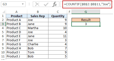
#1 Count Cells when Criteria is EQUAL to a Specified text

To count cells that contain an exact match of the specified text, we can simply use that text as the criteria. For example, in the dataset (shown below in the pic), if I want to count all the cells with the name Joe in it, I can use the below formula:

=COUNTIF($B$2:$B$11,”Joe”)

Since this is a text string, I need to put the text criteria in double quotes.

You can also have the criteria in a cell and then use that cell reference (as shown below):

=COUNTIF($B$2:$B$11,E3)

NOTE: You can get wrong results if there are leading/trailing spaces in the criteria or criteria range. Make sure you clean the data before using these formulas.

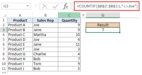
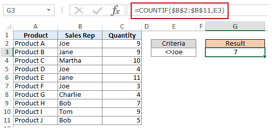
#2 Count Cells when Criteria is NOT EQUAL to a Specified text

Similar to what we saw in the above example, you can also count cells that do not contain a specified text. To do this, we need to use the not equal to operator (<>).

Suppose you want to count all the cells that do not contain the name JOE, here is the formula that will do it:

=COUNTIF($B$2:$B$11,”<>Joe”)

You can also have the criteria in a cell and use the cell reference as the criteria. In this case, you need NOT put the criteria in double quotes (see pic below):

=COUNTIF($B$2:$B$11,E3)

There could also be a case when you want the criteria to be in a cell but don’t want it with the operator. For example, you may want the cell D3 to have the name Joe and not <>Joe.

In that case, you need to create a criteria argument which is a combination of operator and cell reference (see pic below):

=COUNTIF($B$2:$B$11,”<>”&E3)

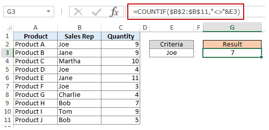
When you combine an operator and a cell reference, the operator is always in double quotes. The operator and cell reference are joined by an ampersand (&).

Using DATE Criteria in Excel COUNTIF and COUNTIFS Functions

Excel store date and time as numbers. So we can use it the same way we use numbers.

#1 Count Cells when Criteria is EQUAL to a Specified Date

To get the count of cells that contain the specified date, we would use the equal to operator (=) along with the date.

To use the date, I recommend using the DATE function, as it gets rid of any possibility of error in the date value. So, for example, if I want to use the date September 1, 2015, I can use the DATE function as shown below:

=DATE(2015,9,1)

This formula would return the same date despite regional differences. For example, 01-09-2015 would be September 1, 2015 according to the US date syntax and January 09, 2015 according to the UK date syntax. However, this formula would always return September 1, 2105.

Here is the formula to count the number of cells that contain the date 02-09-2015:

=COUNTIF($A$2:$A$11,DATE(2015,9,2))

#2 Count Cells when Criteria is BEFORE or AFTER to a Specified Date

To count cells that contain date before or after a specified date, we can use the less than/greater than operators.

For example, if I want to count all the cells that contain a date that is after September 02, 2015, I can use the formula:

=COUNTIF($A$2:$A$11,”>”&DATE(2015,9,2))

Similarly, you can also count the number of cells before a specified date. If you want to include a date in the counting, use and ‘equal to’ operator along with ‘greater than/less than’ operator.

You can also use a cell reference that contains a date. In this case, you need to combine the operator (within double quotes) with the date using an ampersand (&).

See example below:

=COUNTIF($A$2:$A$11,”>”&F3)

#3 Count Cells with Multiple Criteria – Between Two Dates

To get a count of values between two values, we need to use multiple criteria in the COUNTIF function.

We can do this using two methods – One single COUNTIFS function or two COUNTIF functions.

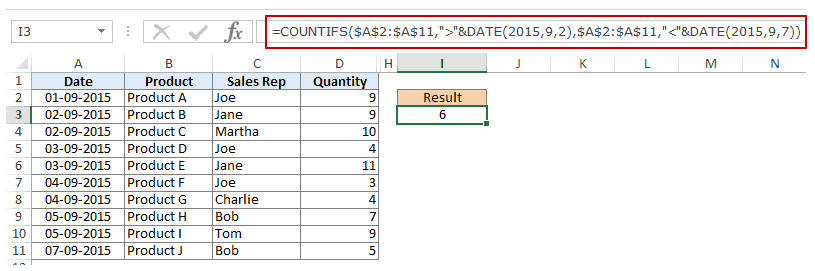
METHOD 1: Using COUNTIFS function

COUNTIFS function can take multiple criteria as the arguments and counts the cells only when all the criteria are TRUE. To count cells with values between two specified dates (say September 2 and September 7), we can use the following COUNTIFS function:

=COUNTIFS($A$2:$A$11,”>”&DATE(2015,9,2),$A$2:$A$11,”<“&DATE(2015,9,7))

The above formula does not count cells that contain the specified dates. If you want to include these dates as well, use greater than equal to (>=) and less than equal to (<=) operators. Here is the formula:

=COUNTIFS($A$2:$A$11,”>=”&DATE(2015,9,2),$A$2:$A$11,”<=”&DATE(2015,9,7))

You can also have the dates in a cell and use the cell reference as the criteria. In this case, you can not have the operator with the date in the cells. You need to manually add operators in the formula (in double quotes) and add cell reference using an ampersand (&). See the pic below:

=COUNTIFS($A$2:$A$11,”>”&F3,$A$2:$A$11,”<“&G3)

METHOD 2: Using COUNTIF functions

If you have multiple criteria, you can either use one COUNTIFS function or create a combination of two COUNTIF functions. The formula below would also do the trick:

=COUNTIF($A$2:$A$11,”>”&DATE(2015,9,2))-COUNTIF($A$2:$A$11,”>”&DATE(2015,9,7))

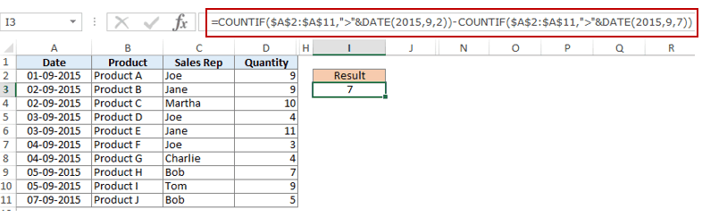
In the above formula, we first find the number of cells that have a date after September 2 and we subtract the count of cells with dates after September 7. This would give us the result as 7 (which is the number of cells that have dates after September 2 and on or before September 7).

If you don’t want the formula to count both September 2 and September 7, use the following formula instead:

=COUNTIF($A$2:$A$11,”>=”&DATE(2015,9,2))-COUNTIF($A$2:$A$11,”>”&DATE(2015,9,7))

If you want to exclude both the dates from counting, use the following formula:

=COUNTIF($A$2:$A$11,”>”&DATE(2015,9,2))-COUNTIF($A$2:$A$11,”>”&DATE(2015,9,7)-COUNTIF($A$2:$A$11,DATE(2015,9,7)))

Also, you can have the criteria dates in cells and use the cells references (along with operators in double quotes joined using ampersand).

Using WILDCARD CHARACTERS in Criteria in COUNTIF & COUNTIFS Functions

There are three wildcard characters in Excel:

* (asterisk) – It represents any number of characters. For example, ex* could mean excel, excels, example, expert, etc.
? (question mark) – It represents one single character. For example, Tr?mp could mean Trump or Tramp.
~ (tilde) – It is used to identify a wildcard character (~, *, ?) in the text.

You can use COUNTIF function with wildcard characters to count cells when other inbuilt count function fails. For example, suppose you have a data set as shown below:

Now let’s take various examples:

#1 Count Cells that contain Text

To count cells with text in it, we can use the wildcard character * (asterisk). Since asterisk represents any number of characters, it would count all cells that have any text in it. Here is the formula:

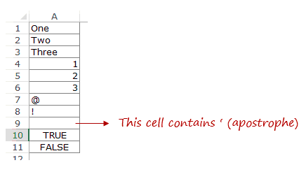
=COUNTIFS($C$2:$C$11,”*”)

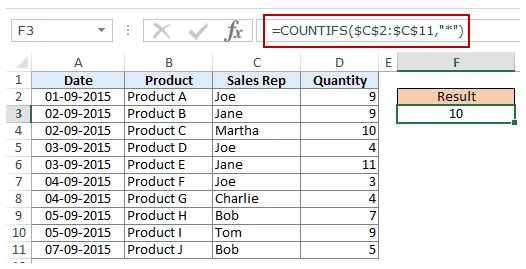
Note: The formula above ignores cells that contain numbers, blank cells, and logical values, but would count the cells contain an apostrophe (and hence appear blank) or cells that contain empty string (=””) which may have been returned as a part of a formula.

Here is a detailed tutorial on handling cases where there is an empty string or apostrophe.

Here is a detailed tutorial on handling cases where there are empty strings or apostrophes.

Below is a video that explains different scenarios of counting cells with text in it.

#2 Count Non-blank Cells

If you are thinking of using COUNTA function, think again.

Try it and it might fail you. COUNTA will also count a cell that contains an empty string (often returned by formulas as =”” or when people enter only an apostrophe in a cell). Cells that contain empty strings look blank but are not, and thus counted by the COUNTA function.

COUNTA will also count a cell that contains an empty string (often returned by formulas as =”” or when people enter only an apostrophe in a cell). Cells that contain empty strings look blank but are not, and thus counted by the COUNTA function.

So if you use the formula =COUNTA(A1:A11), it returns 11, while it should return 10.

Here is the fix:

=COUNTIF($A$1:$A$11,”?*”)+COUNT($A$1:$A$11)+SUMPRODUCT(–ISLOGICAL($A$1:$A$11))

Let’s understand this formula by breaking it down:

#3 Count Cells that contain specific text

Let’s say we want to count all the cells where the sales rep name begins with J. This can easily be achieved by using a wildcard character in COUNTIF function. Here is the formula:

=COUNTIFS($C$2:$C$11,”J*”)

The criteria J* specifies that the text in a cell should begin with J and can contain any number of characters.

If you want to count cells that contain the alphabet anywhere in the text, flank it with an asterisk on both sides. For example, if you want to count cells that contain the alphabet “a” in it, use *a* as the criteria.

This article is unusually long compared to my other articles. Hope you have enjoyed it. Let me know your thoughts by leaving a comment.

You May Also Find the following Excel tutorials useful:

Count the number of words in Excel.
Count Cells Based on Background Color in Excel.
How to Sum a Column in Excel (5 Really Easy Ways)

Источник