
Create a simple formula in Excel
Excel for Microsoft 365 Excel for Microsoft 365 for Mac Excel 2021 Excel 2021 for Mac Excel 2019 Excel 2019 for Mac Excel 2016 Excel 2016 for Mac Excel 2013 Excel 2010 Excel 2007 Excel for Mac 2011 More…Less
You can create a simple formula to add, subtract, multiply or divide values in your worksheet. Simple formulas always start with an equal sign (=), followed by constants that are numeric values and calculation operators such as plus (+), minus (—), asterisk(*), or forward slash (/) signs.
Let’s take an example of a simple formula.
-
On the worksheet, click the cell in which you want to enter the formula.
-
Type the = (equal sign) followed by the constants and operators (up to 8192 characters) that you want to use in the calculation.
For our example, type =1+1.
Notes:
-
Instead of typing the constants into your formula, you can select the cells that contain the values that you want to use and enter the operators in between selecting cells.
-
Following the standard order of mathematical operations, multiplication and division is performed before addition and subtraction.
-
-
Press Enter (Windows) or Return (Mac).
Let’s take another variation of a simple formula. Type =5+2*3 in another cell and press Enter or Return. Excel multiplies the last two numbers and adds the first number to the result.
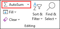
Use AutoSum
You can use AutoSum to quickly sum a column or row or numbers. Select a cell next to the numbers you want to sum, click AutoSum on the Home tab, press Enter (Windows) or Return (Mac), and that’s it!
When you click AutoSum, Excel automatically enters a formula (that uses the SUM function) to sum the numbers.
Note: You can also type ALT+= (Windows) or ALT+ += (Mac) into a cell, and Excel automatically inserts the SUM function.
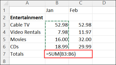
Here’s an example. To add the January numbers in this Entertainment budget, select cell B7, the cell immediately below the column of numbers. Then click AutoSum. A formula appears in cell B7, and Excel highlights the cells you’re totaling.
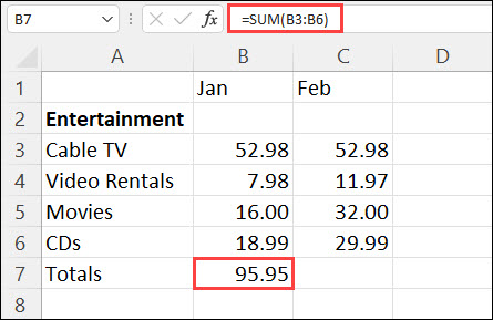
Press Enter to display the result (95.94) in cell B7. You can also see the formula in the formula bar at the top of the Excel window.
Notes:
-
To sum a column of numbers, select the cell immediately below the last number in the column. To sum a row of numbers, select the cell immediately to the right.
-
Once you create a formula, you can copy it to other cells instead of typing it over and over. For example, if you copy the formula in cell B7 to cell C7, the formula in C7 automatically adjusts to the new location, and calculates the numbers in C3:C6.
-
You can also use AutoSum on more than one cell at a time. For example, you could highlight both cell B7 and C7, click AutoSum, and total both columns at the same time.
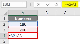
Copy the example data in the following table, and paste it in cell A1 of a new Excel worksheet. If you need to, you can adjust the column widths to see all the data.
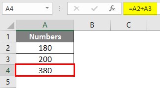
Note: For formulas to show results, select them, press F2, and then press Enter (Windows) or Return (Mac).
|
Data |
||
|
2 |
||
|
5 |
||
|
Formula |
Description |
Result |
|
=A2+A3 |
Adds the values in cells A1 and A2 |
=A2+A3 |
|
=A2-A3 |
Subtracts the value in cell A2 from the value in A1 |
=A2-A3 |
|
=A2/A3 |
Divides the value in cell A1 by the value in A2 |
=A2/A3 |
|
=A2*A3 |
Multiplies the value in cell A1 times the value in A2 |
=A2*A3 |
|
=A2^A3 |
Raises the value in cell A1 to the exponential value specified in A2 |
=A2^A3 |
|
Formula |
Description |
Result |
|
=5+2 |
Adds 5 and 2 |
=5+2 |
|
=5-2 |
Subtracts 2 from 5 |
=5-2 |
|
=5/2 |
Divides 5 by 2 |
=5/2 |
|
=5*2 |
Multiplies 5 times 2 |
=5*2 |
|
=5^2 |
Raises 5 to the 2nd power |
=5^2 |
Need more help?
You can always ask an expert in the Excel Tech Community or get support in the Answers community.
Need more help?
Excel is full of formulas. Those who master those formulas are pros of Excel. However, at the start of learning Excel, everyone is curious to know how to apply or create formulas in Excel. If you are one of them who is willing to learn how to create formulas in Excel, then this article is best suited for you. This article will have a complete guide from zero to intermediate level formula application in Excel.
Let us create a simple calculator-type formula for adding up numbers to start with Excel formulas.
You can download this Create a Formula Excel Template here – Create a Formula Excel Template
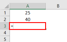
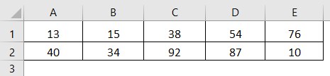
Look at the below data of numbers.
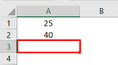
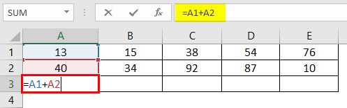
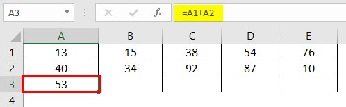
In cell A1, we have 25. The A2 cell has 40, the number.
In cell A3, we need the summation of these two numbers.
In Excel, to start the formula, always put the equal sign first.
Now, insert 25 + 40 as the equation.
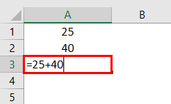
It is very similar to what we do in the calculator.
Press the “Enter” key to get the total of these numbers.

So, 25 + 40 is 65, the same we got in cell A3.
Table of contents
- How to Create a Formula in Excel?
- #1 Create Formula Flexible with Cell References
- #2 Use SUM Function to Add Up Numbers
- #3 Create Formula References to Other Cells Excel
- Recommended Articles
#1 Create Formula Flexible with Cell References
Let us start.
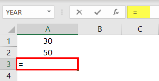
- From the above example, we will change the number from 25 to 30 and 40 to 50.

Even though we have changed numbers in cells A1 and A2, our formula only shows the old result of 65. It is a problem with direct numbers passing to the formula. It does not make the formula flexible enough to update the new result.
- We can give cell reference as the formula reference to overcoming this issue. For example, open the equal sign in cell A3.

- Then, select cell A1.

- Insert plus (+) sign and select cell A2.

- Press the “Enter” key to get the result.


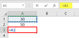
As we can see in the formula bar, it is not showing the result. Rather, it shows the formula itself, and cell A3 shows the result of the formula.
Now, we can change the numbers in A1 and A2 cells to see the immediate impact of the formula.
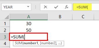
#2 Use SUM Function to Add Up Numbers
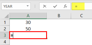
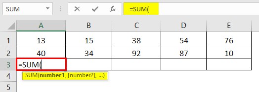
To get used to the formulas in Excel, let us start with the simple SUM function. All the formulas should begin with “+” or “=.” So, open the equal sign in cell A3.
Start typing the SUM to see the intellisense list of Excel functionsExcel functions help the users to save time and maintain extensive worksheets. There are 100+ excel functions categorized as financial, logical, text, date and time, Lookup & Reference, Math, Statistical and Information functions.read more.
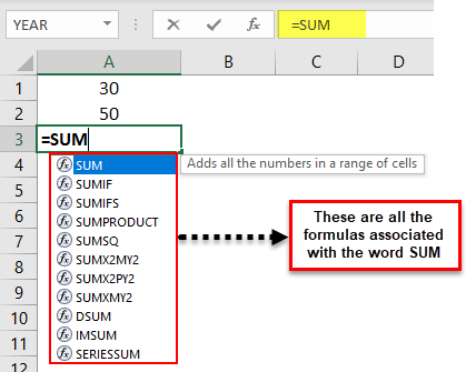
Press the “Tab” key once the SUM formula is selected to open the SUM function in excel.The SUM function in excel adds the numerical values in a range of cells. Being categorized under the Math and Trigonometry function, it is entered by typing “=SUM” followed by the values to be summed. The values supplied to the function can be numbers, cell references or ranges.read more
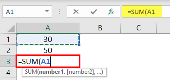
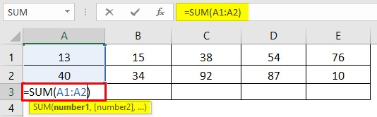
The first argument of the SUM function is Number 1, whichis the first number we need to add. In this example, cell A1. So, we must select cell A1.
The next argument is Number 2, the second number or item we need to add, A2 cell.
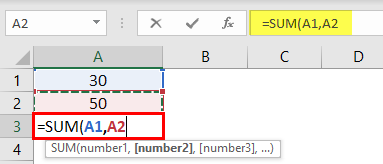
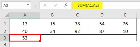
Now, we must close the bracket and press the “Enter” key to see the result of the SUM function.
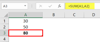
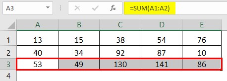
Like this, we can create simple formulas in Excel to do the calculations.
#3 Create Formula References to Other Cells Excel
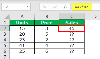
We have seen the basics of creating a formula in Excel. Similarly, we can apply one formula to other related cells as well. For example, look at the below data.
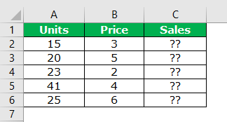
In column A we have “Units.” In column B, we have the “Price Per Unit.”
In the column, C needs to arrive at “Sales Amount.” For arriving at the sales amount, the formula is Units * Price.
- So, we must open an equal sign in cell C2.
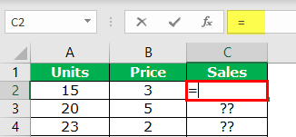
- Select cell A2 (units).
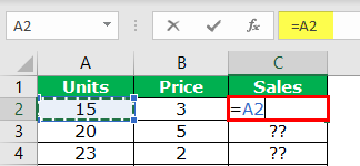
- Enter multiple sign (*) and select the B2 cell (price).
- Press the “Enter” key to get the sales amount.
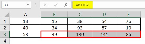
Now, we have applied the formula in cell C2. How about the remaining cells?
Can you enter the same formula for the remaining cells individually?
If you think that way, you will be delighted to hear that the “formula is to be applied to a single cell, then we can copy-paste to other cells.”
Now first, look at the formula we have applied.
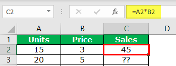
The formula says A2 * B2.
So, when we copy and paste the formula below, cell A2 becomes A3, and B2 becomes B3.
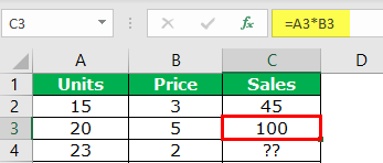
Similarly, row numbers keep changing as we move down, and column letters will also change if we move either left or right.
- Copy and paste the formula to other cells to result in all the cells.
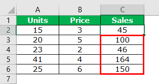
Like this, we can create a simple formula in Excel to start your learning.
Recommended Articles
This article has been a guide to creating a formula in Excel. Here, we learn to create a simple Excel formula and practical examples, and a downloadable template. You may learn more about Excel from the following articles: –
- Write Formula in Excel
- PI in Excel
- Excel Formula Not Working
- List of Basic Excel Formulas
How to Create a Formula in Excel: Beginner Tutorial (2023)
Excel is all about running calculations! And so creating and operating a formula in Excel is simple.
An Excel formula is a combination of operators and operands. For example, 2 + 2 = 4 is a formula where 2s are the operands, plus sign (+) is the operator, and 4 is the answer to the formula.
Only if you know the basics to write a formula in Excel – there’s a high chance you’d solve most of your Excel problems. This article explains the basics of creating Excel formulas.
So let’s dive right in.
As you scroll down, download our free sample workbook here to practice the examples used in the guide below. 😀
How to create formulas in Excel
Creating Excel formulas is easy as pie.
For example, what is 10 divided by 2? Can you calculate this in Excel?
1. Start by activating a cell.
2. Write an equal sign.

It is very important to start any formula with an equal sign. If you do not start with an equal sign, Excel wouldn’t recognize it as a formula but as a text string.
3. Input the simple mathematical operation of 10 divided by 2.
= 10 / 2

4. Hit enter, and you’re good to go!

You can create the same above formula with a slight variation.
For example, if you have the operands as cell values.

1. Write the formula using cell references as follows.
= A2 / B2

The above formula translates to ‘A2 divided by A3’.
Where A2 has the numeric value 10, and A3 has the numeric value 2.
2. The results remain the same as in the above example.

Creating a formula using cell references and values
The same formula can also be created using a combination of cell references and values.
Write the following formula using cell references and values.
= A2 / 2

The above formula translates to ‘A2 divided by 2’.
Where A2 has the numeric value 10, and 2 is a value.
1. The results look as follows.

Pro Tip!
Using cell references is better than using absolute values. This is because if sometime later you change the cell value – the formula would automatically update.
How to add, subtract, multiply, and divide?
There are four basic mathematical operations – add, subtract, multiply, and divide.
Let’s now see how to perform each of these operations in Excel.
How to make a SUM formula (addition)
Adding things up in Excel can take different forms.
Excel has an in-built function for performing addition i.e. the SUM function. Here’s how you can bring it to action.
1. Write the SUM function beginning with an equal sign as follows.
= SUM (5, 5)
Every argument of the SUM function separated by a comma represents the value to be added.
Excel adds 5 into 5 to give the results below.

Easy enough? You can use the SUM function for cell references too. 🤩
2. Write the SUM function as follows.
= SUM (A2, A3)
Pro Tip!
To insert SUM from the Insert Function button, take this route.
Go to Formulas tab > Function Library > Insert function button > Type the function name.
In the Insert Function dialog box, type SUM and hit search. Select the desired function and hit ‘Okay’ to insert the same.
Excel adds the cell values of Cell A2 and Cell A3.

What makes the SUM function a big plus is its ability to add up a range of cells.
For example, see the data below.

3. To add this up in Excel using the SUM function, write the SUM function as below.
= SUM (A2:A10)

Must notice how we have defined the cell range from Cell A2 to Cell A10 as A2:A10.
4. Excel sums up all cell values in cells from A2 to A10.

You can make this function work even more interestingly by adding up multiple ranges.
5. Write the SUM function with multiple ranges as follows.
= SUM (A2:A5, B2:B8, C1:C10)


How to subtract in Excel
Subtracting in Excel is all about creating a formula with the minus sign operator (-).
For example:
1. To subtract 5 from 10, begin with an equal sign and write the following formula.
= 10 – 5
A simple subtraction formula with a minus sign operator!
Press enter and here you go.

2. Try doing the same with cell references as below.
= A2 – A3
This formula translates to A2 less A3. Where A2 has the numeric value 10, and A3 has the numeric value 5.

3. Alternatively, you can use the SUM function to perform subtraction. However, to do this you need to add a minus sign to the value to be subtracted.
= SUM (A2, -A3)
Here are the results.

How to multiply in Excel
After we have learned how to add and subtract in Excel, it’s time we learn multiplication in Excel.
First thing first, the operator for multiplication in Excel is an asterisk (*).
Now, do you remember what is 9 times 8? No?
1. Write a multiplication formula in Excel.
= 9 * 8


2. Try doing the same using cell references as below.
= A2 * A3

The formula above translates to A2 multiplied by A3.
Excel also offers an in-built function for multiplication in Excel. The PRODUCT Function!
3. Write the PRODUCT function as follows.
= PRODUCT (9, 

We have added both the values to be multiplied as the arguments to the PRODUCT function.
Here are the results.

The PRODUCT function can also find the product of multiple values (or a range of cells) at once.
For example, see the data below.

4. To multiply all these values, write the PRODUCT function as follows:
= PRODUCT (A2:A10)

Excel multiplies all the values in the specified range.

How to divide in Excel
Here comes the last operation of this guide – division. 🤞
Creating a division formula in Excel is also very straightforward.
What is the operator for division? A forward slash (/).
Also, the dividend (or the numerator) comes before the slash. And the divisor (or the denominator) comes after the slash.
1. Write a division formula as below.
= 30 / 10

Excel divides both operands to give the results as follows.

2. The same can be done using cell references.
= A2 / A3
Pro Tip!
While performing the division function in Excel, you might see the #DIV/0! Error. This error is given back by Excel when you attempt to divide the number of zero.
Basic Rule of Grade 6! No number is divisible by zero. Excel remembers that, if not us. 😆
Order of operations
Here’s an equation for you to solve.
= 2+ 4 * 6 / 3 – 2
What a mess! Which operation do you perform first?
To solve this mystery, there is an order for performing mathematical operations – PEMDAS
P = Parenthesis
E = Exponents
MD = Multiplication & Division (left to right)
AS = Addition & Subtraction
Solve the above equation in the same order, and you’d reach the answer 8.
Let Excel do the same to see the results.

Excel performs division first (6 / 3 = 2), multiplication second (4 * 2 = 8), addition third (2 + 8 = 10), and subtraction last (10 – 2 = 8), resulting in 8.
Now, let’s enclose a part of this formula in parentheses to see how the results change.
= 2+ 4 * 6 / (3 – 2)

What causes the results to change with only parenthesis added?
Excel now first performs the operation enclosed in parenthesis i.e. (3-2).
Next, multiplication is performed, then division and addition last. This causes the answer to change.
Pro Tip!
Try doing some mental maths to double-check if Excel has rightly calculated 26.
Parenthesis first = 2+ 4*6/(3 – 2)
Multiplication Second= 2+4*6/1
Division Third = 2 + 24/1
Addition Last = 2 + 24
Here’s the answer = 26
How to create formulas with references
Creating Excel formulas with references is super simple. All you need to do is replace the values in a simple formula with cell references (cells that contain those values).
For example, let’s create a multiplication formula in Excel.

Great! What if you had 2 & 4 as numerical values in cells?

Create the same formula using cell references.

You can do the same for all operators! It is this simple.
Also, what happens when a cell value changes? Until the cell reference is in place, the formula would automatically update for the cell value change.

Must note how the cell reference in the formula remains unchanged. The answer however changes as the cell value for A3 has changed.ltiple criteria lookup💡
Formulas or functions?
What is an Excel formula, and what is an Excel function? And how are these two different?
There are two ways to add 2 and 2 in Excel.
- = 2 + 2
- SUM (2,2)
The answer to them both would be the same. However, the first one is a formula created in Excel. Whereas the second one is an in-built function of Excel – the SUM function.
Functions are more like predefined formulas in Excel.
Although the function library of Microsoft Excel is huge enough for you to explore, there is a limit to it. And you may not find everything you need there.
So, you might still need to write your own formulas to perform calculations in Excel. 😉
Pro Tip!
Sometimes, you might even nest a function into a formula.
For example, what is 2 + 2 – 3?
You may write it as = (SUM (2,2)) – 3
SUM (2,2) is a function, and deducting 3 from it makes it a self-created formula.
That’s it – Now what?
Until now, we’ve created formulas using different operators, values, and cell references. And learned how to use the SUM function for addition and subtraction.
Not only that but we’ve also studied the order of operations in Excel. The above article is a whole pack of information, isn’t it?
Creating your own formulas in Excel is the first step to manipulating numbers in Excel. However, this is something very basic, and Excel has tons more to offer.
Some very important Excel functions that one must hone include the VLOOKUP, SUMIF, and IF functions.
Haven’t mastered them yet? Click here to register for my 30-minute free email course that helps you learn these and much more.
Kasper Langmann2023-02-23T14:38:38+00:00
Page load link

Spreadsheets aren’t merely for arranging data into rows and columns. Most of the time, you use them for data analysis as well.
Microsoft Excel is one of the most widely used spreadsheet applications, especially in finance and accounting. This is partly because of its easy UI and unmatched depth of functions.
In this article, you will learn:
- What Excel formulas are
- How to write a formula in Excel
- What Excel functions are
- How to work with an Excel function
- Lastly, we’ll take a look at dynamic Excel functions.
What do I need to install on my computer to follow this article?
To follow along, you will need to have Microsoft Excel installed on your computer. We’ll use a Windows computer for this article.
How can I install Microsoft Excel on my computer?
Follow these steps to install Microsoft Excel on your Windows computer:
- Sign in to www.office.com if you’re not already signed in.
- Sign in with the account associated with your Microsoft 365 subscription. You can also try out Office for free as well.
- Once signed in, select “Install Office” from the Office home page. This will automatically download Microsoft Office onto your Windows computer.
- Run the installer to set up Microsoft Office and select «Close» once you’re done.
- Once done, select the “Start” button (located at the lower-left corner of your screen) and type “Microsoft Excel.”
- Click on Microsoft Excel to open it.
- Accept the license agreement, and let’s get started.
What are Excel Formulas?
An Excel formula is an expression that carries out an operation based on the value of a cell or range of cells. You can use an Excel formula to:
- Perform simple mathematical operations such as addition or subtraction.
- Perform a simple operation like joining categorical data.
It’s important to understand two things: Excel formulas always begin with the equals «=» sign and they can return an error if not properly executed.
What Operators Are Used in Excel Formulas?
There are four different types of operators in Excel—arithmetic, comparison, text concatenation, and reference. But for most formulas, you’ll typically use these three:
Arithmetic operators
|
+ |
Addition |
|
— |
Subtraction |
|
/ |
Division |
|
* |
Multiplication |
|
^ |
Exponentiation |
Comparison operators
|
= |
Equal to |
|
> |
Greater than |
|
< |
Less than |
|
>= |
Greater than or equal to |
|
<= |
Less than or equal to |
|
<> |
Not equal to |
Text concatenation
Here you have just the ampersand “&” sign for joining text.
How Can I Create an Excel Formula?
Let’s take a simple scenario using one of the arithmetic operators.
In math, to add up two numbers, let’s say 20 and 30, you will calculate this by writing: 20 + 30 =
And this will give you 50.
In Excel, here is how it goes:
- First, open a blank Excel worksheet.
- In cell A1, type 20.
- In cell A2, type 30.
- To add it up, type in = 20 + 30 in cell A3.

5. Then, press ENTER on your keyboard. Excel will instantly calculate this and return 50.

I mentioned earlier that every formula begins with the equal «=» sign. That’s what I meant. To write a formula, you type the equal to sign followed by the numeric values. This also applies to cases of subtraction, division, multiplication, and exponentiation.
Let’s take another simple scenario using one of the comparison operators. Assume we want to find out if 30 is greater than 40.
In Excel, here is how we would do it:
- Type in =30>40
- Press ENTER.

3. This will return a FALSE because 30 isn’t greater than 40. Excel uses TRUE and FALSE for logical statements, the same way we human says yes and no.

Lastly, let’s take another simple scenario using the text concatenation operator – the ampersand “&” sign. This works with your string data types and you use it to join text.
Assume we have «Welcome», «To», and «FreeCodeCamp» all in different cells—A1, A2, and A3—of your worksheet. We would type =A1&” “&A2&” “&A3 to join them.
The space in quotes “ “ represents that we want a space between our words.

Another tip: the formula bar shows the formula used to generate a value.
What Are Excel Functions?
Excel functions are predefined inbuilt formulas that perform mathematical, statistical, and logical calculations and operations using your values and arguments.
For Excel functions, you should know that:
- They’re formulas, so yeah, they start with the equal «=» sign as well.
- The order is very important.
There are over 500 functions available. You can find all available Excel functions on the Formulas tab on the Ribbon.

But why use a function when you can just write a formula?
Here are some benefits of Excel functions.
- To improve productivity and effectiveness.
- To simplify complex calculations.
- To automate your work.
- To quickly visualize data.
What Makes Up Excel Functions?
Unlike formulas, Excel functions are made up of a structure with arguments you need to pass.
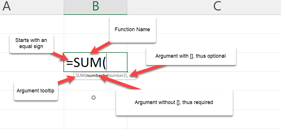
Every function:
- Starts with the equals «=» sign
- Has a name. Some examples are VLOOKUP, SUM, UNIQUE, and XLOOKUP.
- Requires arguments which are separated by commas. You should know that semicolons are used as separators in countries like Spain, France, Italy, Netherlands, and Germany. You can, however, change this via the Excel setting.
- Argument with the square brackets [] are optional
- Has an opening and closing parenthesis.
- Has an argument tooltip which shows you what you should pass.
There are some exceptions. For example,
- The DATEDIF doesn’t show in Excel because it is not a standard function and gives incorrect results in a few circumstances. However, here is the syntax:
DATEDIF(birthdate, TODAY(), "y")
- Functions like PI(), RAND(), NOW(), TODAY() require no argument.
Let’s look at a few functions:
How to Use the SUM() Function in Excel
According to the documentation, the SUM function adds values. Here is the syntax:
Let’s assume that we have a line of numbers from 1 to 10 and we want to add it up. To achieve this, we will just type =SUM(A1:A10). The A1:A10 simply returns an array of number that are situated on cell A1 to A10 which are A1, A2, and A3 up through A10.

Since the second argument is optional, that means a sum(A10) will return a value. In our case, it will return just 10 since A10 has the value 10 in it. Give it a try.
If you were writing this using the addition operator, you would have written:
=1 + 2 + 3 + 4 + 5 + 6 + 7 + 8 + 9 + 10
or
=A1 + A2 + A3 + A4 + A5 + A6 + A7 + A8 + A9 + A10
This doesn’t look very productive or efficient.
How to Use the TODAY() Function in Excel
According to the documentation, the TODAY function displays the current date on your worksheet. It also requires no argument. Here is the syntax:

Excel displays the current date automatically according to your computer’s date and time setting. The same goes for the NOW() function, which displays the current date and time.
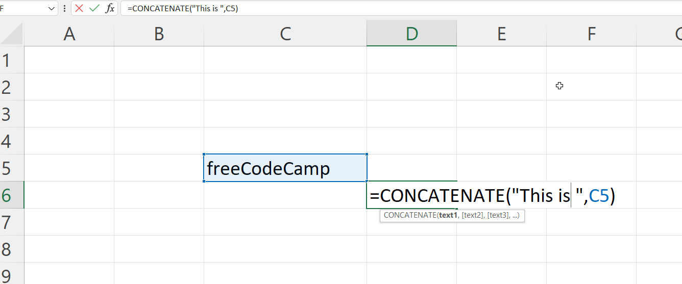
How to Use the CONCATENATE() Function in Excel
Let’s look at a text function. You use CONCATENATE to join two or more text strings into one string together.
Here is the syntax:

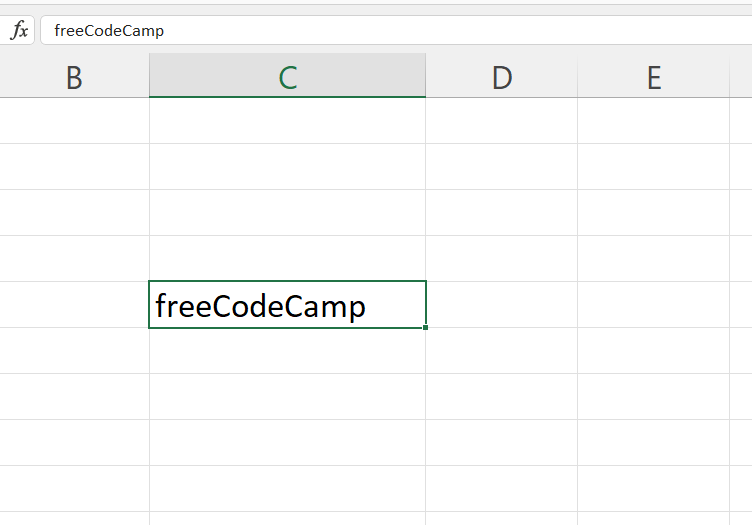
Let’s assume we want to join “This is” with “freeCodeCamp” – but in your cell, you have just «freeCodeCamp.»
If you’re going to write a string inside a formula, you must write it inside quotes like this “ “.
Why?
This way, Excel wouldnt think you’re trying to write another function.
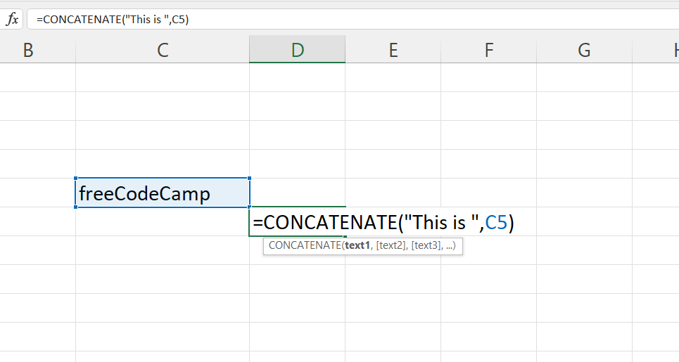
This will return the phrase “This is freeCodeCamp”
How to Use the VLOOKUP() Function in Excel
This is one of Excel’s most interesting and commonly used formulas or functions. You use it to find a value in a table or range by row.
Here is a scenario:
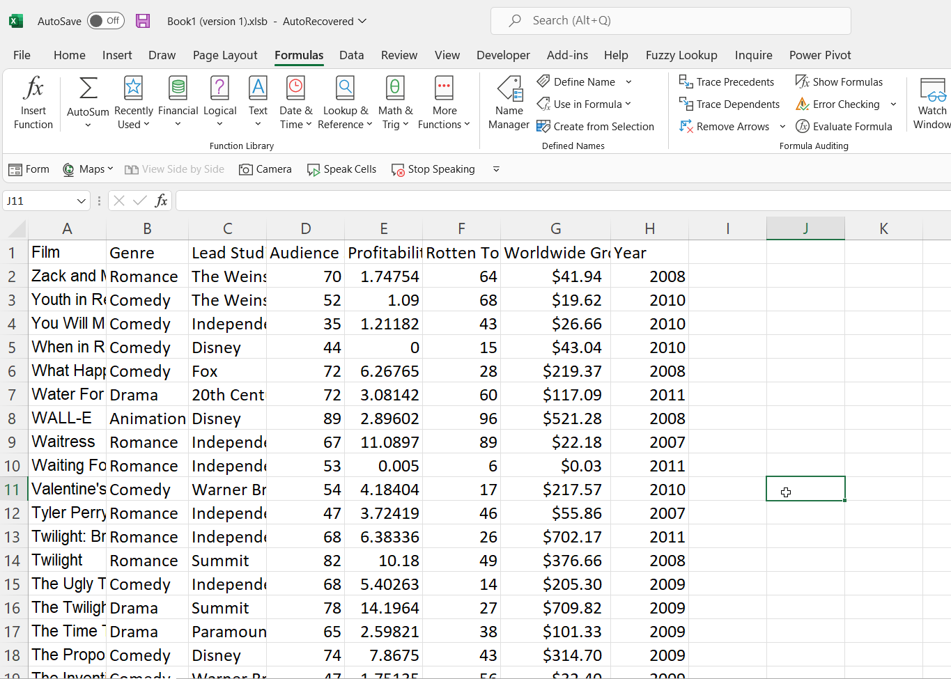
We have a simple table that shows various films along with their genre, lead studio, audience score %, profitability, rotten tomatoes %, worldwide gross and year. I would use just the first 10 rows of the sample data from this GitHub Gist.

I want that, whenever I type in a movie in the yellow cell, the year should get displayed in the green cell. Let’s use VLOOKUP to find it.
This is the VLOOKUP syntax:
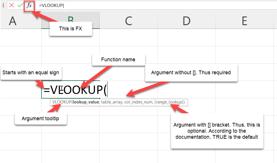
Besides writing your formulas in the cell, you can also write them using the Excel Insert Function (fx) button, which is close to the formula bar.
Let’s try this.
- Write
=Vlookup(on the green cell. - Click on fx. A dialogue box will pop up showing all the arguments this formula needs.
- Input the value for each argument.
- Lookup_value (required argument): This is what you want to find. In our case, that is the movie “Youth in Revolt” which is in cell B1.
- Table_array (required argument): This is just asking you for the table that contains the data. You give it the entire table, which in our case is A4:H13
- Col_index_num (required argument): This is asking you for the column number of the table you gave. In our case, we want the year. This is in column 8.
- Range_lookup (optional argument): Lastly, we pick if we want an approximate match (TRUE) or an exact match (FALSE).
— TRUE means approximate match, so it returns the closest or an estimate.
— FALSE means exact match, so it returns an error if it’s not found.
8. We would go for the FALSE because we want the exact match.

9. Click on «OK.» Excel will return 2010.
However, you can write this in the cell by typing in =VLOOKUP(B1,A4:H13,8,FALSE) in your cell.

Tips and Rules When Writing Excel Functions
When writing our function, Excel provides some formula tips.
- The Argument tooltip doesn’t leave until you close the last parenthesis.
- The formula bar shows your formula.
- The argument you are currently writing is always dark. Take a look at the lookup_value in the image below.
- The square brackets [] tell you it is optional.
- Lastly, the colour code – our B1 is in blue, and cell B1 is in blue to guide us on what cell or table was picked. The same thing will happen to A4:H13 when we pick it as our table_array argument.

How to Work with Nested Functions in Excel
A nested function is when you write a function within another function. For example, finding the average of the sum of values.
The first tip when writing a nested function will be to treat every function individually. So address the first function before addressing the second. A pro tip would be to look at the argument tooltip when writing it.
Let’s take a simple scenario.
We have two arrays of numbers. Each has the scores of students in the class. I want to add the two arrays before I get the average.
Let’s get started.
- Type in your = followed by the average.
- The number one will be the sum of the scores from class one.
- The number two will be the sum of the scores from class two.
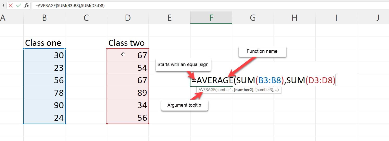

Finally, don’t forget the closing parenthesis.
Thus, the formula will be =AVERAGE(SUM(B3:B8),SUM(D3:D8)).
How to Work with Dynamic Array Functions in Excel
Dynamic array functions are formulas associated with spill array behaviour.
Before now, you wrote a function and it returned just a single input. We call these kinds of functions legacy array formulas.
Dynamic array functions, on the other hand, will return values that will enter the neighbouring cells. A few examples of dynamic array functions are:
- UNIQUE
- TEXTSPLIT
- FILTER
- SEQUENCE
- SORT
- SORTBY
- RANDARRAY
Let’s look at the UNIQUE formula.
How to Use the UNIQUE() Formula in Excel
The unique formula works by returning the unique value from an array or list. Let’s use the movie sample data from this GitHub Gist. This table contains 77 rows of film excluding the heading.

Let’s try to get the unique years from our dataset – that is, years without duplicates.
To do this:
- Type
=UNIQUE( - Select the entire array of values from the year column: =UNIQUE(H2:H78)

3. Close the parenthesis and press Enter.
Though the formula was written in a single cell, the returned value got spilled into the cells below it. That’s the spilled array behaviour.

How to Create Your Own Functions in Excel
Microsoft Excel released a bunch of new functions to make user more productive. One of these function was the LAMBDA function.
The LAMBDA function lets you create custom functions without macros, VBA or JavaScript, and reuse them throughout a workbook.
The best part? you can name it.
How to Use the LAMBDA() Function in Excel
This LAMBDA function will increase productivity by eliminating the need to copy and paste this formula, which can be error-prone.
Here is the LAMBDA syntax:
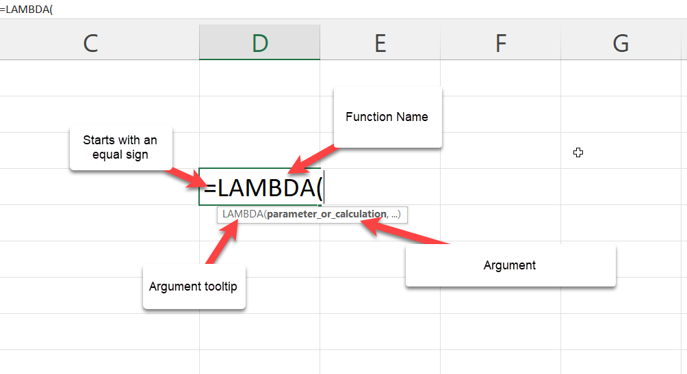
Lets start with a simple use case using the movie sample data from this GitHub Gist.
We had a column called «Worldwide Gross», lets try to find the Naira value.
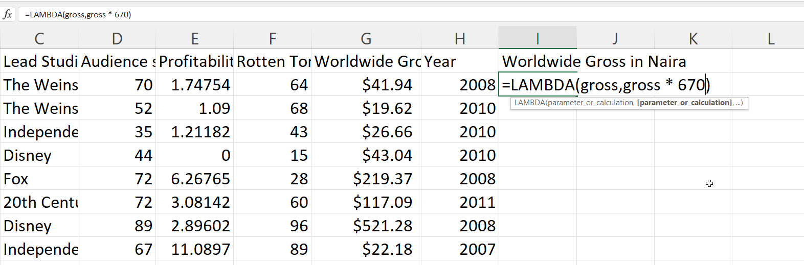
- Create a new column and call it «Worldwide Gross in Naira».
- Right below our column name, Cell I2, type
=lAMBDA( - LAMBDA requires a parameter and/or a calculation.
The parameter means the value you want to pass, in our use case we want to change the gross value. Lets call it gross.
The calculation means the formula or function you want to execute. For us, that will be to multiply it with te exchange rate. At the moment, that’s 670. so lets write gross * 670.
4. Press Enter. This will return an error because, gross doesnt exist and you need to let excel know of these names.
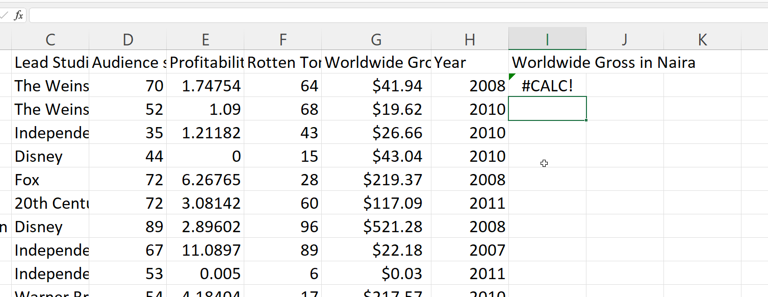
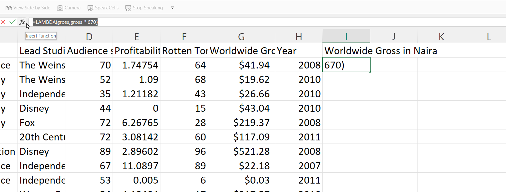
5. To make use of the newly created function, you need to copy the syntax written.
6. Go to the formula ribbon and open the name manager.
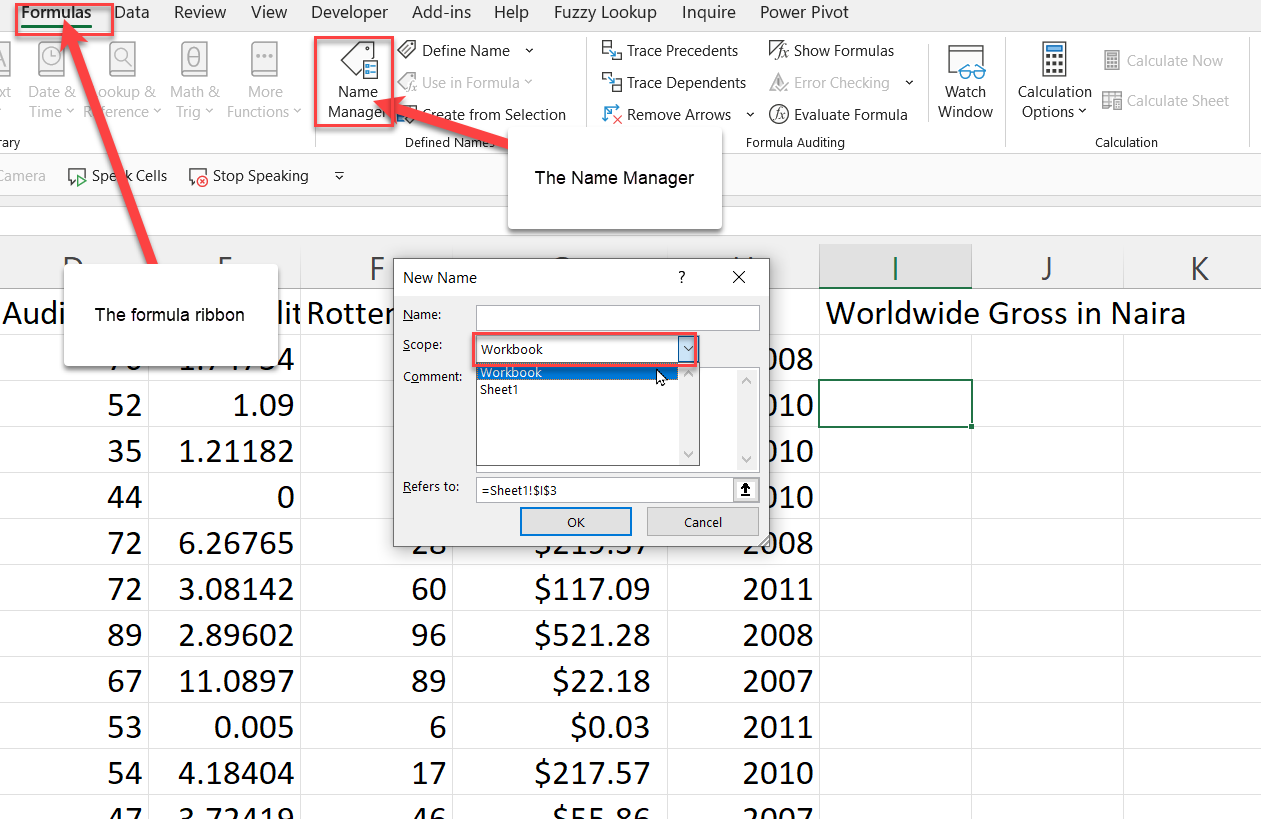
7. Define the name manger parameters:
- The name is simply what you want to call this function. I am going with NairaConvert.
- The scope should be workbook because you want to use this function in the workbook.
- The comments explains what your function does. It is acts as a documentation.
- In the refer to, you should paste the copied function syntax.
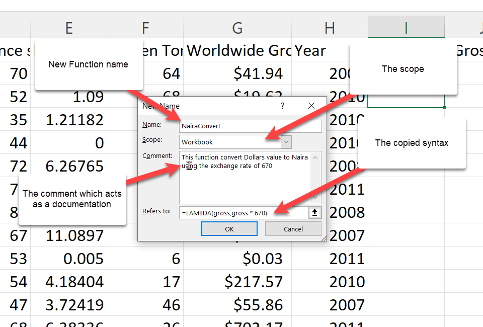
8. Press Ok.
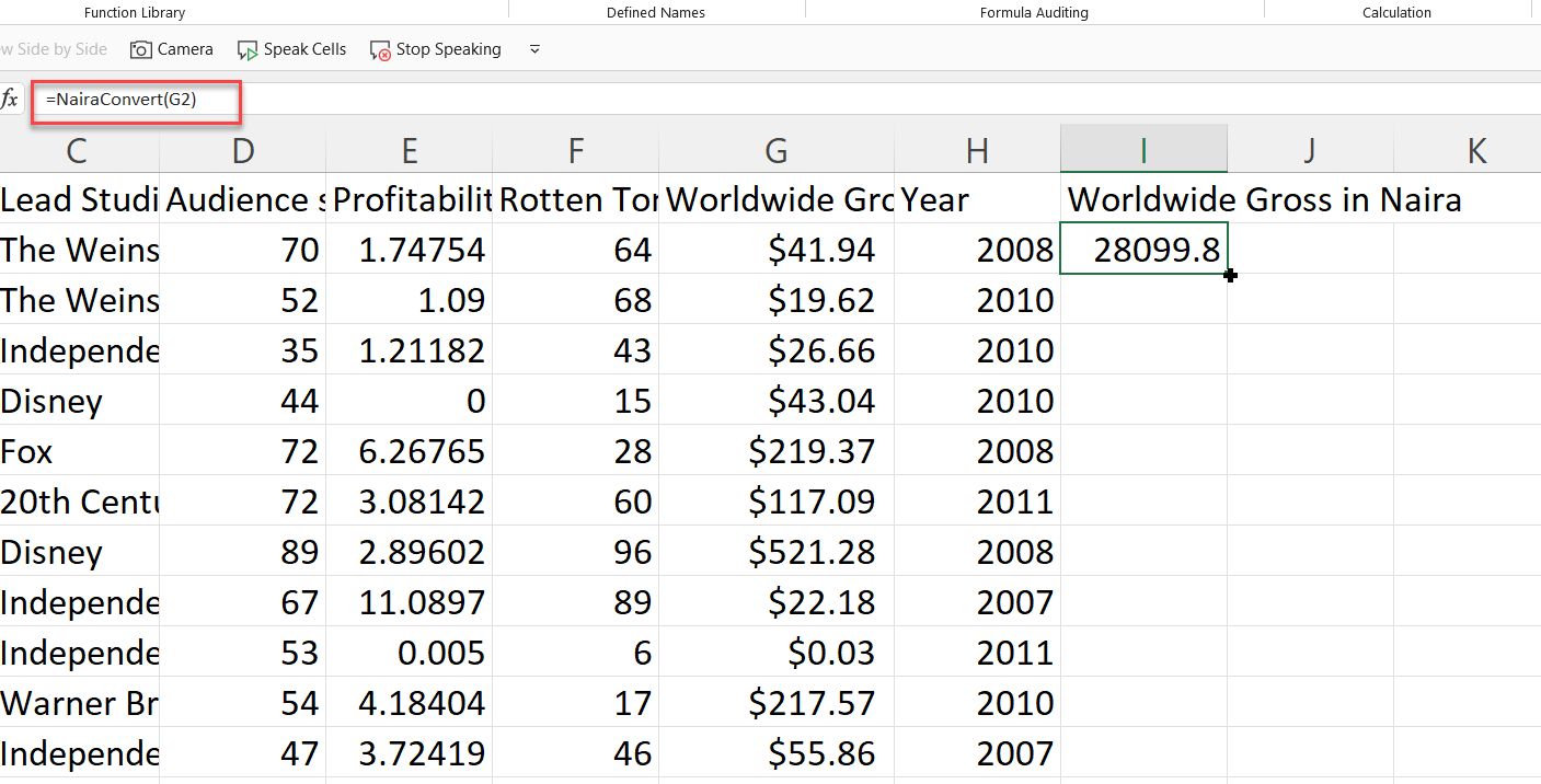
9. To use this new function, you call it with the name you defined it as—NairaConvert—and give it the gross which is our worldwise gross on G2.
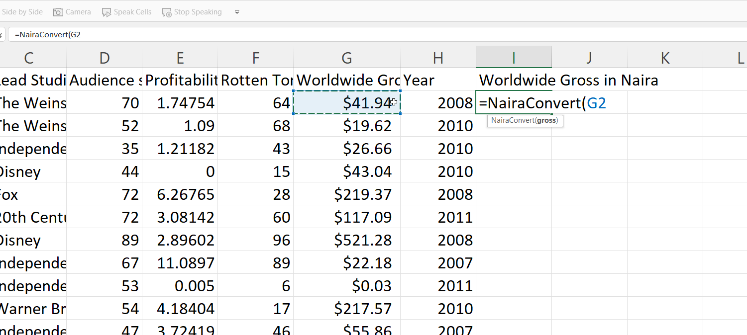
10. Close the parenthesis and press Ok
Where Can I Learn More about Excel?
There are a ton of resources for learning Microsoft Excel nowadays. So many that it is hard to figure out which ones are up-to-date and helpful.
The best thing you can do is find a helpful tutorial and follow it to completion, instead of attempting to take several at once. I would advise you to start with freeCodeCamp’s Microsoft Excel Tutorial for Beginners — Full Course, which is available on YouTube.
You should also join communities like the Microsoft Excel and Data Analysis Learning Community. However, if you’re looking for a compilation of resources, check out freeCodeCamp’s publication Excel tags.
If you enjoyed reading this article and/or have any questions and want to connect, you can find me on LinkedIn or Twitter.
Learn to code for free. freeCodeCamp’s open source curriculum has helped more than 40,000 people get jobs as developers. Get started
Being able to create a formula in Excel is fundamental to being able to use Excel well.
Writing an Excel formula is much the same as writing an equation.
With just a little bit of instruction you will be creating Excel formulas in no time! You definitely need this skill in your toolbox if you need to calculate GST or multiply and subtract using Excel formulas.
And of course, you will be able to confidently read other people’s Excel formulas which is awesome when you want to work out what the formula is actually doing.
In this blog I cover:
- Data types that can be used to create a formula in Excel
- How to create a formula in Excel using cell references
- How to write a formula in Excel
- How to create a formula in Excel for multiple cells
- How to create a formula in Excel example with download file
- How to create a formula in Excel step-by-step
Data types that can be used to create a formula in Excel
Before you start your first formula understand that only some types of data can be used in a formula.
Excel is constantly checking if a number, a date or text has been entered into a cell.
Excel formulas can only be performed using cells that contain numbers or dates. These type of cells are commonly referred to as values.
Checking the alignment of a cell’s content is a good way to check if a cell can be used in a formula.
When you enter text into a cell, Excel will automatically align the text to the left of the cell, as shown in column A in the example below. These data types cannot be used in a formula.
When a number or a date (a value) is entered into a cell the alignment will automatically be aligned to the right, as shown in column C. This data can be used in a formula.
Data that is a mixture of alpha and numbers is treated as text, as shown in column B. Alphnumeric data cannot be used in a formula.
How to create a formula in Excel using cell references
Writing Excel formulas is much the same as writing an equation. However, in Excel we begin a formula with the equals sign.
A formula can include numbers and cell references.
For example: =840*10% or =C4*D4
The formula example below shows the figures 840 and 10% will be entered in separate cells.
The result of a formula is stored in a separate cell, Cell E4.
840 has been entered in Cell C4 and 10% has been entered in Cell D4. The formula can be written as =840*10% or =C4*D4.
Both of these calculations would produce a result of 84. However, using real numbers rather than cell references can be dangerous.
If Cell C4 updates from 840 to 940, the calculation using real numbers will not update to 94 unless you re-enter the formula as =940*10%.
Choosing to write a formula using cell references rather than actual numbers is far more practical.
Any number entered in cell C4 automatically is part of the calculation. Therefore, if the calculation is written using cell references instead of real numbers, updating Cell E4 to 940 will automatically update the result to 94.
Note: when entering cell references, the column number precedes the row number in the cell address. Column references can be entered in upper or lowercase.
How to write a formula in Excel
Formulas start with an equals sign (=) and can be made up of values, cell references, mathematical operators and Excel functions. Formulas are entered manually into a cell.
To start entering a basic Excel formula:
1. Click the cell that will hold the calculation result. In our example above this would be cell E4.
2. Press the equals key (=). In our example above this would be =C4*D4. Note, all formulas must start with an equals (=) sign. This indicates to Excel that you are creating a formula. Without the equals sign the formula is seen as normal data and is entered into the cell as such.
3. Press ENTER to perform the calculation.
Excel will now display the calculated result on the worksheet, and the formula used to find the result is displayed in the Formula Bar.
This method is most useful when you are using just one standard mathematical operators such as plus, minus, multiplication and divide.
The Table below shows the standard operators that are used in Excel calculations and where to find them on your keyboard.
Tip: most of the operators can also be found on the numeric pad on your keyboard.
How to create a formula in Excel for multiple cells
Take a look at the Table above again. If you look at the first letter of each of the operator names you will notice it creates the acronym BEDMAS.
You need to be aware that Excel calculates all formulas according to the BEDMAS (also known as BODMAS, PODMAS, and PEDMAS) hierarchical structure — the order in which to calculate mathematical expressions.
When Excel calculates a formula it checks from the top to the bottom of this list and performs the calculations according to where they are placed in the hierarchy.
So when you start to create formulas that have more than one operator, the BEDMAS rule kicks in.
For example: If you wanted to calculate 7 plus (+) 3 multiplied (*) by 10 you would presume you would end up with 100, however the following happens:
Your formula would look like this = 7+3*10 result 37
37 is not the answer you would have expected.
Excel calculated the formula according to the built-in hierarchical structure where multiplication is performed before addition. Therefore Excel multiplied 3 by 10 first, and then added the 7.
To overcome this problem you would need to enter the formula as follows:
Your formula would look like this = (7+3)*10 result 100
You have now instructed Excel to calculate the addition of 7 plus 3 first by placing brackets around the calculation.
Excel now calculates this part of the equation first as bracketed formulas will always be the first calculations performed, as per the hierarchical structure.
Super tip: always use brackets when creating formula with multiple operators.
How to create a formula in Excel example with download file
Check out my video below on how to subtract the right way. Click here to download the exercise file to follow along with me and try out creating formulas to subtract, add and multiply.
For a deeper dive into creating formulas in Excel you can check out the full blog here How to subtract in Excel (minus formula).
How to create a formula in Excel step-by-step
In the following example we will create a basic Excel formula to calculate the contents of cell C4 multiplied by D4.
1. Click the cell that will hold the formula result, in this case E4 and then press the = key.
2.
Select cell C4. You can do this either by clicking the cell, using your arrow keys to move the the cell or by typing the cell reference directly into the calculation. You will notice “marching ants” around cell C4 indicating that you have selected it.
3.
Press the multiplication key on the keyboard (*).
4.
Click cell D4. The “marching ants” will highlight D4.
5. Press ENTER. The calculation result will be shown in the cell while the formula used to create the result will be displayed in the Formula Bar.
If the numbers are updated in C4 or D4, the formula in E4 will automatically display the updated result.
Was this post helpful? Let us know in the Comments below.
If you enjoyed this post check out the related posts below.
Elevate your Excel game and become a pro with our exclusive Insider Group.
Be the first to know about new tutorials, videos, and tips for Microsoft 365 products. Join us now and claim your exclusive bonus today!

How to Create a Simple Formula in Excel
To create a formula in excel must start with the equal sign “=”. If there is no equals sign, then whatever is typed in the cell will not be regarded as a formula.
Here’s how to create a simple formula, which is a formula for addition, subtraction, multiplication, and division. An addition formula using the plus sign “+”, subtraction formula using the negative sign “-“, a multiplication formula using an asterisk sign “*” and division formula using the slash “/”.
Addition Formula
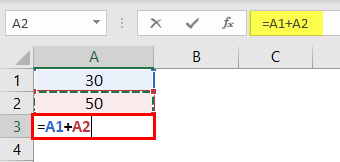
There are two numbers in cell B1 and B2. How to create a formula in excel to add both of them?

There are several ways of writing a formula. The first way is using the keyboard and the arrow keys, the second way using the keyboard and mouse and a third way to use the keyboard by typing directly the formula and the address of cell involved.
For the above addition, the formula will be used the first way.
- Place the cursor in cell B4 and then type the equals sign “=”

- Press the up arrow button, point to cell B1, the cursor turns into dashed line.

- Type the plus sign “+” for the addition operation

- Press the up arrow button again, point to cell B2

- Press the ENTER key
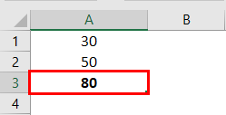
The result is as shown below

Subtraction Formula
How to write a formula in excel for subtracting number1 by number2?. The reduction formula to use the second way, i.e. using the keyboard and mouse.
- Place the cursor in cell B5 and then type the equals sign “=”
- Click cell B1 using the mouse
- Type the negative sign “-” for the subtraction operation
- Click cell B2 using the mouse
- Press the ENTER key
For more details, you can see the animation below.
Multiplication Formula
How to make a formula in excel to multiply number1 by number2. For the multiplication formula using the third way of using the keyboard by writing directly the formula and the address of the cell involved.
- Place the cursor in cell B6 and then type the equals sign “=”
- Type B1
- Type an asterisk “*” for multiplication operations
- Type B2
- Press the ENTER key
For more details, you can see the animation below.
Division Formula
How to do formulas in excel to divide number1 with number2.
- Place the cursor in cell B7 and then type the equals sign “=”
- Point the cursor to cell B1
- Type a slash mark “/” for the division operation
- Point the cursor to cell B2
- Press the ENTER key
The result is as shown below

How to View Formulas in Excel
The easiest way to see the formula in a cell is to look at the formula bar. Point the cursor to a cell that contains a formula, then the formula bar will display the formula in the cell. The location of the formula bar is below the ribbon menu.

The picture above shows the formula contained in cell B4. To see formulas in other cells just move the cursor to the desired cell and see the formula in the formula bar.
Formula bar can only display formulas in the active cell, meaning only one formula can be shown. To be able to display all the formulas in a worksheet, please read the article below “How to Display Cell Formulas in Excel”
How to Edit Formula in Excel
There are two ways to edit a formula, using the F2 key or using a formula bar.
Editing with the F2 key
Place the cursor in the cell containing the formula, then press the F2 key. The contents of the formula will appear, and the cells involved in the formula will be marked with a colored box.
The picture below shows the existing addition formula in cell B4. There are two cells involved in the formula: cell B1 and B2. The address of the cell B1 light blue colored then the cell B1 will be surrounded with the same colored line, likewise with cell B2, the color of lines around it is same as cell B2 address color.

For example, the formula will be edited by adding the number 2. Type the plus sign “+”, number 2 and then press the ENTER key.
The results are as shown below. The formula in cell B4 has changed.

Editing with the formula bar
Place the cursor in the cell containing the formula, then click on the formula bar section. The formula in the cell will appear automatically. The display will be the same as when pressing the F2 key.
The picture below shows the existing subtraction formula in cell B5. For example, the formula will be edited by subtracting the number 2. Type a negative sign “-” number 2, then press the ENTER key.
How to Copy Formula in Excel
The cell that contains the formula can be copied like any other data. The difference, which is copied is the formula, not the value of the cell and the cell address forming the formula will be changed according to the location.
See image below. Cell B4 contains a formula that adds the value of cell B1 and B2. The formula will be copied and placed in the range C4: F4.

Place the cursor in cell B4. Do a copy (CTRL + C). Select C4: F4 range, then paste it (CTRL + V).
The result is as shown below.

The value of cell C4 to F4 is not equal to the value of cell B4, because excel copied the formula, not the cell value. Cell C4 contains a formula that adds C1 and C2 values, as well as cell D4 until F4; all contain a formula that adds cell values in row 1 and row 2 in the same column.
Another way to copy formula in excel
In addition to using the keyboard, there is another way to copy the formula, which is using the mouse. Eg formula in cell B5 will be copied. Click cell B5, point mouse to bottom right of cell B5 until the cursor change shape become thinner. Click and hold, then drag the cursor until cell F5. The result is as shown below.
Is there any other way to copy the formula with the mouse, of course 😊. For example, the formula in range B6: B7 will be copied. Select range B6: B7, then right click select copy. Select range C6: F7, right click, select Paste. The result as shown below.
How to Paste Special in Excel
If the cell that contains the formula is copied, the formulas are copied, not its value. The question is what if you want to copy the value, not the formulas. The solution is using Paste Special.
For example, there are data like the image above. Range A4:F7 mostly contains the formula, what if the range is copied and placed on the range A9:F11?.
Select range A4:F7. Do a copy (CTRL+C). Place the cursor in cell A9, and then do a paste (CTRL + V). The results are as shown below.

The results are different. If checked, cell B9 contains formula =B6+B7, as well as other cells in range B9:F12, all containing formulas.
For copying its value only. Select range A4:F7. Do a copy (CTRL+C). Place the cursor in cell A9, and then do a paste special (CTRL+ALT+V). A dialog box appears as shown below. Select “Values”, then click OK.

The results are shown below.

The results are equal to the range A4: F7. If rechecked, the content of cell B9 and other cells in the range B9:F12 is not a formula but a number.
How to Display Cell Formulas in Excel
To see the existing formula in a cell already discussed earlier. There is one drawback, only can see the formula in one cell only. If you want to see all the formulas that exist in the worksheet, the only way is to use the “Show Formulas” command.
The location is on Ribbon Menu, Formulas tab, auditing group formula. Click once, then all data generated from formula will show its formula. Click once again; it will return to its original state.
If you want to use the Show Formulas command faster, use the shortcut CTRL + ` (grave accent, in the left position of keyboard 1 and above the left tab)
Excel Write Formula (Table of Contents)
- Writing Formula in Excel
- How to Write Formula in Excel?
Writing Formula in Excel
What would be your answer when I ask you, “What is Excel?” A tool that helps to store, slicing and dicing the data plus a tool that can help us calculate sums, percentages, interest rates, etc., right? The most essential as well as an important part of Excel is a formula. The formula is nothing but an equation that allows you to perform various calculations under Microsoft Excel. These formulae are the easiest way of calculation based on the given data. However, being new to Excel, you might not always be able to handle the Excel formulae. It is very easy and simple, though, to add formulae under Excel. This article will try to make you literate about how to write different formulae under Excel, and you will be master in applying the same after going through this article.
Let’s see how we can create/write a formula under Excel.
The first thing we should know is, every Excel formula starts with the equals to sign (‘=’) inside an Excel cell. After this sign, you can write the equation in which you want Excel to perform calculations or any inbuilt function name (Ex. SUM), which performs a calculation and returns the output in a given cell.
How to Write Formula in Excel?
Let’s understand How to Write the formula in excel with a few examples.
You can download this Write Formula Excel Template here – Write Formula Excel Template
Example #1
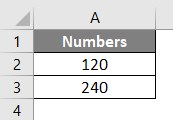
Step 1: Suppose we have two numbers, 120 and 240, in cell A1 and A2, respectively, in the Excel sheet. See the screenshot below:
Now, I want to add these two numbers; We’ll see how this can be achieved.
Step 2: In cell A4, start typing the equation by simply using equals to sign and then use 120 + 240 to add these two values up. See the screenshot below for a better understanding.
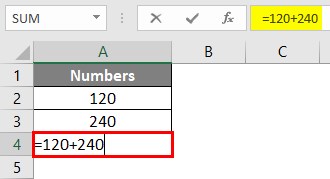
Step 3: Press Enter Key to see the result. You can see 360 as a result of cell A4, as shown below.
This is how a basic formula can be entered under Microsoft Excel. Now, what if we change the numbers in cell A1 and A2 to some different values? Will the formula under cell A3 change values? Well, let’s see by doing so.
Step 4: Change the numbers in cell A1 and A2 to 120 and 240, respectively.
If you will check cell A3, it is still showing the result for old values (i.e. 120 + 140 = 360). Because in cell A3, we have used the equation as 120 + 140. These are values that are fixed and not dynamic ones. Therefore, in order to get rid of such a situation, Excel also provides an option to be able to use dynamic ranges under an equation/formula for that sake.
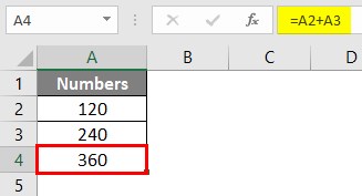
Step 5: In cell A3, tweak the formula to =A2+ A3. What we tried doing here is, instead of giving a number as an argument, we have supplied the cells which contain a number as an argument. This will be beneficial when you change the numbers in cells A2, A3; values in cell A4 will automatically change after performing the operations. This is how making you formula dynamic using a range of cells work.
After using the above formula, the output is shown below:
Now, if I change the values under cell A1 and A2, the results in cell A3 will automatically change. See the screenshot below.
Example #2
Excel has a more user-friendly approach when it comes to applying the formula. You just can simply copy-paste the formula from one cell to another by dragging it through. Let’s see how to do it.
Suppose we have data as shown below across the first and second row of different columns (A to E), and we wanted to get a sum for each column in their third row, respectively. We’ll see how excel works in this situation.
Step 1: In cell A3, create an equation using a dynamic range of cells that sums the values under A1 and A2. You can use =A1+A2 as a formula under cell A3 to get the sum of the numbers within those cells.
Also, Press Enter key to see the output in cell A3.
Step 2: Now, select the cell A3 and then drag the formula across A3 to E3 to apply the same formula that sums up the first and second row for each column. You should get the output as shown in the screenshot below:
Well, you have multiple ways to achieve this result. You can select the entire third row across column A to E and just press Ctrl + R to copy and paste the formula under cell A3 to other columns. Or else, you can copy the formula under cell A3 by Ctrl + C and paste it one by one in each of B3, C3, D3, E3 to achieve the same result.
Example #3
In this example, we will work on using the built-in Excel functions. How to use the built-in Excel function to perform a task (ex. Summing number across the rows).
Consider the same data as shown in example 2, and we wanted to have sum of the first two rows of each column within the third row. However, this time we will use a built-in Excel function named SUM to achieve this result.
Step 1: In cell A3, start typing =SUM; it will pop up a list of all functions that contain SUM as a keyword. Select the SUM function through that list by double-clicking on it.
Step 2: Select the range of cells A1 to A2 with the use of your computer mouse or laptop touchpad as an argument to the SUM function. Because these are the cells that we wanted to sum up.
Well, you also can use the comma to separate the values instead of these ranges.
Step 3: Complete this formula by adding closing parentheses at the end of this function and press the Enter key to get the sum of cell A1 and A2 under cell A3.
This function precedes the equation we use in Example 2 by a huge margin when we have tons of data. Ex. Consider you have 5 Lacs Excel Rows, and you wanted to sum those up. You surely would not like to input each cell reference for 5 Lacs of time, would you?
Step 4: You can drag this formula across the different columns for the same row or user Ctrl + R to populate it across all the rows or copy and paste one by one to each column. The choice is all yours. You’ll get the final output as shown below:
This is it from this article. Let’s wrap the things up with some points to be remembered:
Things to Remember About Write Formula in Excel
- In order to be able to use a formula in Excel, you need to start it with equals to sign. You also can start a formula with a Plus or minus sign.
- You can have different operational formulae of your own for subtraction, multiplication, division, squaring a number, etc. However, all these operations are better to do with built-in Excel functions because these functions precede over operational formulae.
Recommended Articles
This is a guide to Write Formula in Excel. Here we discuss How to use Write Formula in Excel along with practical examples and a downloadable excel template. You can also go through our other suggested articles –
- Excel DEGREES Function
- Compare Two Lists in Excel
- Excel Text with Formula
- TIME in Excel
Вычисление по формулам – пожалуй, самая полезная функция программы Excel. Она не только экономит время пользователя, но и исключает возможность арифметических ошибок, допускаемых человеком. Конечно, эти плюсы достижимы только тогда, когда формулы созданы и работают правильно. Как и в любом деле, учиться грамотно составлять формулы в Эксель нужно с простейших и планомерно двигаться к более сложным вычислениям.
В этом уроке мы предоставим расширенное практическое руководство по тому, как правильно создавать формулы в Microsoft Excel.
Содержание
- Составление элементарных формул
- Оператор формул в Excel
- Примеры вычислений
- Создание формул со скобками
- Использование Excel в качестве калькулятора
- Заключение
Составление элементарных формул
Проще всего в Эксель создаются формулы из четырех арифметических действий — сложения, вычитания, умножения и деления. При этом данные для вычислений должны находиться в разных ячейках/столбцах/строках.
- Для начала нужно выбрать свободную ячейку и напечатать в ней знак “=”. Для программы это будет сигналом, что в этой ячейке будет производиться расчет по формуле.

Другой способ перевести ячейку в режим формулы — щелкнуть по ней левой кнопкой мыши, а знак равенства напечатать в строке формул.

Эти 2 способа выше дублируют друг друга и можно выбрать тот, который больше по душе.
- Далее начинаем писать формулу. Допустим, мы хотим просуммировать ячейки B2-B7. Тогда в ячейке B8 (можно выбрать любую другу свободную ячейку) после знака “=” щелкаем курсором по B2 (ее контур начинает пульсировать, а координата ячейки появляется в формуле), далее ставим знак “+”, выделяем следующую ячейку, далее снова знак “+” и так далее. В конечном виде формула выглядит так: =B2+B3+B4+B5+B6+B7

- Как только мы перечислим все ячейки, нажимаем клавишу “ENTER”, чтобы получить результат.


Оператор формул в Excel
Вместо знака “+” в формуле можно использовать знаки вычитания, умножения и деления, при этом в Эксель есть специальные знаки для этих математических действий, которые называются операторами формул:
- Плюс – это знак “+”
- Минус – это знак “-” (дефис).
- Умножение – это знак “*” (звездочка).
- Деление – это знак “/” (слэш или косая черта).
- Возведение в степень – это знак “^” (циркумфлекс, находится на клавише с цифрой 6, печатается вместе с зажатой клавишей Shift).
А так могут выглядеть формулы в ячейке:
- =А1-А2
- =А1/А2
- =А1*А2
Примечание: все знаки должны идти без пробелов.
Также, в формулах может быть задействовано сколько угодно ячеек из различных строк и столбцов (=А1+А2+А3+А4+В6… и т.д), а результирующей может быть любая свободная ячейка.
Примеры вычислений
Попробуем применить полученные знания на деле. Например, у нас есть заполненная таблица. В первом столбце указано наименование товара (разновидности велосипедов), во втором столбце – количество проданных штук, в третьем — цена за 1 штуку. Мы можем посчитать, на какую общую сумму был продан каждый вид велосипеда. Сделаем это, умножив цену за 1 штуку на количество проданных штук.

- В ячейке D2, которая станет результирующей, ставим знак “=”, далее выделяем ячейку B2, ставим знак “*” и выделяем ячейку C2. Так формула выглядит в конечном виде: =B2*C2

- Формула готова. Жмем “ENTER” и получаем результат умножения.

- Теперь то же самое действие можно выполнить для остальных наименований в других строках. Причем, создавать каждый раз одинаковую формулу вовсе не обязательно, более того, это будет лишней тратой времени.В Excel на этот случай есть отличный способ. Щелкаем на результирующей ячейке. Ее контур в правом нижнем углу имеет форму небольшого квадрата. Зажав этот квадрат левой кнопкой мыши, тянем курсор, который принял вид плюса, вниз до последней строки, в которой хотим произвести аналогичный расчет.
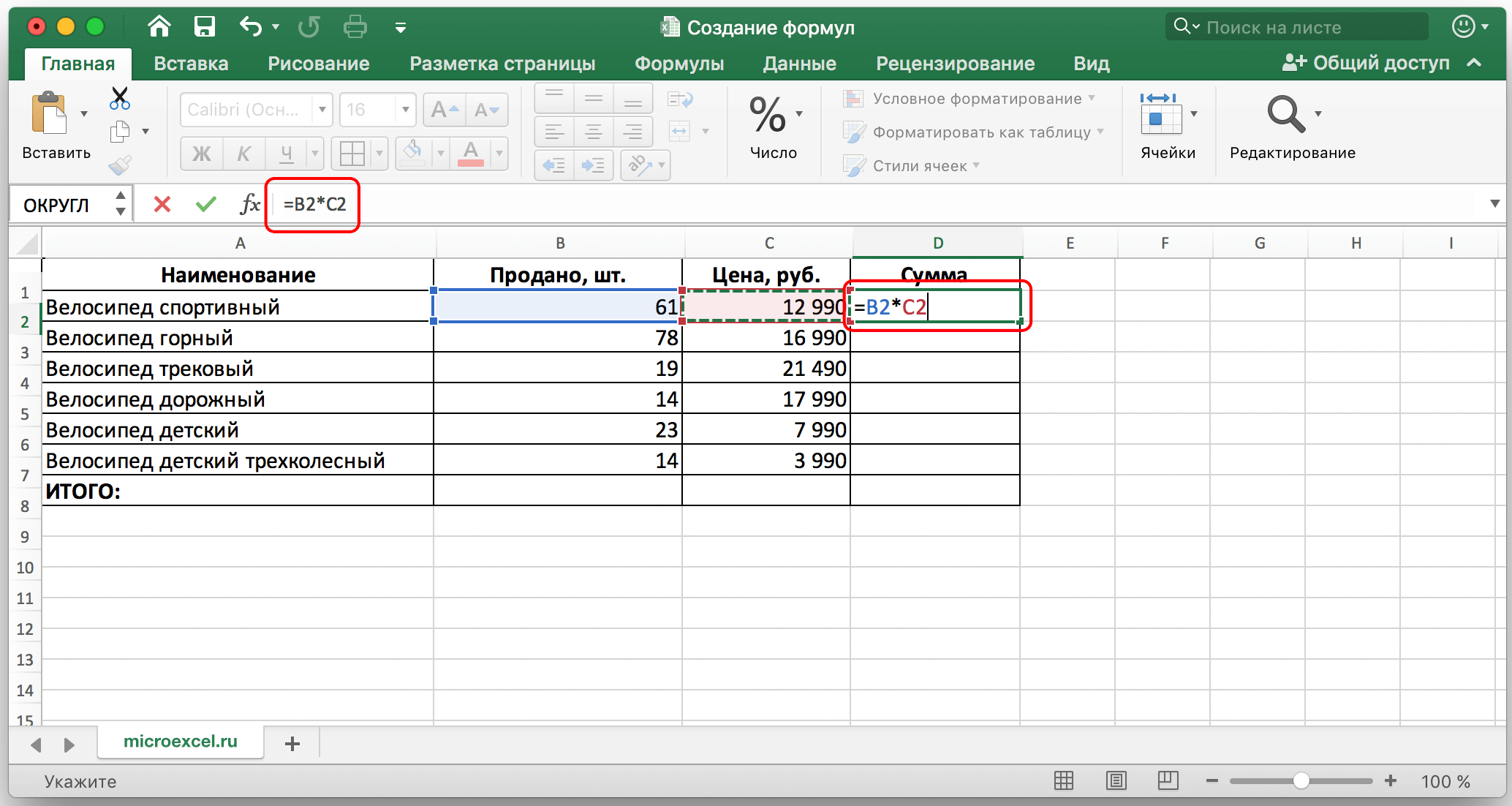


Таким образом, формула будет продублирована во всех ячейках, через которые протянули курсор, причем в каждой строке программа, скопировав начальный вариант формулы, автоматически изменит координаты строк, заменив их на необходимые, чтобы расчет были правильными.

Создание формул со скобками
Excel – мощный инструмент для работы с таблицами и выполнения сложнейших расчетов, потому в нем легко можно работать с большим количество данных, а формулы нужно составлять, руководствуясь законами математики.
Допустим, у нас есть данные по продажам за 1 и 2 квартала, при этом цена товара оставалась неизменной. Узнать нужно общую сумму реализованного товара за 1-2 кварталы.

Для начала нужно сложить количество проданного товара в 1 и 2 кварталах, и далее умножить полученную сумму на цену за 1 штуку.
Произвести расчет можно сразу по одной формуле. По правилам математики, действие сложения нужно брать в скобки, иначе первым выполнится умножение (что даст неверный результат). В Excel действуют те же самые правила, и используются классические знаки скобок (открывающих и закрывающих).
- Ставим курсор на результирующую ячейку (E2), пишем знак “=”, далее открываем скобку, в ней складываем ячейки B2 и C2, далее скобку закрываем, ставим знак умножения и, наконец, координаты ячейки D2. Так формула выглядит в конечном виде: =(B2+C2)*D2

- Формула готова. Теперь жмем клавишу “ENTER”, чтобы увидеть результат вычислений.

- При желании и необходимости, формулу можно протянуть на остальные строки, как это было описано выше.


Примечание: Стоит отметить, что вовсе не обязательно все ячейки, участвующие в формуле, располагать по соседству или на одном листе Excel. Пусть даже они будут на разных листах — результат получится правильный, если формула составлена корректно.
Использование Excel в качестве калькулятора
Программу Excel можно использовать как обычный калькулятор. Ставим знак “=” в любой ячейке, пишем нужную формулу, а затем нажимаем ” ENTER”, чтобы получить результат.

Заключение
Таким образом, программа Microsoft Excel дает пользователю широкие возможности при работе с числами, а простейшие арифметические действия (сложение, вычитание, умножение, деление) выполняются достаточно легко и требует лишь знаний самих законов математики, не более того.