
Excel for Microsoft 365 Excel for Microsoft 365 for Mac Excel 2021 for Mac Excel 2019 Excel 2019 for Mac Excel 2016 Excel 2016 for Mac Excel 2013 Excel 2010 More…Less
If you have tasks in Microsoft Excel that you do repeatedly, you can record a macro to automate those tasks. A macro is an action or a set of actions that you can run as many times as you want. When you create a macro, you are recording your mouse clicks and keystrokes. After you create a macro, you can edit it to make minor changes to the way it works.
Suppose that every month, you create a report for your accounting manager. You want to format the names of the customers with overdue accounts in red, and also apply bold formatting. You can create and then run a macro that quickly applies these formatting changes to the cells you select.
How?
|
|
Before you record a macro Macros and VBA tools can be found on the Developer tab, which is hidden by default, so the first step is to enable it. For more information, see Show the Developer tab. |


|
|
Record a macro
|

|
|
Take a closer look at the macro You can learn a little about the Visual Basic programming language by editing a macro. To edit a macro, in the Code group on the Developer tab, click Macros, select the name of the macro, and click Edit. This starts the Visual Basic Editor. See how the actions that you recorded appear as code. Some of the code will probably be clear to you, and some of it may be a little mysterious. Experiment with the code, close the Visual Basic Editor, and run your macro again. This time, see if anything different happens! |

Next steps
-
To learn more about creating macros, see Create or delete a macro.
-
To learn about how to run a macro, see Run a macro.
How?
|
|
Before you record a macro Make sure the Developer tab is visible on the ribbon. By default, the Developer tab is not visible, so do the following:
|
|
|
Record a macro
|
|
|
Take a closer look at the macro You can learn a little about the Visual Basic programming language by editing a macro. To edit a macro, in the Developer tab, click Macros, select the name of the macro, and click Edit. This starts the Visual Basic Editor. See how the actions that you recorded appear as code. Some of the code will probably be clear to you, and some of it may be a little mysterious. Experiment with the code, close the Visual Basic Editor, and run your macro again. This time, see if anything different happens! |
Need more help?
You can always ask an expert in the Excel Tech Community or get support in the Answers community.
Need more help?
Want more options?
Explore subscription benefits, browse training courses, learn how to secure your device, and more.
Communities help you ask and answer questions, give feedback, and hear from experts with rich knowledge.
How to Create Macros in Excel: Step-by-Step Tutorial (2023)
Get ready to have your mind blown! 🤯
Because in this tutorial, you learn how to create your own macros in Excel!
That’s right! And you don’t need to know VBA (Visual Basic for Applications)!
Instead, you will use the Excel macro recording feature to send your spreadsheet experience into overdrive! 🚀
So, read on and try it out yourself using this practice Excel workbook.
What are Excel macros?
A macro is a small program or set of actions that you can run repeatedly. Excel macros are used to automate repetitive tasks to save a lot of time and hassle.
For example, open and take a look at the practice Excel workbook.

Businesses would often have lists like this one. These are potential customers they might want to reach out to and market their products.
Notice how Columns C to H are just pieces of information extracted from Columns A & B.
(Learn how to extract strings from texts in this tutorial!)
To streamline the worksheet, you can hide Columns A & B. You can also hide the rest of the columns on the right starting from Column I.
Let’s do this using Excel macros!
How to record Excel macros
1. Click on the View tab in the Excel ribbon

2. Next, click on the Macros button on the right side of the View ribbon

3. This will open the Macros drop-down.
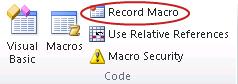
Click Record Macro.

4. Enter a name for your macro, something like Hide_Columns.

Excel macros can be stored in the Personal Macro Workbook. This is saved in the system files of Microsoft Excel and macros saved here can be used in other workbooks.
For this Excel macro tutorial, you only need to save the macros in the current Excel file.

4. Select Store macro in: This Workbook then click the OK button.
Excel is now recording your actions to create a macro.
5. Select Columns A & B and then right-click on the highlighted Column Bar to Hide them.

6. Then select Column I and press Ctrl + Shift + Right Arrow to include all remaining columns on the right.
7. Right-click on the highlighted Column Bar then click on Hide.
Your worksheet should now look like this:

To end the macro recording:
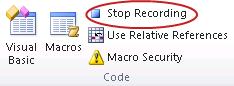
8. On the View ribbon, click on Macros and select Stop Recording.

Good job! 👏
You have created your first macro in Excel!
But wait, where is the recorded macro?
To view all of the available Excel macros :
1. Select View Macros.

2. This opens the Macro window. Saved macros will be listed here and you can Run whichever one you need.
You can also click on Edit to view the VBA code window.

3. The VBA code editor opens.

Notice the Hide_Columns Sub procedure. You don’t have to write or edit VBA code for the macro.
Excel automatically generated each code line based on the recorded keystrokes and mouse clicks.
The Record Macro feature is powerful enough for general spreadsheet automation needs.
But if you want to customize your own VBA macro, you can learn more about Visual Basic for Applications (VBA) here.
Using the Developer tab
Let’s record another macro to Unhide the hidden columns.
This time, you can record the macro from the Developer tab.
The Developer tab gives you access to a lot of useful Microsoft Excel features such as the Visual Basic Editor. It also allows you to quickly insert form controls such as buttons and checkboxes.
However, the Developer tab is not visible in the Excel ribbon by default.
To add it:
1. Right-click on the Excel ribbon.
Select Customize the Ribbon.

2. This opens the Customize Ribbon window.
On the right side, check the Developer tab checkbox.

3. You should now see the Developer tab.

To start recording the Unhide macro:
1. Click on the Record Macro button in the Developer tab.

2. Name this macro Unhide_Columns.

3. Click OK.
The recording has started.
4. Press Ctrl + A twice to select all cells.
5. Right-click anywhere on the Column Bar then click Unhide.

6. Click on the Stop Recording macro button to finish up.

Great work! 👌
Now you have two recorded macros that can be executed.
How to run an Excel macro
To run your macros:
1. Click on the Macros button from the Developer tab.

2. In the Macro window, select the macro Hide_Columns and click on Run.

The macro executes the actions recorded earlier and hides the unnecessary columns.
You can also run macros from the View ribbon.
Run Excel macro from the View tab
This time, run the Unhide_Columns to show all the columns.
1. On the View ribbon, click the Macros button and select View Macros.
2. Select the Unhide_Columns macro and Run it.

This unhides all the columns in the worksheet.
As you can see, the Macro window allows you to quickly run all the available macros.
But you can execute them even faster by using buttons and shortcuts ❗
Run Excel macro from a button
For this next example, you will assign macros to buttons which will be located on top of the table.
1. Insert 2 rows above the table headers. Select Row 1 then press Ctrl + Shift + Plus Sign(+) twice.

2. To create a button, click on Insert > Illustrations > Shapes.
Then select the Rectangle.

3. Draw a rectangle and format it as you’d like. Label it “HIDE”.

This will be your HIDE button. Place it between columns A & B so it will be hidden with the columns when the macro runs.
4. To assign a macro, right-click the shape and select Assign Macro.

5. In the Assign Macro window, select Hide_Columns and click OK.

The Hide button now works!
Now, do the same for the Unhide_Columns macro.
6. Create another rectangle button and label it “UNHIDE”.

7. Repeat Steps 4 & 5 but this time, assign the Unhide_Columns macro.
Alright! 👍
Now you can quickly run your macros using the HIDE and UNHIDE buttons.

Run Excel macro from a shortcut key
It is sometimes better to run macros using a keyboard shortcut.
For this next example, you want to quickly highlight people on the list that expressed interest in the business.
To create a macro for this:
1. Select any cell within the table.

2. On the Developer tab, toggle ON the Use Relative References button.

3. Start recording with the Record Macro button on the Developer tab.
Or, you can also click the Record Macro button on the Status Bar.

4. Name the macro Mark_Interested.
Then assign a shortcut key. For example, Ctrl + Q.

Click OK. The recording has now started.
4. Highlight the row of the Active Cell using the keyboard shortcut Shift + Space Bar.

When selecting cells or expanding selections while recording a macro, it is best to use keyboard shortcuts.
This is so that Excel can record the selections as relative references.
For example, if you select Row 4 by clicking on the Row Bar, Excel will record this as an absolute reference. This means it will always select Row 4 regardless of the currently Active Cell.
When you use the Shift + Space Bar shortcut instead, it tells Excel to select the row of the current Active Cell.
5. Apply the formatting:
- Fill using the color Green
- Change font color to White

6. End the macro recording from the Status Bar

All done!
Try to use the shortcut Ctrl + Q to quickly apply formatting to entire rows.

Saving macro-enabled workbooks
If you save the practice workbook, this window will pop up:

This is because the practice workbook is currently saved with the .xlsx file extension which does not support macro features.
To save properly, change it to the .xlsm file extension for macro-enable workbooks.
Keep this in mind when saving your work.
Congratulations! 🤩
You are now familiar with Excel macros.
Try to record your own macros and start saving time ⏱️ on your work!
That’s it – Now what?
The examples above are very useful though they are quite simple.
You can record macros for more complex functions. Such as creating custom charts or selectively copying rows of data to another workbook.
But recording and playing macros is just the tip of the iceberg.
With VBA programming, you get access to a whole different level of Excel automation. 🤖
And while Visual Basic may seem overwhelming at first, you can start slow with basic variables and IF statements. These are much easier than you might think!
Learn all that and much more in my free 30-minute online VBA course here.
Other resources
If you want to know more about the inner workings of the record macro feature, check out my Excel macro tutorial for beginners on YouTube.
You can also dive right into VBA by reading this article or watching this introductory video on VBA and macros!
Hope you enjoyed this article!
Kasper Langmann2023-01-19T12:25:15+00:00
Page load link
Developer Tab | Command Button | Assign a Macro | Visual Basic Editor
With Excel VBA you can automate tasks in Excel by writing so called macros. In this chapter, learn how to create a simple macro which will be executed after clicking on a command button. First, turn on the Developer tab.
Developer Tab
To turn on the Developer tab, execute the following steps.
1. Right click anywhere on the ribbon, and then click Customize the Ribbon.

2. Under Customize the Ribbon, on the right side of the dialog box, select Main tabs (if necessary).
3. Check the Developer check box.

4. Click OK.
5. You can find the Developer tab next to the View tab.

Command Button
To place a command button on your worksheet, execute the following steps.
1. On the Developer tab, click Insert.
2. In the ActiveX Controls group, click Command Button.

3. Drag a command button on your worksheet.
Assign a Macro
To assign a macro (one or more code lines) to the command button, execute the following steps.
1. Right click CommandButton1 (make sure Design Mode is selected).
2. Click View Code.

The Visual Basic Editor appears.
3. Place your cursor between Private Sub CommandButton1_Click() and End Sub.
4. Add the code line shown below.

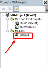
Note: the window on the left with the names Sheet1 (Sheet1) and ThisWorkbook is called the Project Explorer. If the Project Explorer is not visible, click View, Project Explorer. If the Code window for Sheet1 is not visible, click Sheet1 (Sheet1). You can ignore the Option Explicit statement for now.
5. Close the Visual Basic Editor.
6. Click the command button on the sheet (make sure Design Mode is deselected).
Result:

Congratulations. You’ve just created a macro in Excel!
Visual Basic Editor
To open the Visual Basic Editor, on the Developer tab, click Visual Basic.

The Visual Basic Editor appears.

#Руководства
- 23 май 2022
-

0
Как с помощью макросов автоматизировать рутинные задачи в Excel? Какие команды они выполняют? Как создать макрос новичку? Разбираемся на примере.
Иллюстрация: Meery Mary для Skillbox Media

Рассказывает просто о сложных вещах из мира бизнеса и управления. До редактуры — пять лет в банке и три — в оценке имущества. Разбирается в Excel, финансах и корпоративной жизни.
Макрос (или макрокоманда) в Excel — алгоритм действий в программе, который объединён в одну команду. С помощью макроса можно выполнить несколько шагов в Excel, нажав на одну кнопку в меню или на сочетание клавиш.
Обычно макросы используют для автоматизации рутинной работы — вместо того чтобы выполнять десяток повторяющихся действий, пользователь записывает одну команду и затем запускает её, когда нужно совершить эти действия снова.
Например, если нужно добавить название компании в несколько десятков документов и отформатировать его вид под корпоративный дизайн, можно делать это в каждом документе отдельно, а можно записать ход действий при создании первого документа в макрос — и затем применить его ко всем остальным. Второй вариант будет гораздо проще и быстрее.
В статье разберёмся:
- как работают макросы и как с их помощью избавиться от рутины в Excel;
- какие способы создания макросов существуют и как подготовиться к их записи;
- как записать и запустить макрос начинающим пользователям — на примере со скриншотами.
Общий принцип работы макросов такой:
- Пользователь записывает последовательность действий, которые нужно выполнить в Excel, — о том, как это сделать, поговорим ниже.
- Excel обрабатывает эти действия и создаёт для них одну общую команду. Получается макрос.
- Пользователь запускает этот макрос, когда ему нужно выполнить эту же последовательность действий ещё раз. При записи макроса можно задать комбинацию клавиш или создать новую кнопку на главной панели Excel — если нажать на них, макрос запустится автоматически.
Макросы могут выполнять любые действия, которые в них запишет пользователь. Вот некоторые команды, которые они умеют делать в Excel:
- Автоматизировать повторяющиеся процедуры.
Например, если пользователю нужно каждый месяц собирать отчёты из нескольких файлов в один, а порядок действий каждый раз один и тот же, можно записать макрос и запускать его ежемесячно.
- Объединять работу нескольких программ Microsoft Office.
Например, с помощью одного макроса можно создать таблицу в Excel, вставить и сохранить её в документе Word и затем отправить в письме по Outlook.
- Искать ячейки с данными и переносить их в другие файлы.
Этот макрос пригодится, когда нужно найти информацию в нескольких объёмных документах. Макрос самостоятельно отыщет её и принесёт в заданный файл за несколько секунд.
- Форматировать таблицы и заполнять их текстом.
Например, если нужно привести несколько таблиц к одному виду и дополнить их новыми данными, можно записать макрос при форматировании первой таблицы и потом применить его ко всем остальным.
- Создавать шаблоны для ввода данных.
Команда подойдёт, когда, например, нужно создать анкету для сбора данных от сотрудников. С помощью макроса можно сформировать такой шаблон и разослать его по корпоративной почте.
- Создавать новые функции Excel.
Если пользователю понадобятся дополнительные функции, которых ещё нет в Excel, он сможет записать их самостоятельно. Все базовые функции Excel — это тоже макросы.
Все перечисленные команды, а также любые другие команды пользователя можно комбинировать друг с другом и на их основе создавать макросы под свои потребности.
В Excel и других программах Microsoft Office макросы создаются в виде кода на языке программирования VBA (Visual Basic for Applications). Этот язык разработан в Microsoft специально для программ компании — он представляет собой упрощённую версию языка Visual Basic. Но это не значит, что для записи макроса нужно уметь кодить.
Есть два способа создания макроса в Excel:
- Написать макрос вручную.
Это способ для продвинутых пользователей. Предполагается, что они откроют окно Visual Basic в Еxcel и самостоятельно напишут последовательность действий для макроса в виде кода.
- Записать макрос с помощью кнопки меню Excel.
Способ подойдёт новичкам. В этом варианте Excel запишет программный код вместо пользователя. Нужно нажать кнопку записи и выполнить все действия, которые планируется включить в макрос, и после этого остановить запись — Excel переведёт каждое действие и выдаст алгоритм на языке VBA.
Разберёмся на примере, как создать макрос с помощью второго способа.
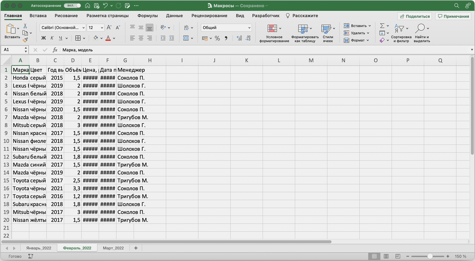
Допустим, специальный сервис автосалона выгрузил отчёт по продажам за три месяца первого квартала в формате таблиц Excel. Эти таблицы содержат всю необходимую информацию, но при этом никак не отформатированы: колонки слиплись друг с другом и не видны полностью, шапка таблицы не выделена и сливается с другими строками, часть данных не отображается.
Скриншот: Skillbox Media
Пользоваться таким отчётом неудобно — нужно сделать его наглядным. Запишем макрос при форматировании таблицы с продажами за январь и затем применим его к двум другим таблицам.
Готовимся к записи макроса
Кнопки для работы с макросами в Excel находятся во вкладке «Разработчик». Эта вкладка по умолчанию скрыта, поэтому для начала разблокируем её.
В операционной системе Windows это делается так: переходим во вкладку «Файл» и выбираем пункты «Параметры» → «Настройка ленты». В открывшемся окне в разделе «Основные вкладки» находим пункт «Разработчик», отмечаем его галочкой и нажимаем кнопку «ОК» → в основном меню Excel появляется новая вкладка «Разработчик».
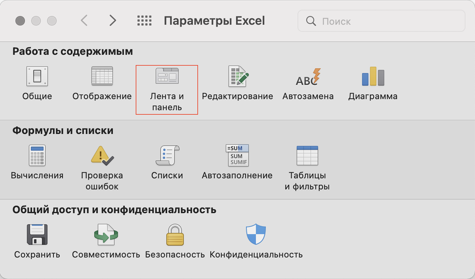
В операционной системе macOS это нужно делать по-другому. В самом верхнем меню нажимаем на вкладку «Excel» и выбираем пункт «Параметры…».
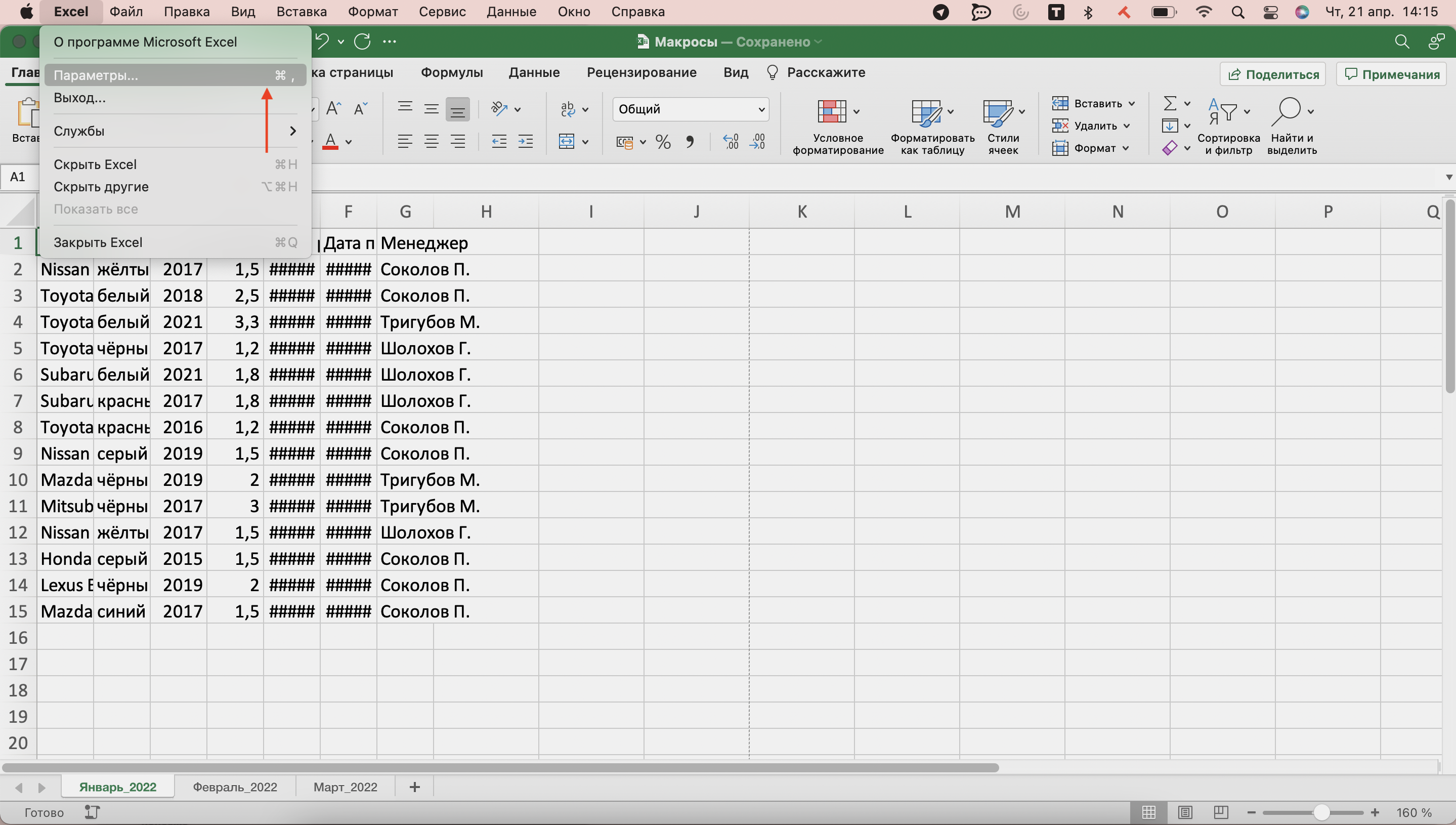
Скриншот: Skillbox Media
В появившемся окне нажимаем кнопку «Лента и панель».
Скриншот: Skillbox Media
Затем в правой панели «Настроить ленту» ищем пункт «Разработчик» и отмечаем его галочкой. Нажимаем «Сохранить».
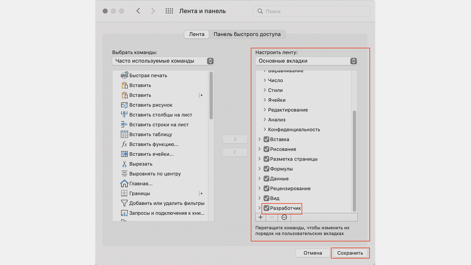
Скриншот: Skillbox Media
Готово — вкладка «Разработчик» появилась на основной панели Excel.
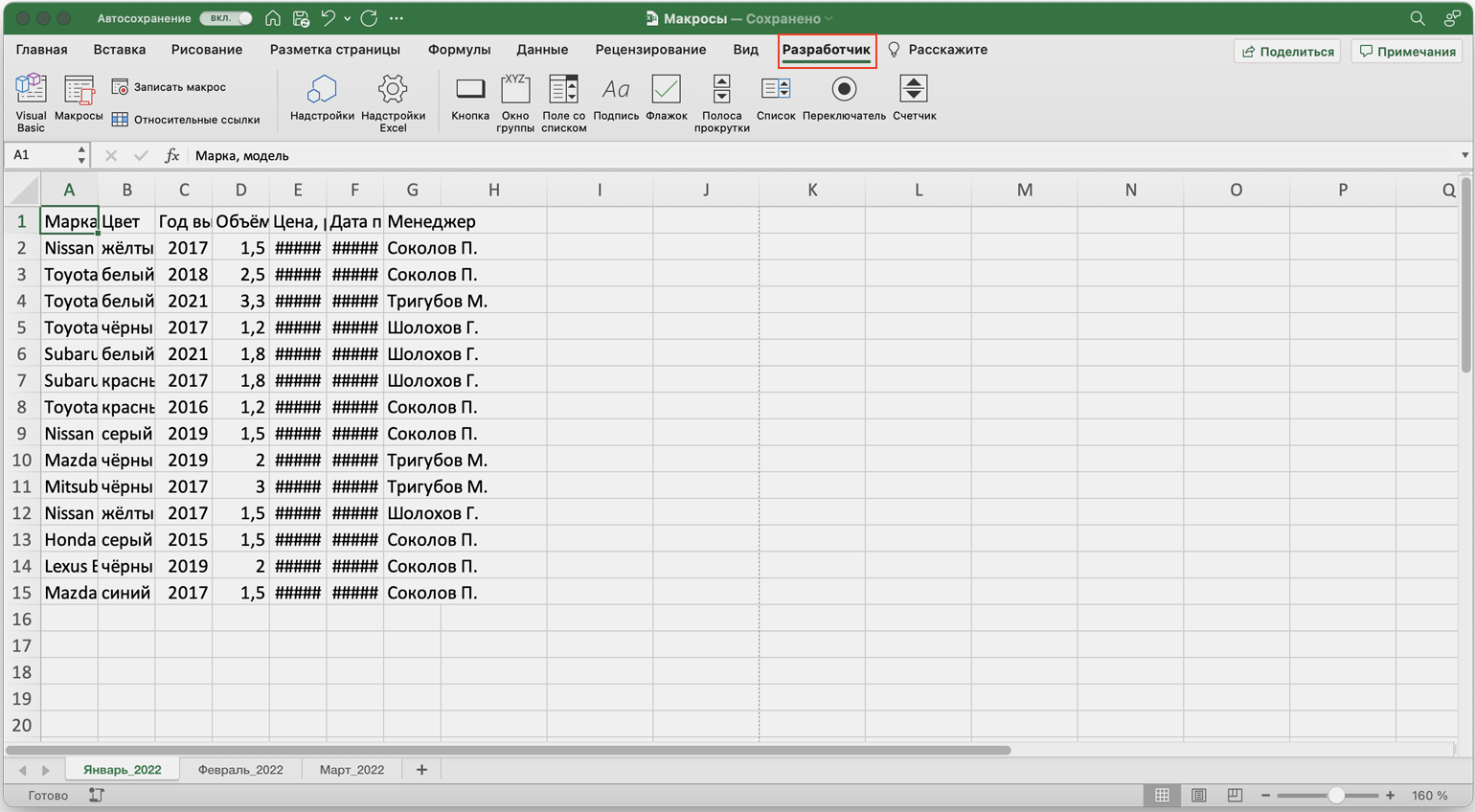
Скриншот: Skillbox Media
Чтобы Excel смог сохранить и в дальнейшем использовать макрос, нужно пересохранить документ в формате, который поддерживает макросы. Это делается через команду «Сохранить как» на главной панели. В появившемся меню нужно выбрать формат «Книга Excel с поддержкой макросов».
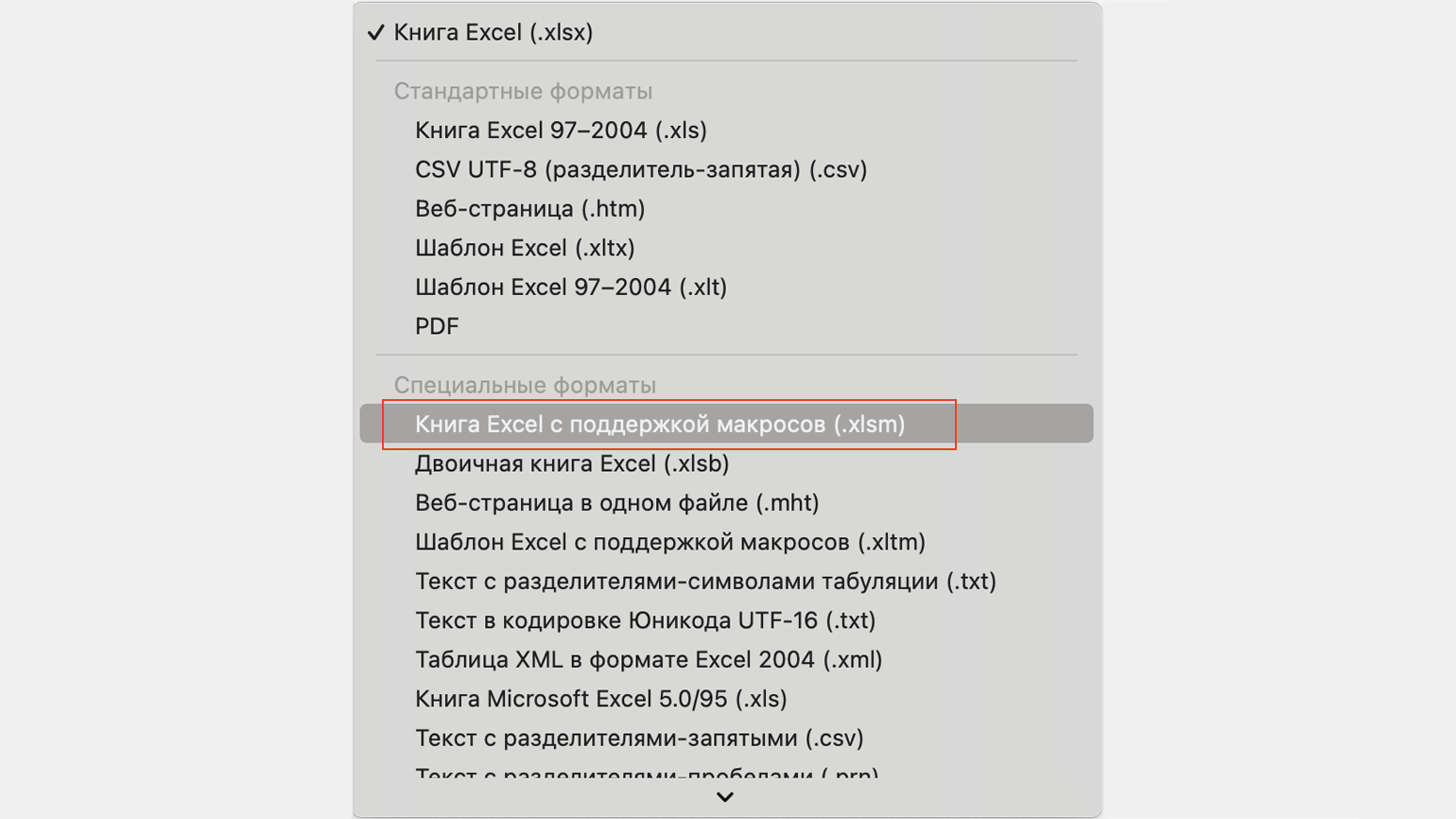
Скриншот: Skillbox Media
Перед началом записи макроса важно знать об особенностях его работы:
- Макрос записывает все действия пользователя.
После старта записи макрос начнёт регистрировать все клики мышки и все нажатия клавиш. Поэтому перед записью последовательности лучше хорошо отработать её, чтобы не добавлять лишних действий и не удлинять код. Если требуется записать длинную последовательность задач — лучше разбить её на несколько коротких и записать несколько макросов.
- Работу макроса нельзя отменить.
Все действия, которые выполняет запущенный макрос, остаются в файле навсегда. Поэтому перед тем, как запускать макрос в первый раз, лучше создать копию всего файла. Если что-то пойдёт не так, можно будет просто закрыть его и переписать макрос в созданной копии.
- Макрос выполняет свой алгоритм только для записанного диапазона таблиц.
Если при записи макроса пользователь выбирал диапазон таблицы, то и при запуске макроса в другом месте он выполнит свой алгоритм только в рамках этого диапазона. Если добавить новую строку, макрос к ней применяться не будет. Поэтому при записи макроса можно сразу выбирать большее количество строк — как это сделать, показываем ниже.
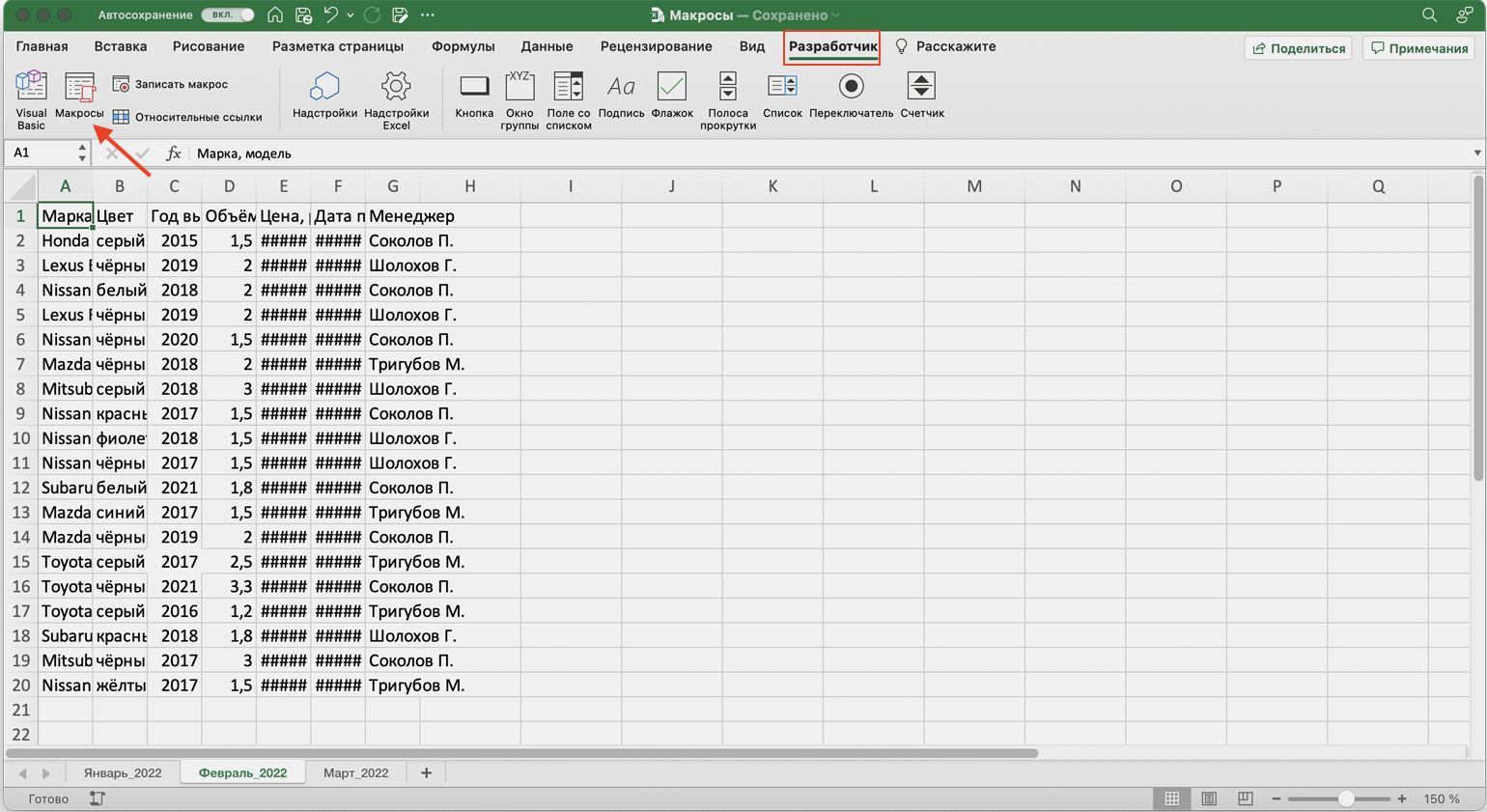
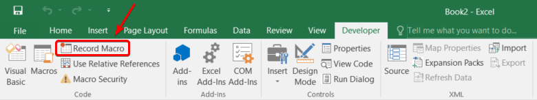
Для начала записи макроса перейдём на вкладку «Разработчик» и нажмём кнопку «Записать макрос».
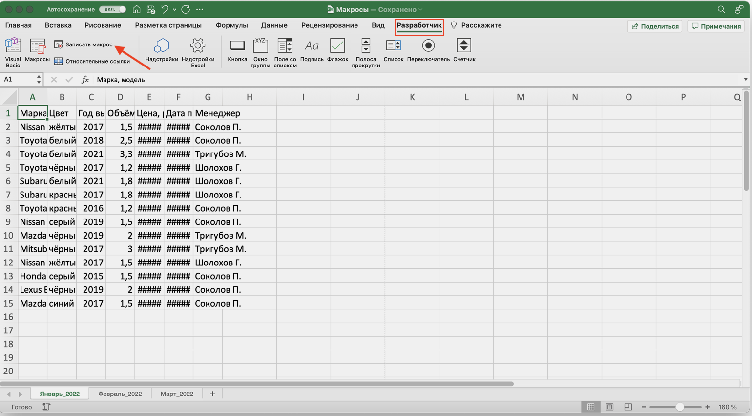
Скриншот: Skillbox Media
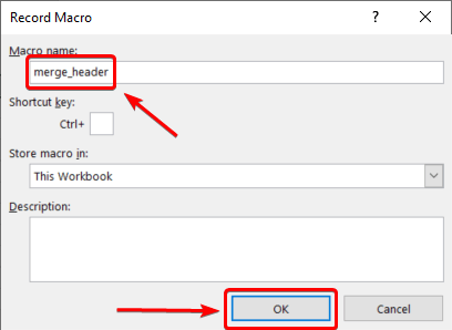
Появляется окно для заполнения параметров макроса. Нужно заполнить поля: «Имя макроса», «Сохранить в», «Сочетание клавиш», «Описание».
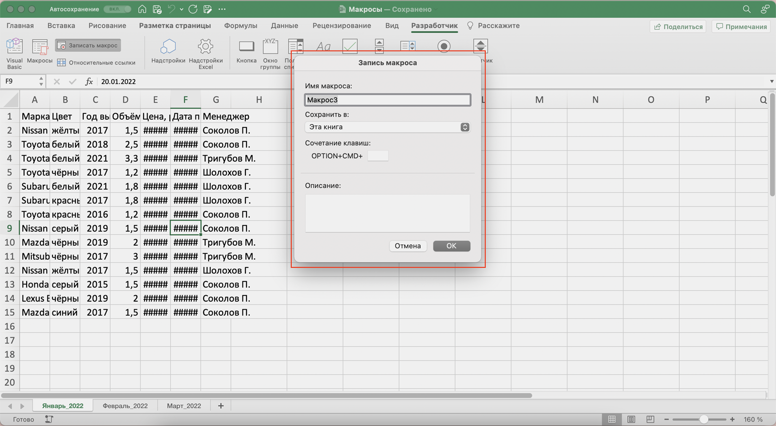
Скриншот: Skillbox Media
«Имя макроса» — здесь нужно придумать и ввести название для макроса. Лучше сделать его логически понятным, чтобы в дальнейшем можно было быстро его найти.
Первым символом в названии обязательно должна быть буква. Другие символы могут быть буквами или цифрами. Важно не использовать пробелы в названии — их можно заменить символом подчёркивания.
«Сохранить в» — здесь нужно выбрать книгу, в которую макрос сохранится после записи.
Если выбрать параметр «Эта книга», макрос будет доступен при работе только в этом файле Excel. Чтобы макрос был доступен всегда, нужно выбрать параметр «Личная книга макросов» — Excel создаст личную книгу макросов и сохранит новый макрос в неё.
«Сочетание клавиш» — здесь к уже выбранным двум клавишам (Ctrl + Shift в системе Windows и Option + Cmd в системе macOS) нужно добавить третью клавишу. Это должна быть строчная или прописная буква, которую ещё не используют в других быстрых командах компьютера или программы Excel.
В дальнейшем при нажатии этих трёх клавиш записанный макрос будет запускаться автоматически.
«Описание» — необязательное поле, но лучше его заполнять. Например, можно ввести туда последовательность действий, которые планируется записать в этом макросе. Так не придётся вспоминать, какие именно команды выполнит этот макрос, если нужно будет запустить его позже. Плюс будет проще ориентироваться среди других макросов.
В нашем случае с форматированием таблицы заполним поля записи макроса следующим образом и нажмём «ОК».
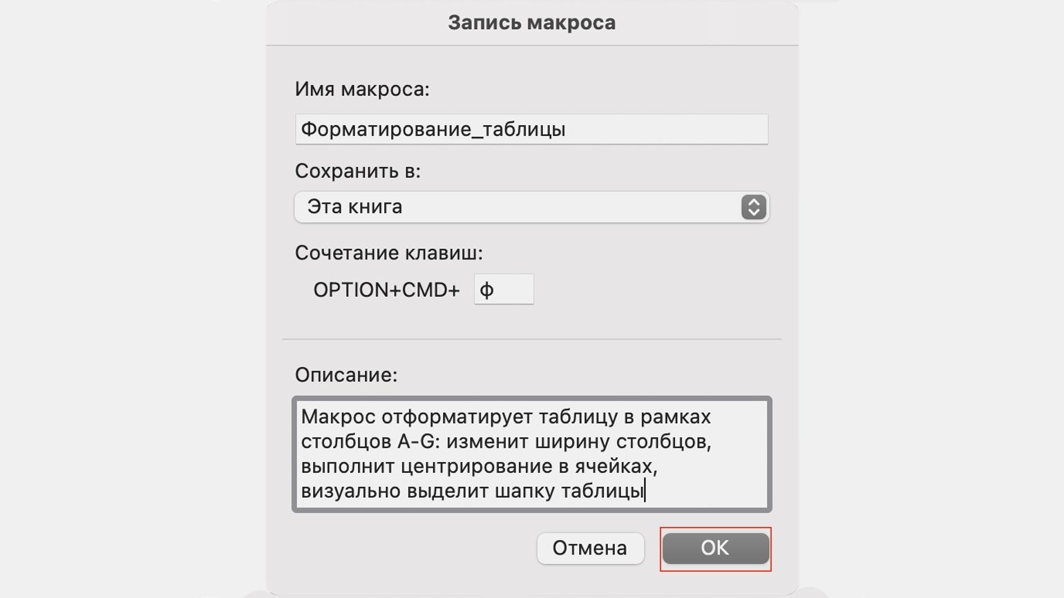
Скриншот: Skillbox Media
После этого начнётся запись макроса — в нижнем левом углу окна Excel появится значок записи.
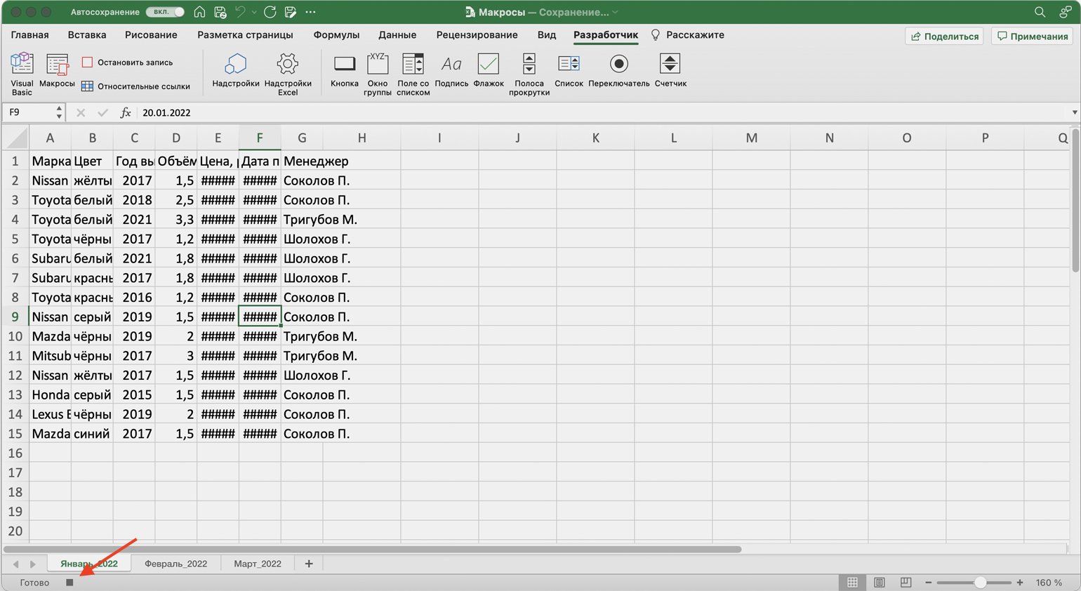
Скриншот: Skillbox Media
Пока идёт запись, форматируем таблицу с продажами за январь: меняем ширину всех столбцов, данные во всех ячейках располагаем по центру, выделяем шапку таблицы цветом и жирным шрифтом, рисуем границы.
Важно: в нашем случае у таблиц продаж за январь, февраль и март одинаковое количество столбцов, но разное количество строк. Чтобы в случае со второй и третьей таблицей макрос сработал корректно, при форматировании выделим диапазон так, чтобы в него попали не только строки самой таблицы, но и строки ниже неё. Для этого нужно выделить столбцы в строке с их буквенным обозначением A–G, как на рисунке ниже.
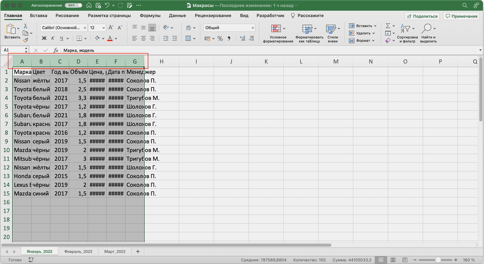
Скриншот: Skillbox Media
Если выбрать диапазон только в рамках первой таблицы, то после запуска макроса в таблице с большим количеством строк она отформатируется только частично.
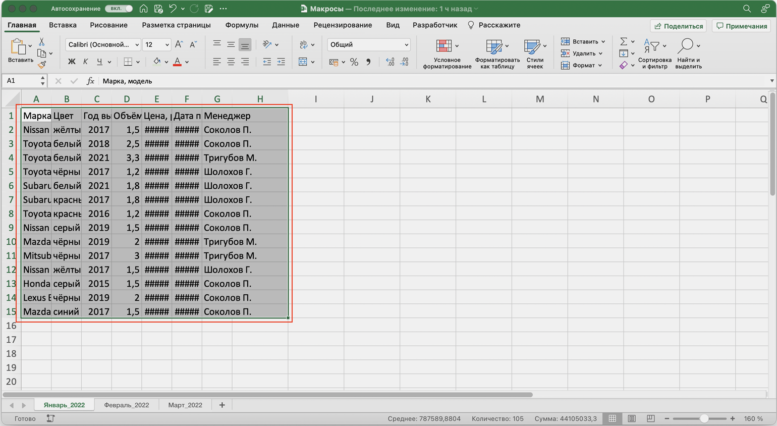
Скриншот: Skillbox Media
После всех манипуляций с оформлением таблица примет такой вид:
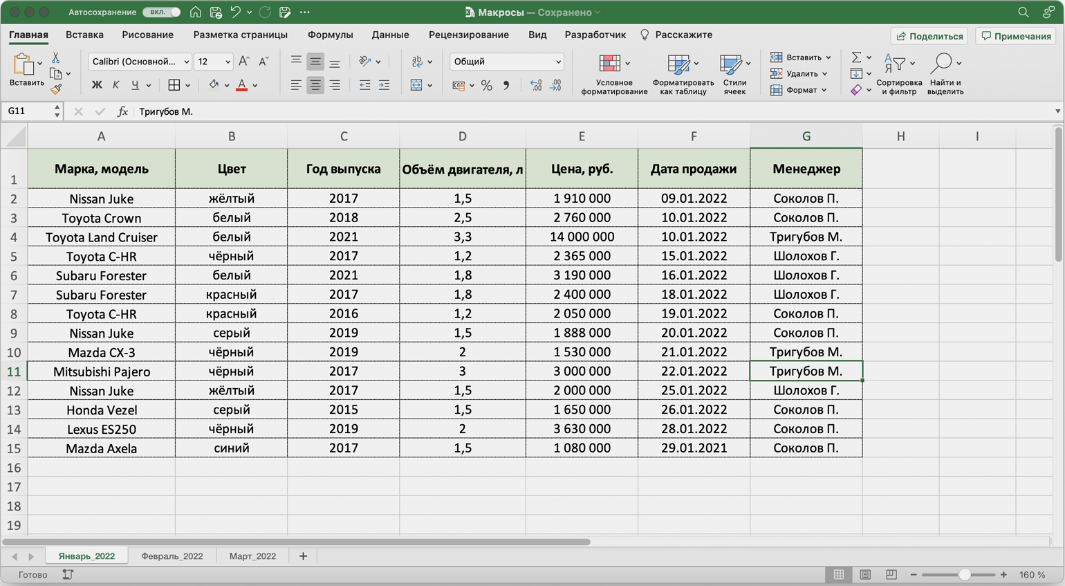
Скриншот: Skillbox Media
Проверяем, все ли действия с таблицей мы выполнили, и останавливаем запись макроса. Сделать это можно двумя способами:
- Нажать на кнопку записи в нижнем левом углу.
- Перейти во вкладку «Разработчик» и нажать кнопку «Остановить запись».
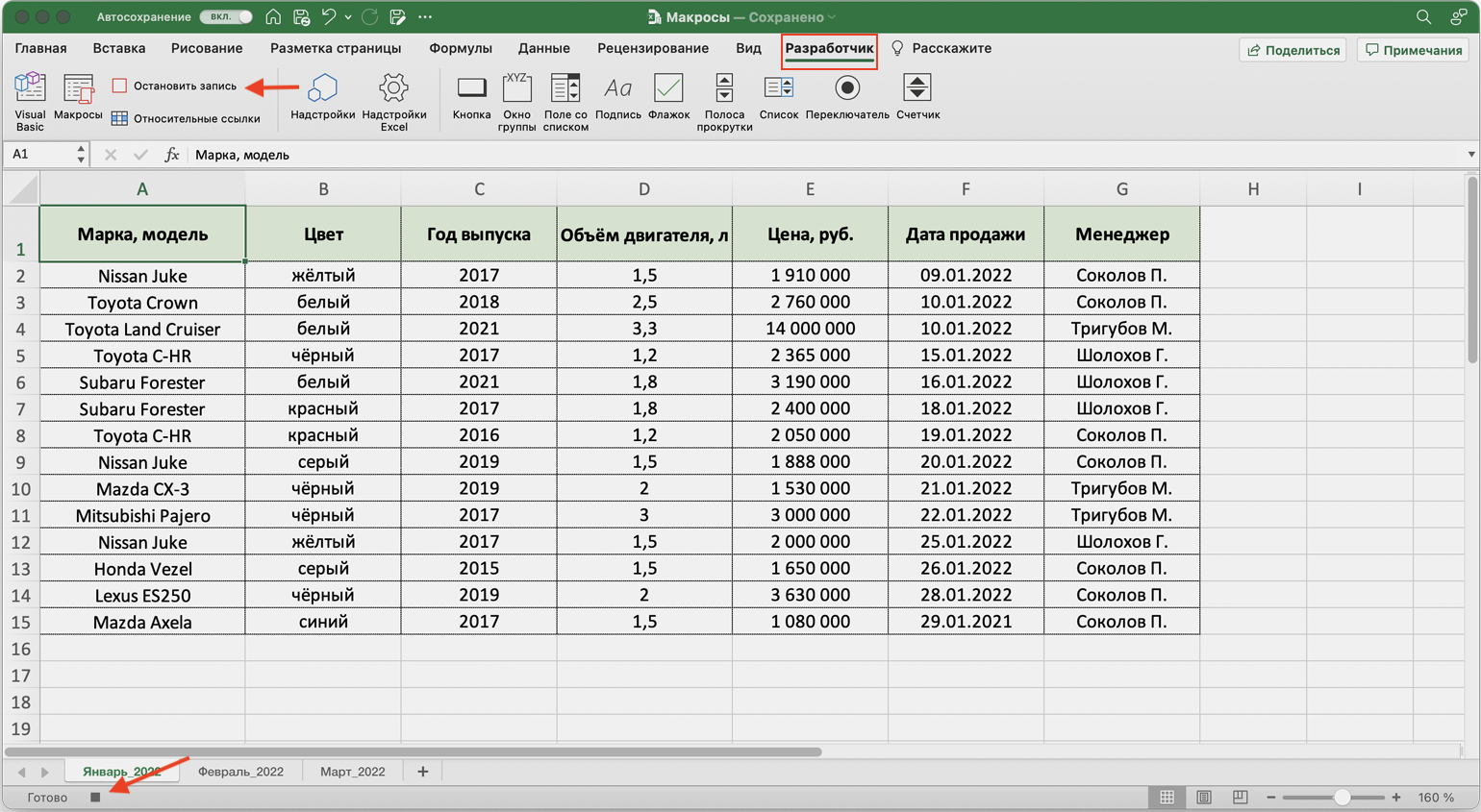
Скриншот: Skillbox Media
Готово — мы создали макрос для форматирования таблиц в границах столбцов A–G. Теперь его можно применить к другим таблицам.
Запускаем макрос
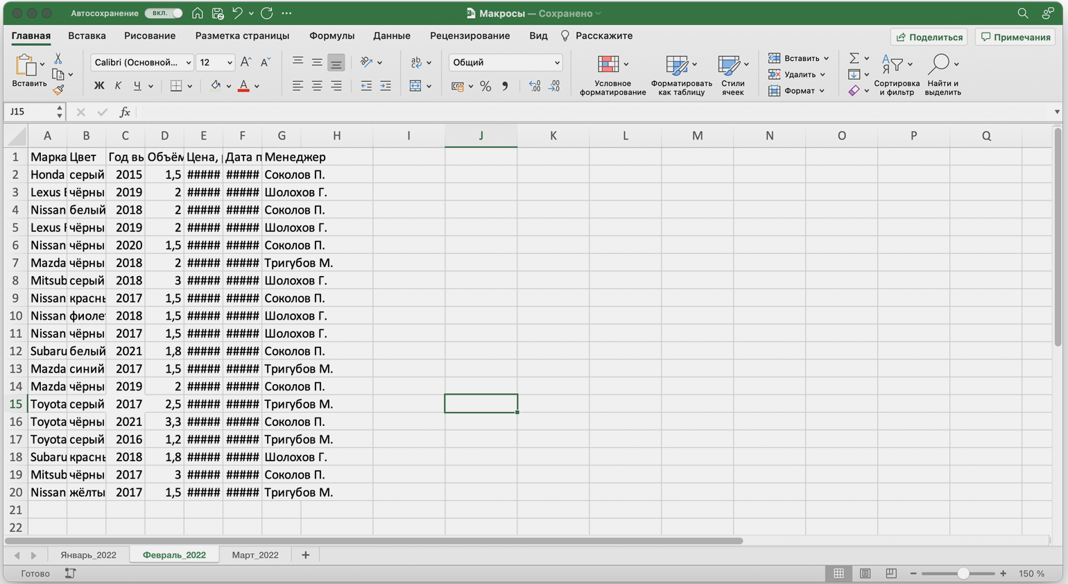
Перейдём в лист со второй таблицей «Февраль_2022». В первоначальном виде она такая же нечитаемая, как и первая таблица до форматирования.
Скриншот: Skillbox Media
Отформатируем её с помощью записанного макроса. Запустить макрос можно двумя способами:
- Нажать комбинацию клавиш, которую выбрали при заполнении параметров макроса — в нашем случае Option + Cmd + Ф.
- Перейти во вкладку «Разработчик» и нажать кнопку «Макросы».
Скриншот: Skillbox Media
Появляется окно — там выбираем макрос, который нужно запустить. В нашем случае он один — «Форматирование_таблицы». Под ним отображается описание того, какие действия он включает. Нажимаем «Выполнить».
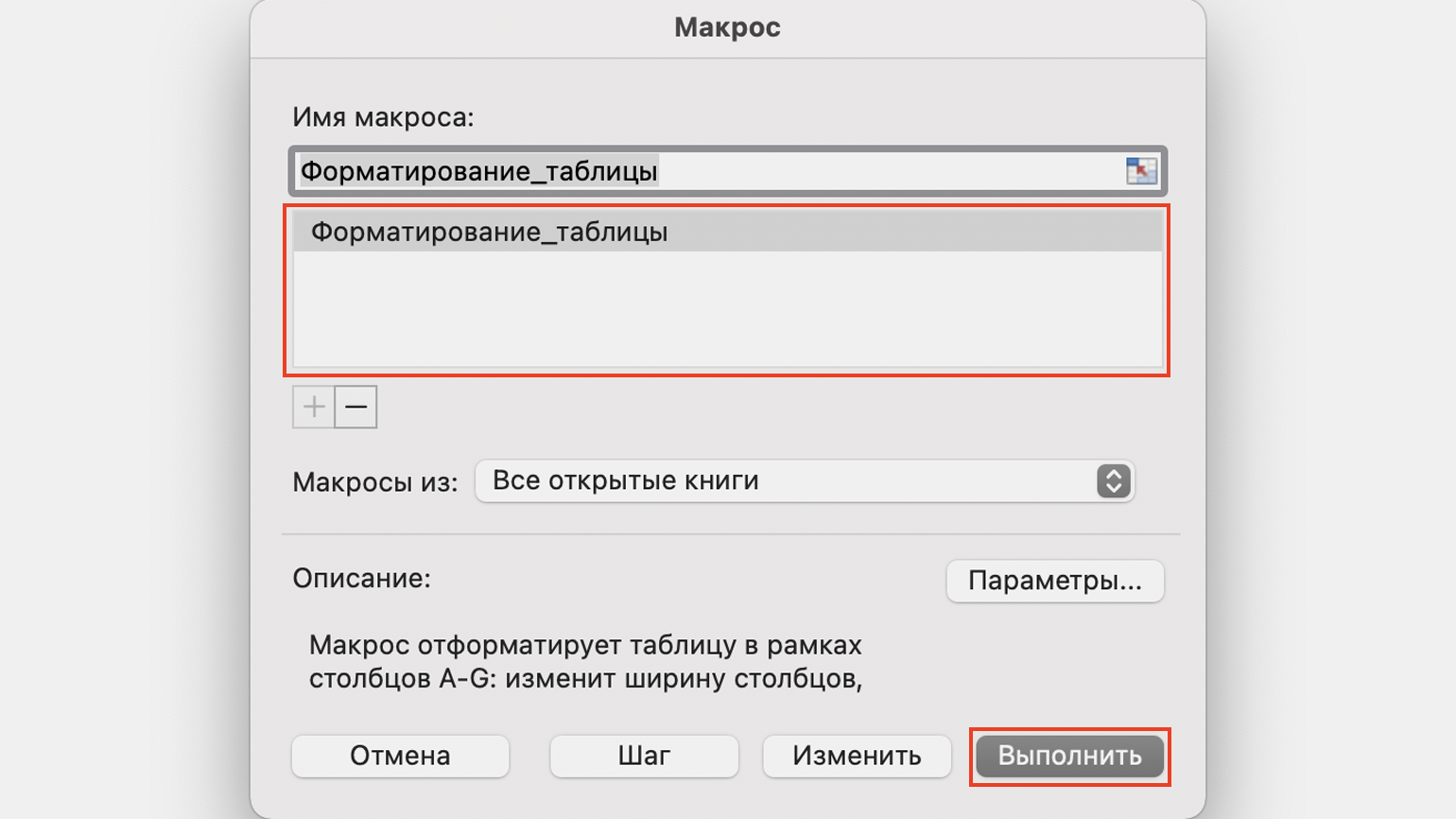
Скриншот: Skillbox Media
Готово — вторая таблица с помощью макроса форматируется так же, как и первая.
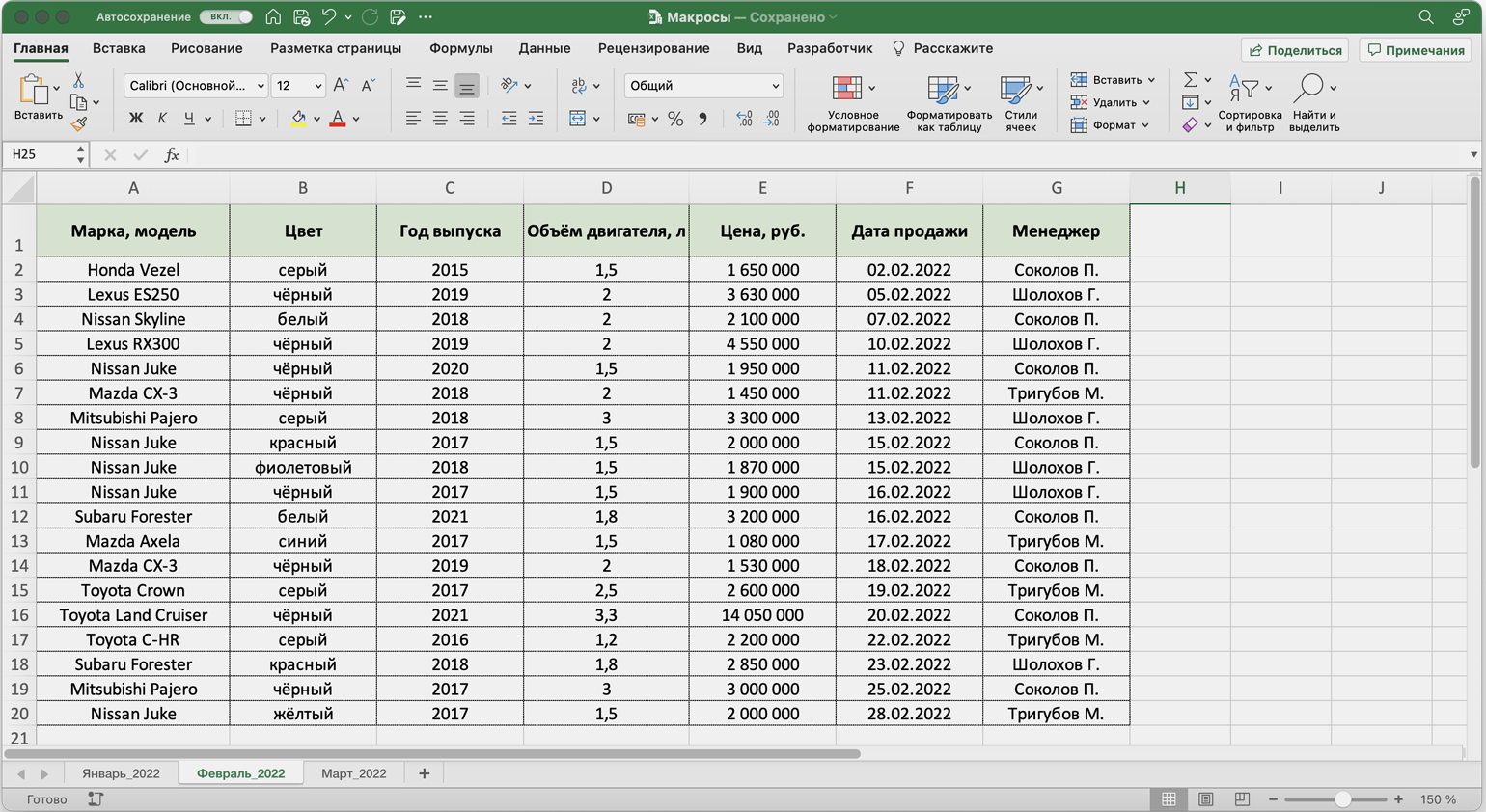
Скриншот: Skillbox Media
То же самое можно сделать и на третьем листе для таблицы продаж за март. Более того, этот же макрос можно будет запустить и в следующем квартале, когда сервис автосалона выгрузит таблицы с новыми данными.

Научитесь: Excel + Google Таблицы с нуля до PRO
Узнать больше
![]()
Download Article
![]()
Download Article
While Excel is full of time-saving features like keyboard shortcuts and templates, you can save even more time by creating macros to complete repetitive tasks. This wikiHow teaches how to create simple macros for Excel spreadsheets.
-
1
Open Excel. The process for showing the Developer tab is the same for many versions of Excel for Windows. There is a slight difference for Excel for Mac, which will be detailed below.
-
2
Click the File tab. It’s in the editing ribbon above your document space.
- In Excel for Mac, click the «Excel» menu at the top of your screen.
Advertisement
-
3
Click Options. You might find this option at the bottom of the menu.
- In Excel for Mac, click the «Preferences» menu option.
-
4
Click Customize Ribbon. It’s in the panel on the left side of the window.
- In Excel for Mac, click «Ribbon & Toolbar» in the «Authoring» section.
-
5
Check the box next to «Developer» to check it. You’ll see this on the right side of the window under the header, «Main Tabs.»
- In Excel for Mac, you’ll see «Developer» in the «Tab or Group Title» list.
-
6
Click OK. You’ll see the Developer tab appear in your tab list.


Advertisement
-
1
Click the Developer tab.You should see this in the editing ribbon above your editing space. If you don’t see it, you need to enable it again.
-
2
Click Record Macro. You’ll find this in the Code section of the Developer tab. You can also press Alt+T+M+R to start a new macro (Windows only).
-
3
Give the macro a name. Make sure that you’ll be able to easily identify it, especially if you’re going to be creating multiple macros.
- You can also add a description to explain what the macro will accomplish.
-
4
Click the Shortcut key field. You can assign a keyboard shortcut to the macro to easily run it. This is optional.
-
5
Press ⇧ Shift plus a letter. This will create a Ctrl+⇧ Shift+letter keyboard combination to start the macro. If you don’t press Shift, then you run the risk of overwriting any keyboard shortcuts that already exist. For instance, if you entered z in the box without pressing Shift, you’d overwrite the «Undo» shortcut (which is Ctrl + Z)
- On Mac, this will be a ⌥ Opt+⌘ Command+letter combination.
-
6
Click the Store macro in drop-down. More options will drop down for you.
-
7
Click the location you want to save the macro. If you’re only using the macro for your current spreadsheet, just leave it on «This Workbook.» If you want the macro available for any spreadsheet you work on, select «Personal Macro Workbook.»
-
8
Click OK. Your macro will begin recording.
-
9
Perform the commands you want to record. Pretty much anything you do will now be recorded and added to the macro. For example, if you run a sum formula of A2 and B2 in cell C7, running the macro in the future will always sum A2 and B2 and display the results in C7.
- Macros can get very complex, and you can even use them to open other Office programs. When the macro is recording, virtually everything you do in Excel is added to the macro.[1]
- Macros can get very complex, and you can even use them to open other Office programs. When the macro is recording, virtually everything you do in Excel is added to the macro.[1]
-
10
Click Stop Recording when you’re finished. This will end the macro recording and save it.
-
11
Save your file in a macro-enabled format. In order to preserve your macros, you’ll need to save your workbook as a special macro-enabled Excel format:
- Click the File menu and select Save.
- Click the File Type menu underneath the file name field.
- Click Excel Macro-Enabled Workbook.


Advertisement
-
1
Open your macro-enabled workbook file. If you have closed your file before running your macro, you’ll be prompted to enable the content.
-
2
Click Enable Content. This appears at the top of the Excel spreadsheet in a Security Warning bar whenever a macro-enabled workbook is opened. Since it’s your own file, you can trust it, but be very careful opening macro-enabled files from any other source.
-
3
Press your macro shortcut (if you want to use a shortcut key). When you want to use your macro, you can quickly run it by pressing the shortcut you created for it.
-
4
Click the Macros button in the Developer tab (if you want to use the menu). This will display all of the macros that are available in your current spreadsheet.
-
5
Click the macro you want to run.
-
6
Click the Run button (if you have custom buttons enabled). The macro will be run in your current cell or selection.
- If you don’t have custom buttons enabled, you can go to Customize Ribbon and add it there.[2]
- If you don’t have custom buttons enabled, you can go to Customize Ribbon and add it there.[2]
-
7
View a macro’s code. If you want to learn more about how macro coding works, you can open the code of any macro you’ve created and tinker with it:
- Click the Macros button in the Developer tab.
- Click the macro you want to view.
- Click the Edit button.
- View your macro code in the Visual Basic code editing window.


Advertisement
Add New Question
-
Question
If I have two lines of dates in one cell, how do I delete the first line?

Double click on the cell, or click the cell and then F2. Then, delete the part that you don’t need. If you want to do this on a large number of cells on the same column, then select the column, click «DATA» on the top menu, click on «Text to Columns,» and try the different options to divide the data there. (There are too many to list here.) You can divide by commas, spaces, dashes, periods, etc., or specify the length. Make sure the columns on the right are empty; the divided data will split into those columns.
-
Question
While recording a macro, will it record something I want done outside of Excel, such as opening up a website and clicking on things in that website?
No. The macro program in Excel is limited to Excel. Once you use an outside program, Excel will be unable to record what you are doing.
-
Question
How do I secure files in Excel?
Click the Microsoft Office button, point to Prepare, and then click Encrypt Document.
In the Password box, type a password, and then click OK.
In the Reenter Password box, type the password again, and then click OK.
To save the password, save the file.
See more answers
Ask a Question
200 characters left
Include your email address to get a message when this question is answered.
Submit
Advertisement
Thanks for submitting a tip for review!
About This Article
Article SummaryX
1. Enable macros.
2. Click the Developer tab.
3. Click Record Macro.
4. Name the macro.
5. Specify a shortcut key.
6. Select This Workbook under “Store macro in.”
7. Click OK.
8. Perform the commands you want to record.
9. Click Stop Recording when finished.
10. Save the file as a Macro-Enabled Workbook (*.xlsm).
Did this summary help you?
Thanks to all authors for creating a page that has been read 1,598,511 times.
Is this article up to date?
Введение
Всем нам приходится — кому реже, кому чаще — повторять одни и те же действия и операции в Excel. Любая офисная работа предполагает некую «рутинную составляющую» — одни и те же еженедельные отчеты, одни и те же действия по обработке поступивших данных, заполнение однообразных таблиц или бланков и т.д. Использование макросов и пользовательских функций позволяет автоматизировать эти операции, перекладывая монотонную однообразную работу на плечи Excel. Другим поводом для использования макросов в вашей работе может стать необходимость добавить в Microsoft Excel недостающие, но нужные вам функции. Например функцию сборки данных с разных листов на один итоговый лист, разнесения данных обратно, вывод суммы прописью и т.д.
Макрос — это запрограммированная последовательность действий (программа, процедура), записанная на языке программирования Visual Basic for Applications (VBA). Мы можем запускать макрос сколько угодно раз, заставляя Excel выполнять последовательность любых нужных нам действий, которые нам не хочется выполнять вручную.
В принципе, существует великое множество языков программирования (Pascal, Fortran, C++, C#, Java, ASP, PHP…), но для всех программ пакета Microsoft Office стандартом является именно встроенный язык VBA. Команды этого языка понимает любое офисное приложение, будь то Excel, Word, Outlook или Access.
Способ 1. Создание макросов в редакторе Visual Basic
Для ввода команд и формирования программы, т.е. создания макроса необходимо открыть специальное окно — редактор программ на VBA, встроенный в Microsoft Excel.
- В старых версиях (Excel 2003 и старше) для этого идем в меню Сервис — Макрос — Редактор Visual Basic (Toos — Macro — Visual Basic Editor).
- В новых версиях (Excel 2007 и новее) для этого нужно сначала отобразить вкладку Разработчик (Developer). Выбираем Файл — Параметры — Настройка ленты (File — Options — Customize Ribbon) и включаем в правой части окна флажок Разработчик (Developer). Теперь на появившейся вкладке нам будут доступны основные инструменты для работы с макросами, в том числе и нужная нам кнопка Редактор Visual Basic (Visual Basic Editor)
 :
:
 :
:К сожалению, интерфейс редактора VBA и файлы справки не переводятся компанией Microsoft на русский язык, поэтому с английскими командами в меню и окнах придется смириться:

Макросы (т.е. наборы команд на языке VBA) хранятся в программных модулях. В любой книге Excel мы можем создать любое количество программных модулей и разместить там наши макросы. Один модуль может содержать любое количество макросов. Доступ ко всем модулям осуществляется с помощью окна Project Explorer в левом верхнем углу редактора (если его не видно, нажмите CTRL+R). Программные модули бывают нескольких типов для разных ситуаций:
- Обычные модули — используются в большинстве случаев, когда речь идет о макросах. Для создания такого модуля выберите в меню Insert — Module. В появившееся окно нового пустого модуля можно вводить команды на VBA, набирая их с клавиатуры или копируя их из другого модуля, с этого сайта или еще откуда нибудь:

- Модуль Эта книга — также виден в левом верхнем углу редактора Visual Basic в окне, которое называется Project Explorer. В этот модуль обычно записываются макросы, которые должны выполнятся при наступлении каких-либо событий в книге (открытие или сохранение книги, печать файла и т.п.):

- Модуль листа — доступен через Project Explorer и через контекстное меню листа, т.е. правой кнопкой мыши по ярлычку листа — команда Исходный текст (View Source). Сюда записывают макросы, которые должны выполняться при наступлении определенных событий на листе (изменение данных в ячейках, пересчет листа, копирование или удаление листа и т.д.)


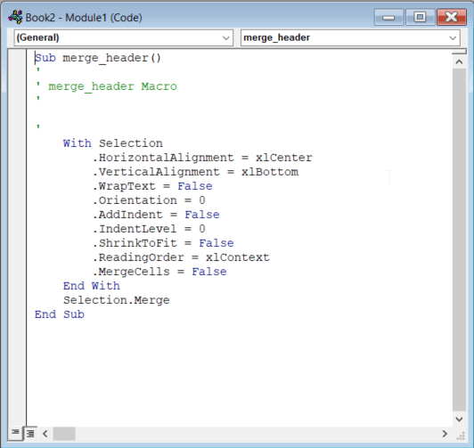
Обычный макрос, введенный в стандартный модуль выглядит примерно так:

Давайте разберем приведенный выше в качестве примера макрос Zamena:
- Любой макрос должен начинаться с оператора Sub, за которым идет имя макроса и список аргументов (входных значений) в скобках. Если аргументов нет, то скобки надо оставить пустыми.
- Любой макрос должен заканчиваться оператором End Sub.
- Все, что находится между Sub и End Sub — тело макроса, т.е. команды, которые будут выполняться при запуске макроса. В данном случае макрос выделяет ячейку заливает выделенных диапазон (Selection) желтым цветом (код = 6) и затем проходит в цикле по всем ячейкам, заменяя формулы на значения. В конце выводится окно сообщения (MsgBox).
С ходу ясно, что вот так сразу, без предварительной подготовки и опыта в программировании вообще и на VBA в частности, сложновато будет сообразить какие именно команды и как надо вводить, чтобы макрос автоматически выполнял все действия, которые, например, Вы делаете для создания еженедельного отчета для руководства компании. Поэтому мы переходим ко второму способу создания макросов, а именно…
Способ 2. Запись макросов макрорекордером
Макрорекордер — это небольшая программа, встроенная в Excel, которая переводит любое действие пользователя на язык программирования VBA и записывает получившуюся команду в программный модуль. Если мы включим макрорекордер на запись, а затем начнем создавать свой еженедельный отчет, то макрорекордер начнет записывать команды вслед за каждым нашим действием и, в итоге, мы получим макрос создающий отчет как если бы он был написан программистом. Такой способ создания макросов не требует знаний пользователя о программировании и VBA и позволяет пользоваться макросами как неким аналогом видеозаписи: включил запись, выполнил операци, перемотал пленку и запустил выполнение тех же действий еще раз. Естественно у такого способа есть свои плюсы и минусы:
- Макрорекордер записывает только те действия, которые выполняются в пределах окна Microsoft Excel. Как только вы закрываете Excel или переключаетесь в другую программу — запись останавливается.
- Макрорекордер может записать только те действия, для которых есть команды меню или кнопки в Excel. Программист же может написать макрос, который делает то, что Excel никогда не умел (сортировку по цвету, например или что-то подобное).
- Если во время записи макроса макрорекордером вы ошиблись — ошибка будет записана. Однако смело можете давить на кнопку отмены последнего действия (Undo) — во время записи макроса макрорекордером она не просто возрвращает Вас в предыдущее состояние, но и стирает последнюю записанную команду на VBA.
Чтобы включить запись необходимо:
- в Excel 2003 и старше — выбрать в меню Сервис — Макрос — Начать запись (Tools — Macro — Record New Macro)
- в Excel 2007 и новее — нажать кнопку Запись макроса (Record macro) на вкладке Разработчик (Developer)
Затем необходимо настроить параметры записываемого макроса в окне Запись макроса:

- Имя макроса — подойдет любое имя на русском или английском языке. Имя должно начинаться с буквы и не содержать пробелов и знаков препинания.
- Сочетание клавиш — будет потом использоваться для быстрого запуска макроса. Если забудете сочетание или вообще его не введете, то макрос можно будет запустить через меню Сервис — Макрос — Макросы — Выполнить (Tools — Macro — Macros — Run) или с помощью кнопки Макросы (Macros) на вкладке Разработчик (Developer) или нажав ALT+F8.
- Сохранить в… — здесь задается место, куда будет сохранен текст макроса, т.е. набор команд на VBA из которых и состоит макрос.:
- Эта книга — макрос сохраняется в модуль текущей книги и, как следствие, будет выполнятся только пока эта книга открыта в Excel
- Новая книга — макрос сохраняется в шаблон, на основе которого создается любая новая пустая книга в Excel, т.е. макрос будет содержаться во всех новых книгах, создаваемых на данном компьютере начиная с текущего момента
- Личная книга макросов — это специальная книга Excel с именем Personal.xls, которая используется как хранилище макросов. Все макросы из Personal.xls загружаются в память при старте Excel и могут быть запущены в любой момент и в любой книге.
После включения записи и выполнения действий, которые необходимо записать, запись можно остановить командой Остановить запись (Stop Recording).
Запуск и редактирование макросов
Управление всеми доступными макросами производится в окне, которое можно открыть с помощью кнопки Макросы (Macros) на вкладке Разработчик (Developer) или — в старых версиях Excel — через меню Сервис — Макрос — Макросы (Tools — Macro — Macros):

- Любой выделенный в списке макрос можно запустить кнопкой Выполнить (Run).
- Кнопка Параметры (Options) позволяет посмотреть и отредактировать сочетание клавиш для быстрого запуска макроса.
- Кнопка Изменить (Edit) открывает редактор Visual Basic (см. выше) и позволяет просмотреть и отредактировать текст макроса на VBA.
Создание кнопки для запуска макросов
Чтобы не запоминать сочетание клавиш для запуска макроса, лучше создать кнопку и назначить ей нужный макрос. Кнопка может быть нескольких типов:
Кнопка на панели инструментов в Excel 2003 и старше
Откройте меню Сервис — Настройка (Tools — Customize) и перейдите на вкладку Команды (Commands). В категории Макросы легко найти веселый желтый «колобок» — Настраиваемую кнопку (Custom button):

Перетащите ее к себе на панель инструментов и затем щелкните по ней правой кнопкой мыши. В контекстом меню можно назначить кнопке макрос, выбрать другой значок и имя:

Кнопка на панели быстрого доступа в Excel 2007 и новее
Щелкните правой кнопкой мыши по панели быстрого доступа в левом верхнем углу окна Excel и выберите команду Настройка панели быстрого доступа (Customise Quick Access Toolbar):

Затем в открывшемся окне выберите категорию Макросы и при помощи кнопки Добавить (Add) перенесите выбранный макрос в правую половину окна, т.е. на панель быстрого доступа:

Кнопка на листе
Этот способ подходит для любой версии Excel. Мы добавим кнопку запуска макроса прямо на рабочий лист, как графический объект. Для этого:
- В Excel 2003 и старше — откройте панель инструментов Формы через меню Вид — Панели инструментов — Формы (View — Toolbars — Forms)
- В Excel 2007 и новее — откройте выпадающий список Вставить (Insert) на вкладке Разработчик (Developer)
Выберите объект Кнопка (Button):

Затем нарисуйте кнопку на листе, удерживая левую кнопку мыши. Автоматически появится окно, где нужно выбрать макрос, который должен запускаться при щелчке по нарисованной кнопке.
Создание пользовательских функций на VBA
Создание пользовательских функций или, как их иногда еще называют, UDF-функций (User Defined Functions) принципиально не отличается от создания макроса в обычном программном модуле. Разница только в том, что макрос выполняет последовательность действий с объектами книги (ячейками, формулами и значениями, листами, диаграммами и т.д.), а пользовательская функция — только с теми значениями, которые мы передадим ей как аргументы (исходные данные для расчета).
Чтобы создать пользовательскую функцию для расчета, например, налога на добавленную стоимость (НДС) откроем редактор VBA, добавим новый модуль через меню Insert — Module и введем туда текст нашей функции:

Обратите внимание, что в отличие от макросов функции имеют заголовок Function вместо Sub и непустой список аргументов (в нашем случае это Summa). После ввода кода наша функция становится доступна в обычном окне Мастера функций (Вставка — Функция) в категории Определенные пользователем (User Defined):

После выбора функции выделяем ячейки с аргументами (с суммой, для которой надо посчитать НДС) как в случае с обычной функцией:

You work in Excel every day and do the same things again and again. Why not automate those tasks? Or, maybe, you want Excel to do most of the work for you? Read on to learn what Excel macros are and how they can help you.
What are macros in Excel?
Excel is an extremely powerful tool for processing data in the form of spreadsheets. While most users use formulas, there is another way to manipulate data in Excel.
Excel macros are pieces of code that describe specific actions or contain a set of instructions. Every time you launch the macro, Excel follows those instructions step-by-step.
Why learn macros in Excel?
Macros are a must-have tool for an advanced Excel user. By using Excel macros you can avoid dull, repetitive actions or even create your own order management system for free.
Simple macros in Excel that will make things easier
There are lots of simple Excel macros that take just a few lines of code, but can save you hours. Excel can perform certain operations instantly, where it would take you a very long time to do the job manually.
For example, this macro will sort all worksheets alphabetically:
Sub SortSheetsTabName()
Application.ScreenUpdating = False
Dim ShCount As Integer, i As Integer, j As Integer
ShCount = Sheets.Count
For i = 1 To ShCount - 1
For j = i + 1 To ShCount
If Sheets(j).Name < Sheets(i).Name Then
Sheets(j).Move before:=Sheets(i)
End If
Next j
Next i
Application.ScreenUpdating = True
End Sub
The following code will unhide all hidden worksheets:
Sub UnhideAllWoksheets()
Dim ws As Worksheet
For Each ws In ActiveWorkbook.Worksheets
ws.Visible = xlSheetVisible
Next ws
End Sub
To unhide all rows and columns on a worksheet, use:
Sub UnhideRowsColumns()
Columns.EntireColumn.Hidden = False
Rows.EntireRow.Hidden = False
End Sub
Advanced Excel macros that can significantly improve your workflow
If you are running a business, you have to store and manipulate data. Small companies can keep records by hand and large enterprises can buy specialized software (which is rather expensive). But what about medium-sized businesses that can no longer settle for manual record-keeping, but still cannot afford costly software? This is where Excel with macros shines.
By combining advanced Excel macros you can create a CRM (Customer Relationship Management) system which will help you provide better services. If you sell goods, you need an inventory management tool and Excel spreadsheets enhanced with macros will fit your needs.
If your data is contained in multiple Excel workbooks, you can use Coupler.io to move them around. You can even add third-party sources, like Google Sheets, Airtable, BigQuery, etc. Data integration with Coupler.io does not require any programming skills and can be done in just a few clicks.
Check out the available integrations with Excel.
Other Excel macros examples
Below are a few examples of useful Excel macros.
Sometimes you might accidentally add extra spaces to the data in cells. This mistake will cause errors, thereby preventing you from making correct calculations. To remove unnecessary spaces from the selected cells, use the following code:
Sub TrimTheSpaces()
Dim MyRange As Range
Dim MyCell As Range
Set MyRange = Selection
For Each MyCell In MyRange
If Not IsEmpty(MyCell) Then
MyCell = Trim(MyCell)
End If
Next MyCell
End Sub
It is often the case that you need to protect your workbook with a password. You can do that in the user interface of Excel. However, if you use the same password for all of your workbooks, you have to re-enter it every time. This macro will do the job for you (don’t forget to replace “1234” with your own password!):
Sub ProtectSheets()
Dim ws As Worksheet
For Each ws In ActiveWorkbook.Worksheets
ws.Protect Password:="1234"
Next ws
End Sub
Using macros in Excel
As macros are programs that can do literally anything on your computer, using macros from untrusted sources is very risky. That’s why, when you open a workbook with macros in Excel, they will be disabled and you will see the following notification:
![]()
If you trust the source of the file, click Enable Content. That will add the workbook to the list of trusted documents and turn on its macros. The next time you open that workbook, there will be no warning.
You will see the above notification each time you open a workbook if it has been saved to an untrusted location. That can be a folder for temporary files or browser downloads. To avoid that, move the file to another folder or enable macros in the Excel Trust Center.
How to enable macros in Excel
If you do not want to see the security warning when opening Excel workbooks, you can permanently enable macros in the Trust Center.
To enable macros in the Excel Trust Center:
- In the upper-left corner, click the File tab and then select Options:

- In the Excel Options window, select Trust Center and then click Trust Center Settings:

- In the Trust Center, go to Macro Settings and then select Enable all macros:

Warning! Enabling macros for all workbooks is potentially risky because files from external sources may contain malicious code. If you open such a workbook, the macros may run automatically and corrupt your data or even cause hardware malfunctions.
How to use macros in Excel
If your workbook contains macros, you can run them by pressing Alt+F8. In the Macro window that opens, select the macro you need and click Run:

If you want to create new macros, you need to enable the Developer tab first.
To enable the Developer tab:
- In the upper-left corner, click the File tab and then select Options.
- In the Excel Options window, select Customize Ribbon and then enable the Developer checkbox in the Main Tabs area:

- Click OK to apply the changes.
In the Developer tab you can run existing macros by clicking the Macros button or create a new macro. For details on creating macros in Excel, see the following sections.

How to delete macros in Excel
To delete a macro in Excel:
- Open the Macro window in one of the following ways:
- Press Alt+F8.
- Select the Developer tab and click Macros.
- Select the macro that you want to delete and click Delete.

- Click Yes in the confirmation window that opens.
How to disable macros in Excel
Enabling Excel macros can make your computer vulnerable. Some macros will run when you open a workbook, which is especially dangerous if you have downloaded the workbook from an untrusted source. To prevent that, you can disable macros in Excel either with or without a notification.
To disable macros in Excel:
- In the upper-left corner, click the File tab and then select Options.
- In the Excel Options window, select Trust Center and then click Trust Center Settings.
- In the Trust Center, go to Macro Settings and then select one of the following options:
- Disable all macros without notification. Macros will be disabled and you will not see a security warning when opening a workbook with macros.
- Disable all macros with notification. Macros will be disabled but you will see a security warning when opening a workbook with macros and will be able to allow macros, if needed.

Writing macros in Excel
In Excel you can not only run ready-to-use macros, but also write your own macros to automate your daily tasks. We will provide a few methods below for creating macros in Excel. Anyone can write macros in Excel: from a complete beginner to an advanced user with programming skills.
How to record a macro in Excel
If you are unfamiliar with programming languages, the easiest way to create your own Excel macro is to record it.
To record a macro in Excel:
- In the Developer tab, click Record Macro:
- Enter the macro name and click OK:
Excel will start recording the macro.
- Perform the actions, that need to be included in the macro, then click Stop Recording:

The macro will be saved to the workbook.
Creating VBA macros in Excel
If you can write code in any programming language, you can easily learn the basics of Visual Basic for Applications and create Excel macros in the VBA editor.
To open the editor, click Visual Basic in the Developer tab.
Each workbook is a VBA project in the editor. The project contains worksheets as objects and modules with macros:

By default, macros recorded in the Developer tab are saved to Module1. For example, here is the macro that we recorded in the previous section:
As you can see in the picture above, a macro starts with Sub followed by the macro name and (). You can insert the macro description in the comment lines. Be sure to indent the macro body for better readability. The End Sub string designates the end of the macro.
Excel macros language
Macros in Excel are written in VBA (Visual Basic for Applications). This programming language is used not only in Excel, but also in other MS office applications.
VBA provides many of the tools that are available in advanced programming languages. For example, to create Excel macros, you can use the following:
- Variables
- ‘If’ statements
- ‘For’ cycles
- Loops
- Arrays
- Events
- Functions
Being an object-oriented language, VBA lets you manipulate the following objects:
- Application object
- Workbook object
- Worksheet object
- Range object
If you decide to turn your Excel worksheet into something much more powerful, like a CRM system, you can even create a graphical user interface with message boxes and user forms. To learn more about VBA, check out the official documentation.
Editing macros in Excel VBA editor
When creating macros in Excel, it may be difficult to get the desired result on the first try. By editing Excel macros and running them again, you can resolve errors and make your system work as expected.
To edit a macro in Excel VBA editor:
- In the Developer tab, click Visual Basic:

- In the VBA project tree, double-click the module with the macro that you want to edit:
- Edit the macro code, then save changes by clicking the Save button or pressing Ctrl+S.
The workbook with the macro will be saved.
You can press F5 or click Run in the editor to launch the macro:

Note: If a macro changes workbook data, those changes cannot be reversed using the Undo command in Excel.
The VBA editor has a built-in debugger that highlights errors in code. The line that follows the error is highlighted:

An easy way of learning how to create macros in Excel
In Excel you can record a macro by using the Record Macro button in the Developer tab. Then you can open the recorded macro in Excel VBA editor.
This is the easiest way to learn the VBA programming language. Just perform actions in the Excel user interface and see how they are interpreted in the macro code. Then you can change values and methods in the code to see how that affects the macro behavior.
Do I need Excel macros?
As you can see, macros can drastically enhance Excel features in many ways. By using macros, you can automate your daily operations and save yourself hours of time. Excel macros can even save you money if you decide to create an Excel-based order management system instead of buying costly software.
When you finish customizing your Excel workbook with macros, you may need to migrate your data from other sources, like Google Sheets or BigQuery.
-

A content manager at Coupler.io whose key responsibility is to ensure that the readers love our content on the blog. With 5 years of experience as a wordsmith in SaaS, I know how to make texts resonate with readers’ queries✍🏼

Back to Blog
Focus on your business
goals while we take care of your data!
Try Coupler.io
 Do you track what proportion of the time you spend working on Excel goes away in small and relatively unimportant, but repetitive, tasks?
If you have (and perhaps even if you haven’t), you have probably noticed that routine stuff such as formatting or inserting standard text usually take up a significant amount of time. Even if you have practice in carrying out these activities and you are able to complete them relatively fast, those “5 minutes” that you spend almost every day inserting your company’s name and details in all the Excel worksheets you send to clients/colleagues start adding up over time.
In most (not all) cases, investing much time on these common but repetitive operations doesn’t yield proportional results. In fact, most of them are great examples of the 80/20 principle in action. They’re part of the majority of efforts that has little impact on the output.
If you are reading this Excel macro Tutorial for Beginners, however, you’re probably already aware of how macros are one of Excel’s most powerful features and how they can help you automate repetitive tasks.
As a consequence of this, you’re probably searching for a basic guide for beginners that explains, in an easy-to-follow way, how to create macros.
Macros are an advanced topic and, if you want to become an advanced programmer, you will encounter complex materials. This is why some training resources on this topic are sometimes difficult to follow.
However, this does not mean that the process to set-up a macro in Excel is impossible to learn. In fact, in this Excel Macro Tutorial for Beginners, I explain how you can start creating basic macros now in 7 easy steps.
In addition to taking you step-by-step through the process of setting up a macro, this guide includes a step-by-step example.
More precisely, in this Excel tutorial I show you how to set-up a macro that does the following:
- Type “This is the best Excel tutorial” into the active cell.
- Auto fit the column width of the active cell, so that the typed text fits in a single column.
- Color the active cell red.
- Change the font color of the active cell to blue.
This Excel Macro Tutorial for Beginners is accompanied by an Excel workbook containing the data and macros I use (including the macro I describe above). You can get immediate free access to this example workbook by clicking the button below.

The 7 steps that I explain below are enough to set you on your way to producing basic Excel macros.
However, if you are interested in fully unleashing the power of macros and are interested in learning how to program Excel macros using VBA, the second part of this Excel Macro Tutorial for Beginners sets you on your way to learn more advanced topics by:
- Introducing you to Visual Basic for Applications (or VBA) and the Visual Basic Editor (or VBE).
- Explaining how you can see the actual programming instructions behind a macro, and how you can use this to start learning how to write Excel macro code.
- Give you some tips that you can start using now to improve and accelerate the process of learning about macros and VBA programming.
You can use the following table of contents to skip to any section. However, I suggest that you don’t actually skip any sections 😉 .
Are you ready to create your first Excel macro?
Then let’s begin with the preparations…
Before You Begin Creating Macros: Show The Developer Tab
Before you create your first Excel macro, you must ensure that you have the appropriate tools.
In Excel, most of the useful commands when working with Excel macros and Visual Basic for Applications are in the Developer tab.
The Developer tab is, by default, hidden by Excel. Therefore, unless you (or somebody else) has added the Developer tab to the Ribbon, you have to make Excel show it in order to have access to the appropriate tools when setting-up a macro.
In this section, I explain how you can add the Developer tab to the Ribbon. At the end of the step-by-step explanation, there’s an image showing the whole process.
Note that you only need to ask Excel to display the Developer tab once. Assuming the set up is not reversed later, Excel continues to display the tab in future opportunities.
1. Step #1.
Open the Excel Options dialog using any of the following methods:
- Method #1.
Step #1: Using the mouse, right-click on the Ribbon.Step #2: Excel displays a context menu.
Step #3: Click on “Customize the Ribbon…”.
The following image illustrates these 3 steps:

- Method #2.
Step #1: Click on the File Ribbon Tab.
Step #2: On the navigation bar located on the left side of the screen, click on “Options”.
The following image shows you how to do this:

- Method #3.
Use keyboard shortcuts such as “Alt + T + O” or “Alt + F + T”.


2. Step #2.
Once you are in the Excel Options dialog, ensure that you are on the Customize Ribbon tab by clicking on this tab on the navigation bar located on the left side.
3. Step #3.
Take a look at the Customize the Ribbon list box, which is the list box located on the right side of the Excel Options dialog, and find “Developer”.
This is the Developer tab which, by default, is the third tab from the bottom of the list (just above “Add-Ins” and “Background Removal”).
The box to the left of “Developer” is, by default, empty. In this case, the Developer tab is not be shown in the Ribbon. If this box has a check mark, the Developer tab appears in the Ribbon.
4. Step #4.
If the box to the left of “Developer” is empty, click on it to add a checkmark.
If box already has a checkmark, you don’t need to do anything (you should already have the Developer tab in the Ribbon).
5. Step #5.
Click on the OK button at the lower right corner of the Excel Options dialog.
Excel takes you back to the worksheet you were working on and the Developer tab appears in the Ribbon.
How To Enable The Developer Tab In Images
The image below takes you, step-by-step, through the process described above:

Tools For Creating Excel Macros
Excel allows you to create macros by using either of the following tools:
- The Macro Recorder, which allows you to record the actions you carry out in an Excel Workbook.
- The Visual Basic Editor, which requires you to write the instructions you want Excel to follow in the programming language Visual Basic for Applications.
The second option (which requires programming) is more complex than the first, particularly if you are a newcomer to the world of macros and you have no programming experience.
Since this guide is aimed at beginners, I explain below how to record an Excel macro using the recorder. If your objective is to only record and play macros, this tutorial likely covers most of the knowledge you require to achieve your goal.
As explained by John Walkenbach (one of the foremost authorities in Microsoft Excel) in the Excel 2013 Bible, if your objective is to only recording and playing macros:
(…) you don’t need to be concerned with the language itself (although a basic understanding of how things work doesn’t do any harm).
However, if you want to benefit from Excel macros to the maximum and use their power fully, you will eventually need to learn VBA. As Mr. Excel (Bill Jelen) (another one of the foremost Excel wizards) and Tracy Syrstad (an Excel and Access consultant) say in Excel 2013 VBA and Macros, recording a macro is helpful when you are beginner and have no experience in macro programming but…
(…) as you gain more knowledge and experience, you begin to record lines of code less frequently.
Therefore, I cover some of topics related to Visual Basic for Applications more deeply in other tutorials.
However, for the moment, I explain below how you can record an Excel macro using the recorder:
The 7 Easy Steps To Creating Your First Macro
OK…
By now you have added the Developer tab to the Ribbon and you are aware that there are two different tools you can use to produce a macro, including the recorder.
You’re ready to make your first Excel macro. To do it, simply follow the 7 easy steps which I explain below.
1. Step #1.
Click on the Developer tab.

2. Step #2.
Ensure that relative reference recording is turned on by checking “Use Relative References”.
If relative reference recording is not turned on, as in the case of the screenshot below, click on “Use Relative References”.

If relative reference recording is turned on, as in the case of the screenshot below, you don’t need to click anything.

I may explain the use of relative and absolute references further in future tutorials. However, for the moment, ensure you have turned on relative reference recording.
When relative recording is turned off (which it is by default), absolute/exact cell addresses are recorded. When relative reference recording is turned on, any actions recorded by Excel are relative to the active cell. In other words, the absolute recording is, as explained by Bill Jelen in Excel 2013 in Depth, “extremely literal”.
For example, let’s assume that you are recording an Excel macro that:
- Types “This is the best Excel tutorial” into the active cell.
- Copies the text that you have just typed and paste it in the cell immediately below.
If, at the time of recording the active cell is A3 and you fail to turn on relative recording, the macro records that it must:
- Type “This is the best Excel tutorial” in the active cell.
- Copy the text and paste it in cell A4, which is the cell immediately below the active cell at the moment of beginning the recording of the macro.
As you may imagine, this macro does not work very well if, when using it, you are in any cell other than A3.
The following image shows how this would look like if you are working in cell H1 and activate the macro with absolute references explained above.

3. Step #3.
Click on “Record Macro” on the Developer tab or on the Record Macro button that appears on the left side of the Status Bar.

4. Step #4.
The Record Macro dialog appears. This dialog allows you to:
- Assign a name to the macro.
Excel assigns a default name to macros: “Macro1”, “Macro2”, “Macro3” and so on. However, as explained by John Walkenbach in Excel VBA Programming for Dummies, it is generally more helpful to use a descriptive name.
The main rules for macro names are that they must begin with a letter or an underscore (_) (not a number), can’t have spaces or special characters except for underscore (which is allowed), and should not conflict with previously existing names. I cover the topic of macro naming in detail here (for Sub procedures) and here (for Function procedures).
For example, “Best Excel tutorial” is not an acceptable name, but “Best_Excel_Tutorial” works:

- Assign a keyboard shortcut to the macro.
This step is optional. You can set up a macro without a keyboard shortcut but selecting a keyboard shortcut allows you to execute the macro by simply pressing the chosen key combination.
The keyboard shortcut to be assigned is of the form “Ctrl + key combination”. In this context, key combination means either (i) a letter by itself or (ii) a combination of a letter plus the Shift key.
When creating keyboard shortcuts for macros, you want to be careful about the exact key combination that you choose.
If you choose a keyboard shortcut that has been previously assigned (for example a built-in keyboard shortcut), your choice of keyboard shortcut for the Excel macro overrides and disables the pre-existing keyboard shortcut. Since Excel has several built-in keyboard shortcuts of the form “Ctrl + Letter”, the risk of disabling built-in keyboard shortcuts is not that small.
Take, for example, the keyboard shortcut “Ctrl + B”, which is the built-in keyboard shortcut for the Bold command.
If, however, you assign the keyboard shortcut “Ctrl + B” to a particular macro, the built-in keyboard shortcut for the Bold command is disabled. As a consequence, if you press “Ctrl + B”, the macro would be executed but the font of the selected text would not be made bold.
One way to address this problem, which generally works, is to assign keyboard shortcuts of the form “Ctrl + Shift + Letter”. The risk of overwriting and disabling a previously existing keyboard shortcut is smaller but, in any case, I suggest you continue to be careful about the exact key combination that you choose.
This means that, for example, instead of choosing “Ctrl + B” as a keyboard shortcut, we could assign “Ctrl + Shift + B”:

- Decide where you want to store the macro.
You can store the macro in the workbook you are working on (“This Workbook”), a new Excel file (“New Workbook”) or a personal macro workbook (“Personal Macro Workbook”).
The default selection is to store the macro in the workbook you are working on. In this case, you are only able to use that macro when that particular workbook is open.

If you choose “New Workbook”, Excel opens a new file. You are able to record and save the macro in that new workbook but, just as in the case of selecting “This Workbook”, the macro only works in the file where it was created.The more advanced storage option is “Personal Macro Workbook”. In Excel 2013 In Depth, Bill Jelen defines a Personal Macro Workbook as
(…) a special workbook designed to hold general-purpose macros that may apply to any workbook.
The main advantage of saving macros in the Personal Macro Workbook is that those macros can later be used in future Excel files because all those macros are available when you use Excel in the same computer where you saved them, regardless of whether you are working on a new or different Excel file from the one you created the macro on.
- Create a macro description.
Having a macro description is optional. However, as explained by Greg Harvey in Excel 2013 All-in-One for Dummies:
It is a good idea to get in the habit of recording this information every time you build a new macro so that you and your co-workers can always know what to expect from the macro when any of you run it.
Harvey also suggests that you include the date in which the macro was saved and who created the macro.


5. Step #5.
Once you have assigned a name, set the location where you want to store the macro and (if you wanted) assigned a keyboard shortcut and created a macro description, click on the OK button to close the Record Macro dialog.

6. Step #6.
Perform the actions you want the macro to record and store.
7. Step #7.
Click on “Stop Recording” on the Developer tab or on the Stop Recording Macro button that appears on the left side of the Status Bar.

That’s it… it really takes only these 7 easy steps to record your first macro.
Example Of How To Create An Excel Macro
If you follow the 7 easy steps explained above, you’re already able to start creating basic macros.
However, I promised that this Excel Macro Tutorial for Beginners would include an example. Therefore, in this section, we set-up a macro that does the following three things:
- Type “This is the best Excel tutorial” into the active cell.
- Auto-fit the column width of the active cell.
- Color the active cell red.
- Change the font color of the active cell to blue.
I have already explained how you can get the Developer tab to show up in Excel. Since you only need to ask Excel one time to display the Developer tab, the image below only shows the actual recording of the macro.
For this particular example, I have used the parameters described above when working with the Record Macro dialog. More precisely: the name assigned to the macro is “Best_Excel_Tutorial”, the keyboard shortcut is “Ctrl + Shift + B”, and the Excel macro was saved in the Excel workbook I was working on.

Are you done?
If you are done…
Congratulations! You Have Created Your First Excel Macro!
Amazing!
You can now go ahead and run your new macro by using the keyboard shortcut that was assigned (in this case “Ctrl + Shift + B”). As you become a more advanced macro user, you’ll see that there are several other ways to execute a macro such as the Best_Excel_Tutorial macro above.

I hope you have found it easy to create your first Excel macro. At the very least, I hope that you realize that the basics of Excel macros are not as complicated as they may seem at first sight.
I know that the macro we have recorded above is a very basic example and, in other posts about VBA and macros, I dig deeper in more complicated topics that allow you to set up more complex and powerful macros.
However, it is true that the information in the previous sections of this Macro Tutorial for Beginners is enough to set up a relatively wide variety of macros. In the Excel 2013 Bible, John Walkenbach explains that:
In most cases, you can record your actions as a macro and then simply replay the macro; you don’t need to look at the code that’s automatically generated.
Therefore, once again, congratulations for creating your first Excel macro!
The Next Step In Creating Excel Macros: Enter VBA
I have quoted twice how John Walkenbach, one of the most prolific authors on the topic of spreadsheets, implies that casual users of Excel macros do not necessarily need to learn programming.
However, this doesn’t mean that you shouldn’t learn programming. If you are committed to unleashing the power of Excel macros, you will have to learn Visual Basic for Applications.
Programming Excel macros using VBA is more powerful than simply recording the macros for several reasons, the main one being that using VBA code allows you to carry tasks that can’t be recorded using the Macro Recorder.
For example:
- In the Excel 2013 Bible, John Walkenbach lists some examples of tasks that can’t be recorded such as displaying “custom dialog boxes, or process data in a series of workbooks, and even create special-purpose add-ins.”
- In Excel 2013 VBA and Macros, Bill Jelen and Tracy Syrstad tell us that is “important to recognize that the Macro Recorder will never correctly record the intent of the AutoSum button.”
If I had the space, I could go continue to create a really long list of examples of how programming with VBA is a superior way to create macros than using the Macro Recorder.
Beginning To Learn How To Write Excel Macro Code
You have already learned how to set up a macro in Excel and, as you saw in the most recent sections, the macro is working.
In order to start learning how to program macros, it is useful to take a look at the actual instructions (or code) behind that you have produced when recording the macro. In order to do this, you need to activate the Visual Basic Editor.
Let’s open the VBE by clicking on “Visual Basic” in the Developer tab or using the keyboard shortcut “Alt + F11”.

Excel opens the Visual Basic Editor which looks roughly as follows:

The VBE window is customizable so it is (quite) possible that the window that is displayed in your computer looks slightly different from the above screenshot.
The first time I saw this window several years ago, the following where my first two questions:
- What am I looking at?
- Perhaps more importantly, where is the code of my macro?
Since you may have these same questions, let’s answer them.
What Are You Looking At In The Visual Basic Editor
You can divide the VBE in 6 main sections:

1. Item #1: The Menu Bar.
The Visual Basic Editor menu bar is, pretty much, like the menu bars that you use in other programs.
More precisely, a menu bar contains the drop-down menus where you can find most of the commands that you use to give instructions to, and interact with, the VBE.
If you’re working with more recent versions of Excel (2007 or later), you may have noticed that Excel itself does not have a menu bar but, rather, a Ribbon. The reason for this is that, from Microsoft Office 2007, Microsoft has replaced the menus and toolbars of some programs with the Ribbon.
2. Item #2: The Toolbar.
The VBE Toolbar, just like it happens with the menu bar, is similar to the toolbars you may have encountered when using other types of software.
To be more exact, the toolbar contains items such as on-screen buttons, icons, menus and similar elements. The toolbar displayed in the screenshot above is the standard and default toolbar of the Visual Basic Editor. As explained by John Walkenbach in Excel VBA Programming for Dummies, most people (including Walkenbach himself) “just leave them as they are”.
As explained above, if you have a newer version of Excel (starting with 2007) you won’t see neither a toolbar nor a menu bar on the Excel window because Microsoft replaced both of these items with the Ribbon.
3. Item #3: The Project Window (or Project Explorer).
The Project Window is the part of the VBE where you can find a list of all the Excel workbooks that are open and the add-ins that are loaded. This section is useful for navigation purposes.
As you can see in the image below, the Visual Basic Editor allows you to expand or collapse the different sections of the list by clicking on the “+” or “-” (as the case may be) that is displayed on the left side of the appropriate branch.

When “VBAProject” is expanded, it shows the different folders that are currently loaded. There may be several folders for different types of items, such as sheets, objects, forms and modules. I explain what all of these are in other VBA and macro tutorials.
When a folder is expanded, you are able to see the individual components inside that folder.
For example, in the image above, there are 2 folders (Microsoft Excel Objects and Modules) and the Microsoft Excel Objects folder (which is expanded) has two items (Sheet1 and ThisWorkbook).
If you can’t see the Project Explorer, it may be hidden.
In order to show the Project Window, use the “Ctrl + R” keyboard shortcut, click on the Project Explorer icon in the toolbar, or go to the View menu and click on “Project Explorer”:

4. Item #4: The Properties Window.
The Properties Window is the section of the VBE that you use to edit the properties of anything you may have selected in the Project Window.
It is possible to hide or unhide the Properties Window.
If your Visual Basic Editor is not showing the Properties Window at the moment, use the “F4” keyboard shortcut, click on the Properties Window icon in the toolbar, or expand the View menu and click on “Properties Window”:

5. Item #5: The Programming (or Code) Window.
The Programming Window is where the VBA code that you record appears.
I explain how you can get the Visual Basic Editor to display the code of your macros in the next section.
In addition to displaying code, the Code Window is where you can actually write or edit VBA code.
6. Item #6: The Immediate Window.
The Immediate Window is useful for purposes of noticing errors, checking or debugging.
You may have noticed that, in the first screenshot of the VBE that I included above, there is no Immediate Window. There are two main reasons for this:
- This window is, by default, hidden.
- As explained by John Walkenbach in Excel VBA Programming for Dummies, this window is not that useful for beginners and, therefore, it may be more appropriate to keep it hidden or, if currently showed, hiding it.
To unhide the Immediate Window, use the “Ctrl + G” keyboard shortcut, or access the View menu and click on “Immediate Window”.

Now that you know what you’re looking at when working with the Visual Basic Editor, let’s go ahead and learn how you can see the actual code of the macro you have created…
Where Is Your VBA Macro Code
The section of the VBE that you usually use for navigation purposes is the Project Window. Let’s go back to it and take a closer look at the screenshot above:

In the screenshot above, “VBAProject” is expanded and shows two folders: Microsoft Excel Objects and Modules. You can see the elements inside the first folder (Microsoft Excel Objects) but not inside the second (Modules).
To expand the Modules folder and see its components, click on “+”:

The Project Explorer looks roughly as follows:

The items that appear in the Microsoft Excel Objects folder may look familiar. However, you may wonder…
What is a module?
A module is, in the words of John Walkenbach in the Excel 2013 Bible, “a container for VBA code”.
In other words, a module is where the VBA code is actually stored. If you have followed along the example in this Excel Macro Tutorial for Beginners, your macro code is in a module, more precisely in Module1:

In order to get the Visual Basic Editor to display the VBA code, double click on “Module1” or right-click on “Module1” and select “View Code”:

And the VBE displays the macro code in the Programming Window. If you have followed the example in this guide for beginners and created the Best_Excel_Tutorial macro, your code looks roughly as follows:

Does this make any sense to you?
The good news is that, to a certain extent, it probably does make a little bit of sense.
However, you may feel that you’re not fully understanding all of the instructions in the Excel macro you created.
You may also be wondering… why does something as simple as writing some text, auto-fitting a column, coloring a cell and changing the font color require so much programming?
All of these feelings and questions are normal.
Let’s take a closer look at the macro code to understand all of this.
Learning VBA From Scratch Using An Example Of Basic Excel Macro Code
Good news first.
As you may have noticed, VBA code is (kind of) similar to English. In VBA for Excel Made Simple, Keith Darlington (an experienced programming teacher) explains how structured English (which is similar to regular English) can be a helpful intermediate step to think the instructions that a macro should follow before actually writing those instructions in Visual Basic for Applications.
Therefore, you are probably able to understand some of the words, and perhaps even some of the instructions above. For example, you may recognize or partially understand the following lines from the Best_Excel_Tutorial macro created in this guide for beginners:

- ActiveCell.Select.
The active cell is the cell that is currently selected in a worksheet. I assume that, even if you are not familiar with Excel or Visual Basic for Applications, you know what the word “select”means.
That is right, as you probably imagine, this piece of code selects the current active cell.
- Selection.Columns.Autofit.
This code line begins, once again, with a selection. However, it then makes reference to columns and to auto-fitting.
If you remember, the second thing that the Best_Excel_Tutorial macro was supposed to do is to auto-fit the column width of the active cell so that the text that was typed (“This is the best Excel tutorial”) fits in a single cell.
Considering the above, you may have (correctly) thought that the purpose of this piece of VBA code is to auto-fit the column where the active cell is located so that the text the macro types fits in a single column.
However, if you are currently learning about Excel macros, you may want to understand what every single line of code means, so let’s understand some of these basics of VBA code.
Basics Of Excel Macro Code
To understand each of the instructions behind the macro that you have recorded, let’s check out the entire code line-by-line and item-by-item, which is how Excel executes the macro.
Don’t worry if you don’t understand every single line below now.
The purpose of this part of the guide isn’t to make you an expert in Visual Basic for Applications, but to give you a basic idea of how VBA works and, more importantly, show you what are the instructions that Excel carries out in order to write “This is the best Excel tutorial”, auto-fit the column, color the active cell red and change the font color to blue.
You’ll notice (not only this time but generally when recording macros) that the VBA code may include some actions that you didn’t actually carry out. According to John Walkenbach, in the Excel 2013 Bible, this “is just a by-product of the method that Excel uses to translate actions into code.”
In other words, at the moment you don’t need to worry about the lines of code that appear to be useless. I may explain, in future tutorials, how you can remove them.
The Programming Window that contains the code of the macro that you have created has the following parts:

Item #1: Sub Best_Excel_Tutorial ()
Sub stands for Sub procedure. This is one of the two types of macros or procedures that you can use in Excel.
Sub procedures carry out certain actions or activities in Excel.
The other type of procedure is a Function procedure. Function procedures are used to carry out calculations and return a value.
So… what does this line do?
It simply tells Excel that you are writing a new Sub procedure.
Sub procedures must always begin with:
- The word “Sub”.
- The name of the procedure, in this case Best_Excel_Tutorial.
- Parentheses.
Additionally, Sub procedures must always end with the words “End Sub”, as you can see in the last line of code shown in the screenshot above (signaled by the number 8).
Item #2: Lines Of VBA Code In Green Font That Begin With ‘
I’m referring to the following lines:
'
' Best_Excel_Tutorial Macro
' Types "This is the best Excel tutorial". Auto-fits column. Cell color red. Font color blue.
'
' Keyboard Shortcut: Ctrl+Shift+B
'
These are, simply, comments. Comments have the following main characteristics:
- They begin (or are indicated by) an apostrophe (‘).
- Visual Basic for Applications, basically, ignores the text that comes after the apostrophe all the way until the end of the line. Therefore, when executing a macro, Excel simply ignores the comments.
- As a consequence of the previous point, the main purpose of a comment is to display information about that particular macro and help you understand it. Comments may explain things such as the purpose of a procedure or what are the most recent modifications that were made to the procedure.
Item #3: ActiveCell.Select
As explained above, this line tells Excel to select the current active cell. More precisely:
- “ActiveCell” makes reference to the current active cell in the active window.
- “Select” activates an object on the current active Excel worksheet, in this case the current active cell to which ActiveCell made reference to.
Item #4: ActiveCell.FormulaR1C1 = “This is the best Excel tutorial”
This statement instructs Excel to write “This is the best Excel tutorial” in the active cell.
Let’s check each of the individual parts of the line:
- You already know what is the purpose of ActiveCell is.
- “FormulaR1C1” tells Excel to set the formula for the object, in this case the current active cell to which ActiveCell refers to. The last portion (R1C1) makes reference to the R1C1 notation in which cell references are relative instead of absolute. I explain R1C1 notation more in depth in this tutorial. However, remember that at the beginning of this guide, I explain:
- Why you should turn on relative reference recording; and
- How to do this.
- “This is the best Excel tutorial” states what is the formula (in this case the text) that must be put in the object, in this case the active cell.
Item #5: Selection.Columns.AutoFit
As I explain above, this particular statement makes Excel auto-fit the column of the active cell so that the text that the macro has typed fits fully within it.
The following is the purpose of the different parts of this statement:
- “Selection” simply represents the current selection, in this case the active cell.
- “Columns” selects the columns in the selection, in this case the column where the active cell is located.
- “AutoFit” is kind of self-explanatory; it sets the width of the selected columns (as in this case) or the height of the selected rows to whatever size “achieves the best fit”.
Item #6: With…End With Statement 1
I refer to the following group of lines, which is known as a With…End With statement:
With Selection.Interior
    .Pattern = xlSolid
    .PatternColorIndex = xlAutomatic
    .Color = 255
    .TintAndShade = 0
    .PatternTintAndShade = 0
End With
The Excel macro you created has already carried two out of the four actions it is supposed to perform:
- It has typed “This is the best Excel tutorial” in the active cell.
- It has auto-fitted the column width so that the text it has typed fits properly.
As you probably expect, the next activity that Excel carries out is to color the active cell red.
You’d expect that coloring the active cell is a simple step. However, it turns out that Excel needs to carry out a lot of steps in order to carry out this action.
This is the reason why With…End With statements exist.
The main purpose of a With…End With statement is to simplify the syntax by executing several instructions which all refer to the same object without having to refer to that object each time. In the case of the example used in this guide for beginners, this object is the active cell.
As you can see in the screenshot below, the basic macro that you have recorded has two With…End With statements:

With…End With statements have the following structure:
- At the beginning, they must state “With objectExpression”. I explore, in other tutorials, what “objectExpression” means. For the moment, is enough to know that in the case of the example included in this guide, “objectExpression” is “Selection.Interior” (for the first With…End With statement) and “Selection.Font” (for the second With…End With statement), as I explain below.
- They can have one or more lines of code, which are the instructions that are executed on the object to which reference has been made.
- At the end, they must say “End With”.
In the case of the first With…End With statement, each of these objects looks as follows:

Now that you have a basic understanding of what a With…End With statement does, let’s take a look at the first one line-by line:
1. Line #1: With Selection.Interior.
This line tells Excel that it should always refer to the interior of the active cell when executing the statements that are part of the With…End With statement.
How does it achieve this?
- “With” is the beginning of the With…End With statement and informs Excel that the subsequent lines of code refer (work with) the object mentioned in this row.
- “Selection.Interior” is the “objectExpression” which I mentioned above when explaining the structure of With…End With statements. “Selection” represents the current selection, which in this example is the active cell, whereas “Interior” denotes the interior of an object, in this case the inside of the active cell.
2. Line #2: .Pattern = xlSolid.
This is the first line of the With…End With statement that makes reference to the interior of the active cell.
It tells Excel to set the inner pattern of the active cell to a solid color. It does this as follows:
- “Pattern” sets the interior pattern.
- “xlSolid” specifies that the pattern should be a solid color.
3. Line #3: .PatternColorIndex = xlAutomatic.
This line specifies the automatic pattern for the inside of the active cell as follows:
- “PatternColorIndex” sets the color of the interior pattern.
- “xlAutomatic” specifies that the color should be an automatic color.
4. Line #4: .Color = 25.
This is the statement that actually announces to Excel what is the color it should use to fill the interior of the active cell.
“Color” assigns the cell color, whereas the number (in this case 255) specifies the color which, in the Best_Excel_Tutorial macro, is red.
5. Line #5: .TintAndShade = 0.
This line orders Excel to not lighten nor darken the color that was chosen for the active cell filling.
“TintAndShade” sets the lightening or darkening of a color. When TintAndShade is set equal to 0 (as in this case), the property is fixed to neutral and, therefore, there is no lightening or darkening of the color selected for the active cell.
6. Line #6: .PatternTintAndShade = 0.
As you may imagine, this line conveys to Excel that it should set no tint nor shade pattern for the interior of the active cell.
“PatternTintAndShade” sets the tint and shade pattern for the inside of an object, in this case the selected cell.
7. Line #7: End With.
This line signals to Excel the end of the With…End With statement.
Therefore, the subsequent lines of code make reference to a different object than that to which this With…End With statement did.
In the case of the example used in this Excel Macro Tutorial for Beginners, the end of the first With…End With statement indicates that the subsequent statements do not make reference to the interior of the active cell.
Item #7: With…End With Statement 2
You have learned above what is a With…End With statement and what is its general structure.
Therefore, I go straight to a line-by-line explanation of the second With…End With statement of the macro which, as you probably expect, carries out the last of the instructions that you gave when creating it: changing the font color of the active cell to blue.
You will probably be happy to read that this second With…End With statement is shorter than the first.
Let’s start the line-by-line explanation…
1. Line #1: With Selection.Font.
As I explain above, this is the opening of the With…End With statement, where the “With” tells Excel that the following statements work with the object that appears here.
In this case, this object is Selection.Font.
So what is “Selection.Font.”?
“Selection” is the current selection, which in the Best_Excel_Tutorial macro is the active cell, whereas “Font” is (not surprisingly) the font.
In other words, Selection.Font means the font of the text in the active cell. Therefore, “With Selection.Font” is basically informing Excel that all the lines of code that are part of the With…End With statement make reference to the font of the active cell.
2. Line #2: .Color = -4165632.
This line of code, as you may expect considering the very similar line in the first With…End With statement above, tells Excel what color should be used for the font in the active cell.
“Color” assigns the color, whereas the number (in this case -4165632) is the actual color code which, in this case, is blue.
3. Line #3: .TintAndShade = 0.
This statement is exactly the same as one of the lines in the With…End With statement above. It instructs Excel to not lighten nor darken the color of the font.
Since “TintAndShade” defines the lightening or darkening of a color, when it is equal to 0 (as it is here), Excel neither lightens nor darkens the font color of the active cell.
4. Line #4: End With.
This is the end of the With…End With statement.
Therefore, any lines of code below this one don’t make reference to the font of the active cell.
Item #8: End Sub
End statements terminate the execution of something, in this case a Sub procedure.
This means that, once Excel executes this line of code, the macro that you have created stops running.
In other words, this is the end of the code of your first Excel macro.
A Few Final Tips Regarding How To Learn About Excel Macros
If you want to go the extra mile for purposes of speeding up your learning process about Excel macros, I provide some final tips below. You can try most of them in the example Excel workbook that accompanies this Excel Macro Tutorial for Beginners. You can get immediate free access to this example workbook by clicking the button below.
- Change parts of the VBA code to try new things.
For example, change “ActiveCell.FormulaR1C1 = “This is the best Excel tutorial”” for “ActiveCell.FormulaR1C1 = “I love Microsoft Excel””.

You can also change the numbers that specify the cell filing and font color. For example, change “.Color = 255” for “.Color = 10” and “.Color = –4165632” for “.Color = 200”.
Go back to the main Excel window and run the macro again (by, for example, using the keyboard shortcut “Ctrl + Shift + B” that you assigned) and check out what happens.The results changed substantially, right? Isn’t it interesting how much difference a couple of small items in the VBA code can make?
- Delete certain statements from the code to see how they affect the macro.
For example, what do you think would happen if you delete “Selection.Columns.AutoFit”?
Try it out.Return again to Excel and run the macro one more time with this deletion.
What happened? Was it what you expected?
- One of the best ways to learn Excel macro code is to repeat the exercise contained in this guide, so I encourage you to do it.
How?
1. Record Excel macros different from the example that appears in this Excel Macro Tutorial for Beginners. Try new things and see what happens.
2. Open the VBE and go through the VBA code line-by-line to understand what is the purpose of each statement.
Perhaps even better, if you have a big enough screen (or two monitors), is to follow John Walkenbach’s advice in the Excel 2013 Bible and…
(…) set up your screen so that you can see the code that is being generated in the VB Editor windows.
- Read and study. You can, for example, go through the Archives of Power Spreadsheets in order to find all the Excel tutorials I’ve written regarding VBA and macros.


Conclusion
Once again, congratulations!
After going through this Excel Macro Tutorial for Beginners, you have created your first macro and understood the VBA code behind it.
As you may have seen, setting up a macro using Excel’s recorder is relatively simple and can be done in seven easy steps. If your main purpose is to simply record and play Excel macros, you are ready to go!
If your purpose is to become a macro expert, I hope this basic guide has given you a good idea of how to record Excel macros and a basic introduction to VBA programming. Furthermore, I hope that this Excel Macro Tutorial for beginners gives you some confidence about your Excel programming abilities.
Put in practice the final tips regarding how to learn about macros that I have provided in the section above. Produce macros, study the VBA code behind them and try different things to see what happens.
If you continue to study and practice Visual Basic for Applications, including the topics that I cover in other Excel VBA tutorials within Power Spreadsheets, you will soon be able to, among others:
- Understand much better what you have done while creating your first macro and how the Best_Excel_Tutorial macro works.
- Write and use much more complex and sophisticated Excel macros.
Books Referenced in this Excel Macro Tutorial for Beginners
- Books in The Power Spreadsheets Library.
- Darlington, Keith (2004), VBA for Excel Made Simple. Burlington, MA: Made Simple Books.
- Harvey, Greg (2013). Excel 2013 All-in-One for Dummies. Hoboken, NJ: John Wiley & Sons Inc.
- Jelen, Bill (2013). Excel 2013 in Depth. United States of America: Que Publishing.
- Jelen, Bill and Syrstad, Tracy (2013). Excel 2013 VBA and Macros. United States of America: Pearson Education, Inc.
- Walkenbach, John (2013). Excel 2013 Bible. Indianapolis, IN: John Wiley & Sons Inc.
- Walkenbach, John (2013). Excel VBA Programming for Dummies. Hoboken, NJ: John Wiley & Sons Inc.
Excel Macro is a record and playback tool that simply records your Excel steps and the macro will play it back as many times as you want. VBA Macros save time as they automate repetitive tasks. It is a piece of programming code that runs in an Excel environment but you don’t need to be a coder to program macros. Though, you need basic knowledge of VBA to make advanced modifications in the macro.
In this Macros in Excel for beginners tutorial, you will learn Excel macro basics:
- What is an Excel Macro?
- Why are Excel Macros Used in Excel?
- What is VBA in a Layman’s Language?
- Excel Macro Basics
- Step by Step Example of Recording Macros in Excel
Why are Excel Macros Used in Excel?
As humans, we are creatures of habit. There are certain things that we do on a daily basis, every working day. Wouldn’t it be better if there were some magical way of pressing a single button and all of our routine tasks are done? I can hear you say yes. Macro in Excel helps you to achieve that. In a layman’s language, a macro is defined as a recording of your routine steps in Excel that you can replay using a single button.
For example, you are working as a cashier for a water utility company. Some of the customers pay through the bank and at the end of the day, you are required to download the data from the bank and format it in a manner that meets your business requirements.
You can import the data into Excel and format. The following day you will be required to perform the same ritual. It will soon become boring and tedious. Macros solve such problems by automating such routine tasks. You can use a macro to record the steps of
- Importing the data
- Formatting it to meet your business reporting requirements.
What is VBA in a Layman’s Language?
VBA is the acronym for Visual Basic for Applications. It is a programming language that Excel uses to record your steps as you perform routine tasks. You do not need to be a programmer or a very technical person to enjoy the benefits of macros in Excel. Excel has features that automatically generated the source code for you. Read the article on VBA for more details.
Excel Macro Basics
Macros are one of the developer features. By default, the tab for developers is not displayed in Excel. You will need to display it via customize report
Excel Macros can be used to compromise your system by attackers. By default, they are disabled in Excel. If you need to run macros, you will need to enable running macros and only run macros that you know come from a trusted source
If you want to save Excel macros, then you must save your workbook in a macro-enabled format *.xlsm
The macro name should not contain any spaces.
Always fill in the description of the macro when creating one. This will help you and others to understand what the macro is doing.
Step by Step Example of Recording Macros in Excel
Now in this Excel macros tutorial, we will learn how to create a macro in Excel:
We will work with the scenario described in the importance of macros Excel. For this Excel macro tutorial, we will work with the following CSV file to write macros in Excel.

You can download the above file here
Download the above CSV File & Macros
We will create a macro enabled template that will import the above data and format it to meet our business reporting requirements.
Enable Developer Option
To execute VBA program, you have to have access to developer option in Excel. Enable the developer option as shown in the below Excel macro example and pin it into your main ribbon in Excel.
Step 1)Go to main menu “FILE”
Select option “Options.”


Step 2) Now another window will open, in that window do following things
- Click on Customize Ribbon
- Mark the checker box for Developer option
- Click on OK button

Step 3) Developer Tab
You will now be able to see the DEVELOPER tab in the ribbon

Step 4) Download CSV
First, we will see how we can create a command button on the spreadsheet and execute the program.
- Create a folder in drive C named Bank Receipts
- Paste the receipts.csv file that you downloaded

Step 5) Record Macro
- Click on the DEVELOPER tab
- Click on Record Macro as shown in the image below
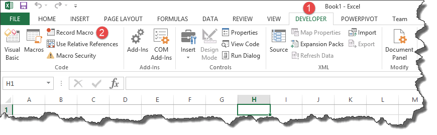
You will get the following dialogue window

- Enter ImportBankReceipts as the macro name.
- Step two will be there by default
- Enter the description as shown in the above diagram
- Click on “OK” tab
Step 6) Perform Macro Operations/Steps you want to record
- Put the cursor in cell A1
- Click on the DATA tab
- Click on From Text button on the Get External data ribbon bar
You will get the following dialogue window

- Go to the local drive where you have stored the CSV file
- Select the CSV file
- Click on Import button
You will get the following wizard

Click on Next button after following the above steps

Follow the above steps and click on next button

- Click on Finish button
- Your workbook should now look as follows

Step 7) Format the Data
Make the columns bold, add the grand total and use the SUM function to get the total amount.

Step  Stop Recording Macro
Now that we have finished our routine work, we can click on stop recording macro button as shown in the image below

Step 9) Replay the Macro
Before we save our work book, we will need to delete the imported data. We will do this to create a template that we will be copying every time we have new receipts and want to run the ImportBankReceipts macro.
- Highlight all the imported data
- Right click on the highlighted data
- Click on Delete
- Click on save as button
- Save the workbook in a macro enabled format as shown below

- Make a copy of the newly saved template
- Open it
- Click on DEVELOPER tab
- Click on Macros button
You will get the following dialogue window

- Select ImportBankReceipts
- Highlights the description of your macro
- Click on Run button
You will get the following data

Congratulations, you just created your first macro in Excel.
Summary
Macros simplify our work lives by automating most of the routine works that we do. Macros Excel are powered by Visual Basic for Applications.