
Excel for Microsoft 365 Excel for Microsoft 365 for Mac Excel for the web Excel 2021 Excel 2021 for Mac Excel 2019 Excel 2019 for Mac Excel 2016 Excel 2016 for Mac Excel 2013 Excel 2010 Excel 2007 Excel for Mac 2011 Excel Starter 2010 More…Less
Use Excel’s DATE function when you need to take three separate values and combine them to form a date.
The DATE function returns the sequential serial number that represents a particular date.
Syntax: DATE(year,month,day)
The DATE function syntax has the following arguments:
-
Year Required. The value of the year argument can include one to four digits. Excel interprets the year argument according to the date system your computer is using. By default, Microsoft Excel for Windows uses the 1900 date system, which means the first date is January 1, 1900.
Tip: Use four digits for the year argument to prevent unwanted results. For example, «07» could mean «1907» or «2007.» Four digit years prevent confusion.
-
If year is between 0 (zero) and 1899 (inclusive), Excel adds that value to 1900 to calculate the year. For example, DATE(108,1,2) returns January 2, 2008 (1900+108).
-
If year is between 1900 and 9999 (inclusive), Excel uses that value as the year. For example, DATE(2008,1,2) returns January 2, 2008.
-
If year is less than 0 or is 10000 or greater, Excel returns the #NUM! error value.
-
-
Month Required. A positive or negative integer representing the month of the year from 1 to 12 (January to December).
-
If month is greater than 12, month adds that number of months to the first month in the year specified. For example, DATE(2008,14,2) returns the serial number representing February 2, 2009.
-
If month is less than 1, month subtracts the magnitude of that number of months, plus 1, from the first month in the year specified. For example, DATE(2008,-3,2) returns the serial number representing September 2, 2007.
-
-
Day Required. A positive or negative integer representing the day of the month from 1 to 31.
-
If day is greater than the number of days in the month specified, day adds that number of days to the first day in the month. For example, DATE(2008,1,35) returns the serial number representing February 4, 2008.
-
If day is less than 1, day subtracts the magnitude that number of days, plus one, from the first day of the month specified. For example, DATE(2008,1,-15) returns the serial number representing December 16, 2007.
-
Note: Excel stores dates as sequential serial numbers so that they can be used in calculations. January 1, 1900 is serial number 1, and January 1, 2008 is serial number 39448 because it is 39,447 days after January 1, 1900. You will need to change the number format (Format Cells) in order to display a proper date.
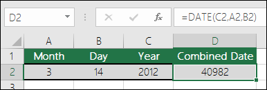
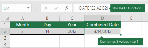
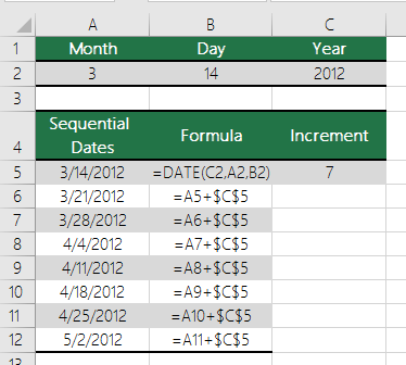
Syntax: DATE(year,month,day)
For example: =DATE(C2,A2,B2) combines the year from cell C2, the month from cell A2, and the day from cell B2 and puts them into one cell as a date. The example below shows the final result in cell D2.
Need to insert dates without a formula? No problem. You can insert the current date and time in a cell, or you can insert a date that gets updated. You can also fill data automatically in worksheet cells.
-
Right-click the cell(s) you want to change. On a Mac, Ctrl-click the cells.
-
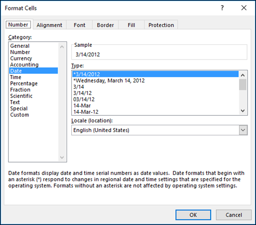
On the Home tab click Format > Format Cells or press Ctrl+1 (Command+1 on a Mac).
-
3. Choose the Locale (location) and Date format you want.
-
For more information on formatting dates, see Format a date the way you want.

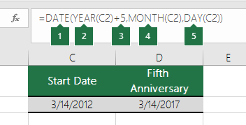
You can use the DATE function to create a date that is based on another cell’s date. For example, you can use the YEAR, MONTH, and DAY functions to create an anniversary date that’s based on another cell. Let’s say an employee’s first day at work is 10/1/2016; the DATE function can be used to establish his fifth year anniversary date:
-
The DATE function creates a date.
=DATE(YEAR(C2)+5,MONTH(C2),DAY(C2))
-
The YEAR function looks at cell C2 and extracts «2012».
-
Then, «+5» adds 5 years, and establishes «2017» as the anniversary year in cell D2.
-
The MONTH function extracts the «3» from C2. This establishes «3» as the month in cell D2.
-
The DAY function extracts «14» from C2. This establishes «14» as the day in cell D2.
If you open a file that came from another program, Excel will try to recognize dates within the data. But sometimes the dates aren’t recognizable. This is may be because the numbers don’t resemble a typical date, or because the data is formatted as text. If this is the case, you can use the DATE function to convert the information into dates. For example, in the following illustration, cell C2 contains a date that is in the format: YYYYMMDD. It is also formatted as text. To convert it into a date, the DATE function was used in conjunction with the LEFT, MID, and RIGHT functions.

-
The DATE function creates a date.
=DATE(LEFT(C2,4),MID(C2,5,2),RIGHT(C2,2))
-
The LEFT function looks at cell C2 and takes the first 4 characters from the left. This establishes “2014” as the year of the converted date in cell D2.
-
The MID function looks at cell C2. It starts at the 5th character, and then takes 2 characters to the right. This establishes “03” as the month of the converted date in cell D2. Because the formatting of D2 set to Date, the “0” isn’t included in the final result.
-
The RIGHT function looks at cell C2 and takes the first 2 characters starting from the very right and moving left. This establishes “14” as the day of the date in D2.
To increase or decrease a date by a certain number of days, simply add or subtract the number of days to the value or cell reference containing the date.
In the example below, cell A5 contains the date that we want to increase and decrease by 7 days (the value in C5).
See Also
Add or subtract dates
Insert the current date and time in a cell
Fill data automatically in worksheet cells
YEAR function
MONTH function
DAY function
TODAY function
DATEVALUE function
Date and time functions (reference)
All Excel functions (by category)
All Excel functions (alphabetical)
Need more help?
Want more options?
Explore subscription benefits, browse training courses, learn how to secure your device, and more.
Communities help you ask and answer questions, give feedback, and hear from experts with rich knowledge.
Date Range in Excel Formula
We need to perform different operations like addition or subtraction on date values with Excel. By setting date ranges in Excel, we can perform calculations on these dates. For setting date ranges in Excel, we can first format the cells that have a start and end date as ‘Date’ and then use the operators: ‘+’ or ‘-‘to determine the end date or range duration.
For example, suppose we have two dates in cells A2 and B2. To create a date range, we may use the following formula with the TEXT function:
=TEXT(A2,”mm/dd”)&” – “&TEXT(B2,”mm/dd”)
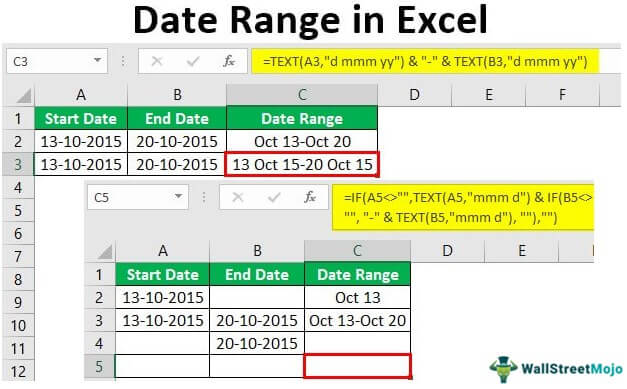
Table of contents
- Date Range in Excel Formula
- Examples of Date Range in Excel
- Example #1 – Basic Date Ranges
- Example #2 – Creating Date Sequence
- Example #3
- Example #4
- Things to Remember
- Recommended Articles
- Examples of Date Range in Excel
Examples of Date Range in Excel
You can download this Date Range Excel Template here – Date Range Excel Template
Example #1 – Basic Date Ranges
Let us see how adding a number to a date can create a date range.
Suppose we have a start date in cell A2.
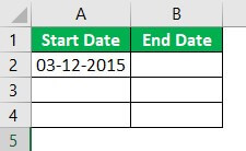
If we add a number, say 5, to it, we can build a date range.
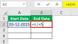
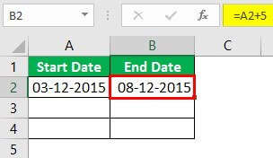
When we select cell A3 and type “=B2 + 1.”
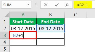
Then, we need to copy cell B2 and paste it into cell B3; the relative cell referenceCell reference in excel is referring the other cells to a cell to use its values or properties. For instance, if we have data in cell A2 and want to use that in cell A1, use =A2 in cell A1, and this will copy the A2 value in A1.read more would change as follows:
So we can see that multiple date ranges can be built this way.
Example #2 – Creating Date Sequence
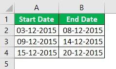
With Excel, we can easily create several sequences. Now we know that dates are some numbers in Excel. So we can use the same method to generate date ranges. So to create date ranges that have the same range or gap, but the dates change as we go down, we can follow the below steps:
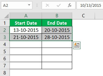
- We must first type a start date and end date in a minimum of two rows.
- Then, select the ranges and drag them down below the row where we require the dates ranges.
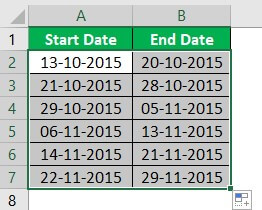
So we can see that using the date ranges in the first two rows as a template, Excel automatically creates date ranges for the subsequent rows.
Example #3
Now, suppose we have two dates in two cells, and we wish to display them concatenated as a date range in a single cell. For doing this, we can use a formula based on the ‘TEXT’ function can be used. The general syntax for this formula is as follows:
= TEXT(date1,”format”) & ” – ” & TEXT(date2,”format”)
Case 1:
This function receives two date values as numeric and concatenates these two dates in the form of a date range according to a custom date format (“mmm d” in this case):
Date Range =TEXT(A2,”mmm d”) & “-” & TEXT(B2,”mmm d”)
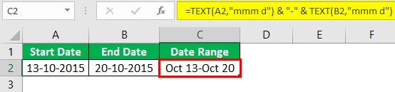
So we can see in the above screenshot that we have applied the formula in cell C2. The TEXT function receives the dates stored in cells A2 and B2. The ampersand ‘&’ operator is used to concatenate the two dates as a date range in a custom format, specified as “mmm d” in this case, in a single cell, and the two dates are joined with a hyphen ‘-‘ in the resultant date range which is determined in cell C2.
Case 2:
In this example, we wish to combine the two dates as a date range in a single cell with a different format, say “d mmm yy.” So the formula for a date range, in this case, would be as follows:
Date Range =TEXT(A3,”d mmm yy”) & “-” & TEXT(B3,”d mmm yy”)
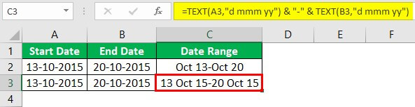
So we can see in the above screenshot that the TEXT function receives the dates stored in cells A3 and B3, and the ampersand ‘&’ operator is used to concatenate the two dates as a date range in a custom format, specified as “d mmm yy” in this case, in a single cell. Then, finally, the two dates are joined with a hyphen ‘-‘in the resultant date range determined in cell C3.
Example #4
Now let us see what happens if the start date or end date is missing. For example, suppose the end date is missing as follows:
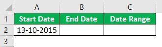
The formula based on the TEXT function that we have used above would not work correctly if the end date is missing. As the hyphen in the formula would anyhow be appended to the start date, i.e., along with the start date, we would also see a hyphen displayed in the date range. In contrast, we would only wish to see the start date as the date range if the end date is missing.
So, in this case, we can have the formula by wrapping the concatenation and the second TEXT function inside an IF clause as follows:
Date Range =TEXT(A2,”mmm d”) & IF(B2<> “”, “-” & TEXT(B2,”mmm d”), “”)
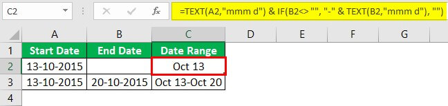
So we can see that the above formula creates a full date range using both the dates when both are present. However, it displays only the start date in the specified format if the end date is missing. It is done with the help of an IF clause.
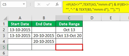
Now in case both the dates are missing, we could use a nested IF statement in excelIn Excel, nested if function means using another logical or conditional function with the if function to test multiple conditions. For example, if there are two conditions to be tested, we can use the logical functions AND or OR depending on the situation, or we can use the other conditional functions to test even more ifs inside a single if.read more, (i.e., one IF inside another IF statement) as follows:
Date Range =IF(A4<>””,TEXT(A4,”mmm d”) & IF(B4<> “”, “-” & TEXT(B4,”mmm d”), “”),””)

So we can see that the above formula returns an empty string if the start date is missing.
If both the dates are missing, an empty string is also returned.
Things to Remember
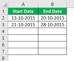
- We can even create a list of sequential dates using the ‘Fill Handle’ command. We can select the cell having a start date and then drag it to the range of cells where we wish to fill. Next, click on the “Home” tab -> “Editing” ->”Fill Series” and then choose a date unit we want to use.
- If we wish to calculate the duration or number of days between two dates, we can subtract the two dates using the ‘-‘operator, and we will get the desired result.

Note: The format of cells: A2 and B2 is ‘Date,’ whereas that of cell C2 is ‘General’ as it calculates the number of days.
Recommended Articles
This article has been a guide to Date Range in Excel. Here, we discuss formulas to create date ranges in Excel in different ways and a downloadable Excel template. You may learn more about Excel from the following articles: –
- DATE Excel Function
- EDATE Excel Function
- Subtract Date In Excel
- Compare Dates in Excel
In Microsoft Excel, the date can be inserted in a variety of ways, including using a built-in function formula or manually entering the date, such as 22/03/2021, 22-Mar-21, 22-Mar, or March 22, 2021. These date functions are typically used for cash flows in accounting and financial analysis.
In Excel, there is a built-in function called TODAY() that will insert the exact today’s date and will give the updated date whenever the workbook is opened. The NOW() built-in function can also be used to insert the current date and time, and this function will be kept up to date if we open the workbook multiple times.
Inserting the date:
In the Formula tab, the built-in TODAY is categorized under the DATE/TIME function.
Alternate to insert the date in Excel the below keyboard shortcut can be used:
CTRL+;
It will insert the current date.
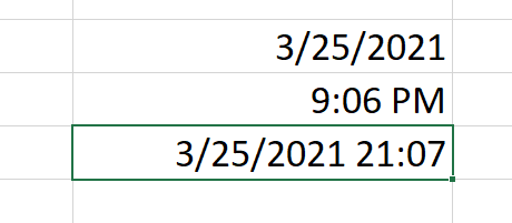
To insert the current date and time we can use the following shortcut keys:
CTRL+; <space key> CTRL+SHIFT+;
It returns the current date and time to us.
1. Inserting specific date in Excel:
We have to use DATE() to insert a specific valid date in Excel. We can notice in the above function that the DATE requests to provide Year, Month, Day values. If we provide the details, the default date will be shown as below:
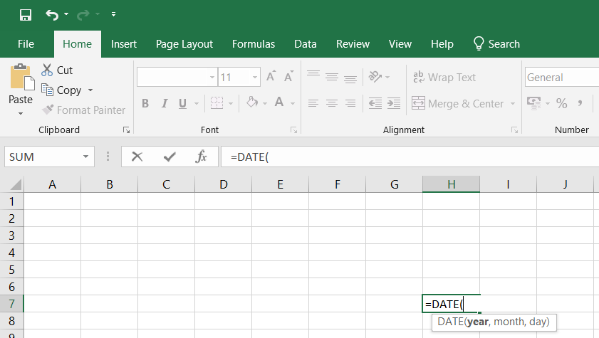
Image 1.1
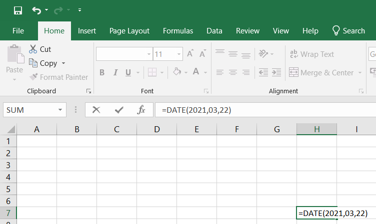
Image 1.2
2. Inserting static date and time:
A static value in a sheet does not change if the sheet is recalculated or opened. To do so follow the below steps:
Step 1: Select the cell in which the current date or time will be inserted on a table.
Step 2: Do one of the next:
- Press Ctrl+;(semi-colon) to insert your current date.
- Press the Ctrl+Shift+;(semi-colon) to insert the current time.
- Press Ctrl+;(semi-column) to insert the current date and time then press Space, and press Ctrl+Shift+; (semi-colon).
Static date and time
3. Inserting a date in Excel via a drop-down calendar:
It may be a good idea to include a down calendar in your worksheet if you set up a table for other users and want to make sure that the dates enter correctly. You can fill in the dates with a mouse click and be 100% confident that all dates are entered in a suitable format. You can use Microsoft Date Picker control when you use a 32-bit version of Excel. Microsoft Date Picker Control will not work when you are using a 64-bit Excel 2016, Excel 2013 version.
4. Inserting an automatically updatable today’s date and current time:
If you want to keep your Excel date up-to-date today, use one of the following Excel date functions:
=TODAY() -> inserts in a cell the current date.
=NOW() -> inserts in a cell the current and current date.
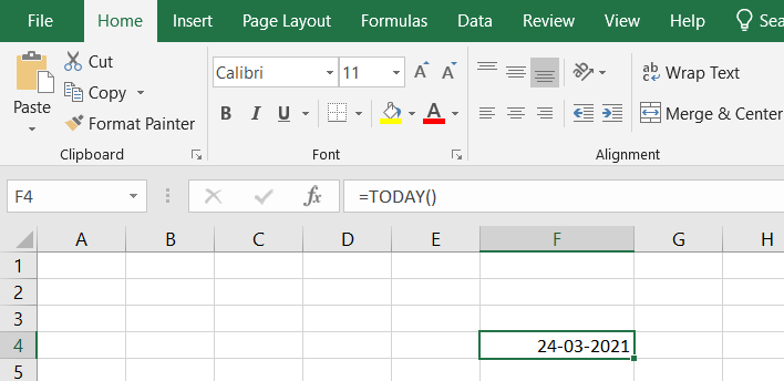
=TODAY example
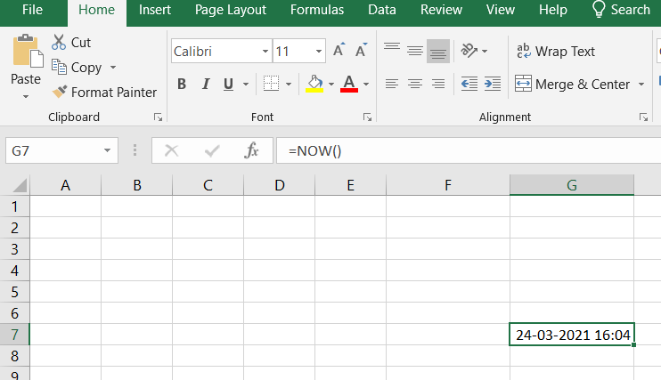
=NOW example
Please remember that when using the Excel date functions:
- The date and the time returned will not be refreshed on an ongoing basis, but only when the chain is reopened or re-calculated.
- The functions take the current system clock date and time.
5. Auto-populate dates in Excel
To autofill a series of dates in which one day is incremented, you can use the Excel AutoFill function. It is a common way to automatically fill a column or row. To do so follow the below steps:
- Enter the original date in the first cell.
- Click the first date on your cell and then drag the fill handle to or from the cells you want Excel to add dates.
Autofill weekdays, months, or years:
There are two ways of automatically adding weekdays, months, or years to the selected range of cells. To so follow the below steps:
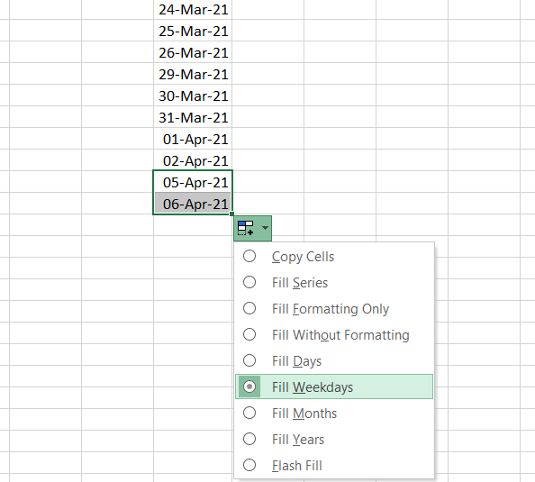
- You can use the above-mentioned Excel AutoFill options. Click the AutoFill Options icon and choose the option you want when the range is populated by sequential dates.
- Another way to enter your first date will be to right-click the fill handle and drag and release the fill handle through the cells you automatically want to fill with dates. Excel displays a context menu and selects the appropriate option.
Auto-populate dates
-
1
Type the desired date into a cell. Double-click the cell in which you want to type the date, and then enter the date using any recognizable date format. You can enter the date in a variety of different formats.[1]
- Using January 3 as an example, some recognizable formats are «Jan 03,» «January 3», «1/3,» and «01-3.»
-
2
Press the ↵ Enter key. As long as Excel recognizes the date format, it will re-format the cell as a date, which is usually mm/dd/yyyy or dd/mm/yyyy, depending on your locale.
- If the text automatically aligned to the right, then Excel recognized it as a date and re-formatted it.
- If the text stayed aligned to the left, Excel is treating the input as text rather than a date. This could be because it cannot recognize your input as a date, or because that cell’s format is set to something besides a date.
Advertisement
-
3
Right-click the date cell and select Format Cells. A new window will pop up.
-
4
Click the Number tab. It’s the first tab.
-
5
Select Date in the «Category» panel. A variety of date formats will appear on the right side of the window.
-
6
Select your desired date format under «Type.» This reformats the selected cell to display in this format.
- You can also change your locale to access date formats used in your location.
-
7
Click OK. The selected cell(s) will now display dates in the selected format.


Advertisement

-
1
Click the cell in which you want today’s date to appear. This can be in an existing formula, or in a new cell.
-
2
Type an equal sign = followed by the formula TODAY(). If you wish to retrieve the current time as well, use NOW() instead of TODAY().[2]
-
3
Hit ↵ Enter. Excel will return today’s date as the cell value. This is a dynamic date, meaning it will change depending on when you are viewing the sheet.
- Use the shortcuts Ctrl + ; and Ctrl + Shift + ; instead to set a cell’s value to today’s date and time respectively as a static value. These values will not update, and act as a timestamp.


Advertisement
-
1
Click the cell in which you want to type the date.
-
2
Type an equal sign = followed by the date formula DATE(year, month, day). Year, month, and day should be numerical inputs.
-
3
Hit ↵ Enter. Excel will return the default date format, which is usually mm/dd/yyyy or dd/mm/yyyy depending on your locale.
-
4
Expand on the formula if required. You can set formulas for the year, month, and day values. Or, you can use the DATE function within other formulas.
- For instance, DATE(2010,MONTH(TODAY()),DAY(TODAY())) sets the cell’s value as today’s month and day in 2010. The formula DATE(2020,1,1)-10 sets the value to 10 days before 1/1/2020.


Advertisement
-
1
Type the desired date into a cell. Double-click the cell in which you want to type the date, and then enter the date using any recognizable date format. You can enter the date in a variety of different formats.
- Using January 3 as an example, some recognizable formats are «Jan 03,» «January 3», «1/3,» and «01-3.»
-
2
Hit ↵ Enter. Excel will re-format the cell and align the text to the right if it has recognized it as a date.
-
3
Select all the cells you wish to fill with dates. Include the cell in which you just entered the date. To select, drag your mouse over all the cells, select an entire column or row, or hold Ctrl (PC) or ⌘ Cmd (Mac) while clicking each cell.
-
4
Click Fill on the Home tab. It’s at the top of Excel in the «Editing» section and looks like a white box with a blue down arrow.
-
5
Click Series…. It is near the bottom.
-
6
Select a «Date unit.» Excel will use this to fill the blank cells based on this setting.
- For instance, if you select «Weekday,» all the blank cells will populate with the weekdays following the initial input date.
-
7
Click OK. Make sure the are dates filled in correctly.


Advertisement
Ask a Question
200 characters left
Include your email address to get a message when this question is answered.
Submit
Advertisement
-
Set a custom date format in Excel by right-clicking a cell, clicking Format Cells, and selecting «Custom» as the category in the Number tab. Review the available date options. Create your own by typing the format code using an existing code.
Advertisement
References
About This Article
Article SummaryX
1. Click on a cell.
2. Type in a date.
3. Hit Enter.
4. Review the date format. Change by right-clicking and selecting Format Cells.
Did this summary help you?
Thanks to all authors for creating a page that has been read 12,928 times.