
Excel для Microsoft 365 Excel для Microsoft 365 для Mac Excel 2021 Excel 2021 для Mac Excel 2019 Excel 2019 для Mac Excel 2016 Excel 2016 для Mac Excel 2013 Excel 2010 Excel 2007 Excel для Mac 2011 Еще…Меньше
С помощью средств анализа «что если» в Excel вы можете экспериментировать с различными наборами значений в одной или нескольких формулах, чтобы изучить все возможные результаты.
Например, можно выполнить анализ «что если» для формирования двух бюджетов с разными предполагаемыми уровнями дохода. Или можно указать нужный результат формулы, а затем определить, какие наборы значений позволят его получить. В Excel предлагается несколько средств для выполнения разных типов анализа.
Обратите внимание на то, что в этой статье приведен только обзор инструментов. Подробные сведения о каждом из них можно найти по ссылкам ниже.
Анализ «что если» — это процесс изменения значений в ячейках, который позволяет увидеть, как эти изменения влияют на результаты формул на листе.
В Excel предлагаются средства анализа «что если» трех типов: сценарии, таблицы данных и подбор параметров. В сценариях и таблицах данных берутся наборы входных значений и определяются возможные результаты. Таблицы данных работают только с одной или двумя переменными, но могут принимать множество различных значений для них. Сценарий может содержать несколько переменных, но допускает не более 32 значений. Подбор параметров отличается от сценариев и таблиц данных: при его использовании берется результат и определяются возможные входные значения для его получения.
Помимо этих трех средств можно установить надстройки для выполнения анализа «что если», например надстройку Поиск решения. Эта надстройка похожа на подбор параметров, но позволяет использовать больше переменных. Вы также можете создавать прогнозы, используя маркер заполнения и различные команды, встроенные в Excel.
Для более сложных моделей можно использовать надстройку Пакет анализа.
Сценарий
— это набор значений, которые сохраняются в Excel и могут автоматически подставляться в ячейки на листе. Вы можете создавать и сохранять различные группы значений на листе, а затем переключиться на любой из этих новых сценариев, чтобы просмотреть другие результаты.
Предположим, у вас есть два сценария бюджета: для худшего и лучшего случаев. Вы можете с помощью диспетчера сценариев создать оба сценария на одном листе, а затем переключаться между ними. Для каждого сценария вы указываете изменяемые ячейки и значения, которые нужно использовать. При переключении между сценариями результат в ячейках изменяется, отражая различные значения изменяемых ячеек.
1. Изменяемые ячейки
2. Ячейка результата
1. Изменяемые ячейки
2. Ячейка результата
Если у нескольких человек есть конкретные данные в отдельных книгах, которые вы хотите использовать в сценариях, вы можете собрать эти книги и объединить их сценарии.
После создания или сбора всех нужных сценариев вы можете создать сводный отчет по сценариям, в который включаются данные из этих сценариев. В отчете по сценариям все данные отображаются в одной таблице на новом листе.
Примечание: В отчетах по сценариям автоматический пересчет не выполняется. Изменения значений в сценарии не будут отражается в уже существующем сводном отчете. Вам потребуется создать новый сводный отчет.
Если вы знаете нужный результат формулы, но не знаете, какое входные значения требуется для получения этого результата, используйте функцию «Поиск окна». Предположим, что вам нужно занять денег. Вы знаете, сколько вам нужно, на какой срок и сколько вы сможете выплачивать каждый месяц. С помощью средства подбора параметров вы можете определить, какая процентная ставка вам подойдет.
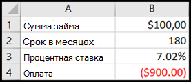
Ячейки B1, B2 и B3 — это значения для суммы займа, длины срока и процентной ставки.
Ячейка B4 отображает результат формулы =PMT(B3/12;B2;B1).
Примечание: В средстве поиска окна можно ввести только одно значение переменной. Если вы хотите определить несколько входных значений, например сумму займа и сумму ежемесячного платежа по кредиту, используйте надстройка «Надстройка «Найти решение». Дополнительные сведения о надстройки «Решение» см. в разделе Подготовка прогнозов и расширенных бизнес-моделей ипо ссылкам в разделе См. также.
Если у вас есть формула с одной или двумя переменными либо несколько формул, в которых используется одна общая переменная, вы можете просмотреть все результаты в одной таблице данных. С помощью таблиц данных можно легко и быстро проверить несколько возможностей. Поскольку используются всего одна или две переменные, результат можно без труда прочитать или опубликовать в табличной форме. Если для книги включен автоматический пересчет, данные в таблицах данных сразу же пересчитываются, и вы всегда видите свежие данные.
Ячейка B3 содержит входные значения.
Ячейки C3, C4 и C5 являются значениями, Excel заменяются на основе значения, введенного в ячейку B3.
В таблицу данных нельзя помещать больше двух переменных. Для анализа большего количества переменных используйте сценарии. Несмотря на то что переменных не может быть больше двух, можно использовать сколько угодно различных значений переменных. В сценарии можно использовать не более 32 различных значений, зато вы можете создать сколько угодно сценариев.
При подготовке прогнозов вы можете использовать Excel для автоматической генерации будущих значений на базе существующих данных или для автоматического вычисления экстраполированных значений на основе арифметической или геометрической прогрессии.
Вы можете заполнить ряд значений, которые соответствуют простому линейному или экспоненциальному тренду роста, с помощью ручки заполнения или команды Ряд. Для расширения сложных и нелинейных данных можно использовать функции или средство регрессионного анализа надстройки «Надстройка анализа».
В средстве подбора параметров можно использовать только одну переменную, а с помощью надстройки Поиск решения вы можете создать обратную проекцию для большего количества переменных. Надстройка «Поиск решения» помогает найти оптимальное значение для формулы в одной ячейке листа, которая называется целевой.
Над решением работает группа ячеек, связанных с формулой в целевой ячейке. «Решение» изменяет значения изменяемых ячеек, которые вы указываете (регулируемые ячейки), чтобы получить результат, который вы указываете из формулы целевой ячейки. Ограничения можно применять для ограничения значений, которые можно использовать в модели, а ограничения могут ссылаться на другие ячейки, влияющие на формулу целевой ячейки.
Дополнительные сведения
Вы всегда можете задать вопрос специалисту Excel Tech Community или попросить помощи в сообществе Answers community.
См. также
Сценарии
Подбор параметров
Таблицы данных
Использование «Решения» для бюджетов с использованием средств на счете вех
Использование «Решение» для определения оптимального сочетания продуктов
Постановка и решение задачи с помощью надстройки «Поиск решения»
Надстройка «Надстройка анализа»
Полные сведения о формулах в Excel
Рекомендации, позволяющие избежать появления неработающих формул
Обнаружение ошибок в формулах
Сочетания клавиш в Excel
Функции Excel (по алфавиту)
Функции Excel (по категориям)
Нужна дополнительная помощь?
Excel for Microsoft 365 Excel for Microsoft 365 for Mac Excel 2021 Excel 2021 for Mac Excel 2019 Excel 2019 for Mac Excel 2016 Excel 2016 for Mac Excel 2013 Excel 2010 Excel 2007 Excel for Mac 2011 More…Less
By using What-If Analysis tools in Excel, you can use several different sets of values in one or more formulas to explore all the various results.
For example, you can do What-If Analysis to build two budgets that each assumes a certain level of revenue. Or, you can specify a result that you want a formula to produce, and then determine what sets of values will produce that result. Excel provides several different tools to help you perform the type of analysis that fits your needs.
Note that this is just an overview of those tools. There are links to help topics for each one specifically.
What-If Analysis is the process of changing the values in cells to see how those changes will affect the outcome of formulas on the worksheet.
Three kinds of What-If Analysis tools come with Excel: Scenarios, Goal Seek, and Data Tables. Scenarios and Data tables take sets of input values and determine possible results. A Data Table works with only one or two variables, but it can accept many different values for those variables. A Scenario can have multiple variables, but it can only accommodate up to 32 values. Goal Seek works differently from Scenarios and Data Tables in that it takes a result and determines possible input values that produce that result.
In addition to these three tools, you can install add-ins that help you perform What-If Analysis, such as the Solver add-in. The Solver add-in is similar to Goal Seek, but it can accommodate more variables. You can also create forecasts by using the fill handle and various commands that are built into Excel.
For more advanced models, you can use the Analysis ToolPak add-in.
A Scenario is a set of values that Excel saves and can substitute automatically in cells on a worksheet. You can create and save different groups of values on a worksheet and then switch to any of these new scenarios to view different results.
For example, suppose you have two budget scenarios: a worst case and a best case. You can use the Scenario Manager to create both scenarios on the same worksheet, and then switch between them. For each scenario, you specify the cells that change and the values to use for that scenario. When you switch between scenarios, the result cell changes to reflect the different changing cell values.
1. Changing cells
2. Result cell
1. Changing cells
2. Result cell
If several people have specific information in separate workbooks that you want to use in scenarios, you can collect those workbooks and merge their scenarios.
After you have created or gathered all the scenarios that you need, you can create a Scenario Summary Report that incorporates information from those scenarios. A scenario report displays all the scenario information in one table on a new worksheet.
Note: Scenario reports are not automatically recalculated. If you change the values of a scenario, those changes will not show up in an existing summary report. Instead, you must create a new summary report.
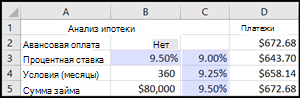
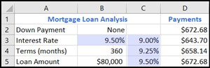
If you know the result that you want from a formula, but you’re not sure what input value the formula requires to get that result, you can use the Goal Seek feature. For example, suppose that you need to borrow some money. You know how much money you want, how long a period you want in which to pay off the loan, and how much you can afford to pay each month. You can use Goal Seek to determine what interest rate you must secure in order to meet your loan goal.

Cells B1, B2, and B3 are the values for the loan amount, term length, and interest rate.
Cell B4 displays the result of the formula =PMT(B3/12,B2,B1).
Note: Goal Seek works with only one variable input value. If you want to determine more than one input value, for example, the loan amount and the monthly payment amount for a loan, you should instead use the Solver add-in. For more information about the Solver add-in, see the section Prepare forecasts and advanced business models, and follow the links in the See Also section.
If you have a formula that uses one or two variables, or multiple formulas that all use one common variable, you can use a Data Table to see all the outcomes in one place. Using Data Tables makes it easy to examine a range of possibilities at a glance. Because you focus on only one or two variables, results are easy to read and share in tabular form. If automatic recalculation is enabled for the workbook, the data in Data Tables immediately recalculates; as a result, you always have fresh data.
Cell B3 contains the input value.
Cells C3, C4, and C5 are values Excel substitutes based on the value entered in B3.
A Data Table cannot accommodate more than two variables. If you want to analyze more than two variables, you can use Scenarios. Although it is limited to only one or two variables, a Data Table can use as many different variable values as you want. A Scenario can have a maximum of 32 different values, but you can create as many scenarios as you want.
If you want to prepare forecasts, you can use Excel to automatically generate future values that are based on existing data, or to automatically generate extrapolated values that are based on linear trend or growth trend calculations.
You can fill in a series of values that fit a simple linear trend or an exponential growth trend by using the fill handle or the Series command. To extend complex and nonlinear data, you can use worksheet functions or the regression analysis tool in the Analysis ToolPak Add-in.
Although Goal Seek can accommodate only one variable, you can project backward for more variables by using the Solver add-in. By using Solver, you can find an optimal value for a formula in one cell—called the target cell—on a worksheet.
Solver works with a group of cells that are related to the formula in the target cell. Solver adjusts the values in the changing cells that you specify—called the adjustable cells—to produce the result that you specify from the target cell formula. You can apply constraints to restrict the values that Solver can use in the model, and the constraints can refer to other cells that affect the target cell formula.
Need more help?
You can always ask an expert in the Excel Tech Community or get support in the Answers community.
See Also
Scenarios
Goal Seek
Data Tables
Using Solver for capital budgeting
Using Solver to determine the optimal product mix
Define and solve a problem by using Solver
Analysis ToolPak Add-in
Overview of formulas in Excel
How to avoid broken formulas
Detect errors in formulas
Keyboard shortcuts in Excel
Excel functions (alphabetical)
Excel functions (by category)
Need more help?
If you’ve ever experimented with different variables to see how your changes would affect the outcome of a situation, you’ve done a what if analysis.
Would you be able to sell more items if you had a sale this week? Or would you make more money by increasing the price instead? In the above scenarios, you want to know the degree to which each change affects the overall outcome. For this reason, a what if analysis is also known as a sensitivity analysis.
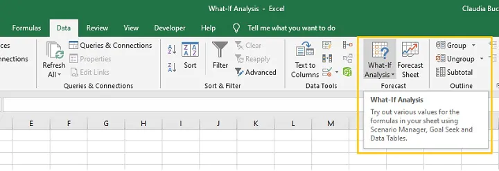
Most what if analyses are really mathematical calculations, and that is Excel’s specialty. To help you do a what if analysis, Excel uses commands from the Forecast command group on the Data tab to prepare simple forecasts or advanced business models.
Download your free Excel practice file
Use this free Excel file to practice what if analysis along with the tutorial.
Goal Seek
The simplest sensitivity analysis tool in Excel is Goal Seek. Assuming that you know the single outcome you would like to achieve, the Goal Seek feature in Excel allows you to arrive at that goal by mathematically adjusting a single variable within the equation.
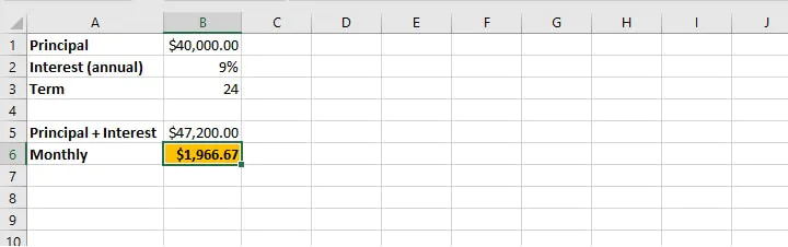
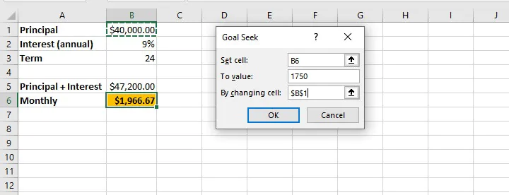
 To illustrate how it works, imagine that the bank is offering an interest rate of 9% per annum on personal loans with 24 months to repay, and that you would like to borrow $40,000.
Using the above information, the bank calculates that the amount borrowed plus interest over the loan period will be $47,200, as shown in cell B5. The amount to be paid each month is also calculated and shown in cell B6.
 By using the Goal Seek command, we can indicate a desired outcome and Excel will determine the adjustment we need to make to a single variable.
In the example above, cell B5 is dependent on the variables in cells B1, B2, and B3. Cell B6 is dependent on cells B3 and B5. Therefore, if we determine that the monthly repayment amount quoted is higher than desired, we can use Goal Seek to set the monthly amount to $1750. Excel can work backwards to change either cell B1, B2, or B3 to reach that goal.
Practically speaking, we may not have much control over the interest rate, so it is more likely that we have the option of adjusting the amount we borrow, or the repayment period.
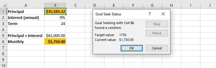
Our first inclination may be to find out how much we will be able to borrow if we pay $1750 per month and all other variables remain the same. Excel will change the principal (B1) based on the number we enter as the new value for cell B6.
 Assuming that the interest amount (9%) and loan period (24 months) remain the same, the new principal amount is calculated and displayed in cell B1 if a valid solution exists.
 Points to note:
- The cell chosen in the “Set cell” field must be a cell containing a formula.
- The cell chosen in the “By changing cell” field must be a cell containing a constant.
- Once “OK” is selected from the Goal Seek Status window, the values on the worksheet are adjusted and are only retrievable by selecting the ‘Undo’ command (Ctrl+Z Windows shortcut/Cmd+Z Mac shortcut).
Scenario Manager
Another what if analysis tool is the Scenario Manager. This option is somewhat more advanced than Goal Seek in that it allows the adjustment of multiple variables at the same time.
 Some other noticeable differences between Goal Seek and Scenario Manager are listed below:
- The Scenario Manager allows the creation of an unlimited number of possible scenarios by changing up to 32 variables at a time.
- Each scenario can be saved for comparative purposes.
- Scenarios may be named and edited, and a brief description provided.
- Only constant values should be changed within the Scenario Manager — cells with formulas should not be manually adjusted.
If we continue our bank loan example, we can determine our model’s sensitivity to change by adjusting any or all of the values in cell B1, B2, or B3.
Best practice
As a best practice, the original worksheet data should be saved as a scenario so that you can revert to it after all the experiments have been completed.
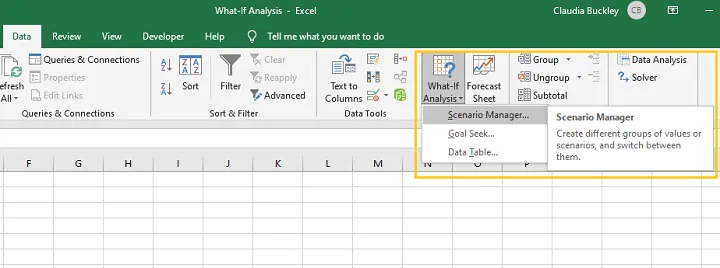
Step 1 — Click ‘What If Analysis’ from the Data tab and select Scenario Manager.
Step 2 — Click ‘Add’ from the Scenario Manager pop-up window.
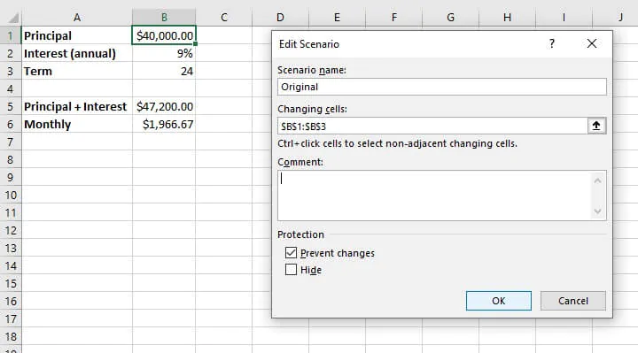
Step 3 — Name this scenario “Original” and enter the cell references of all cells with constant values that you may consider changing in other scenarios (maximum 32 cells). Click OK.
 Step 4 — For the “Original” scenario, do not adjust any values in the ‘Scenario Values’ window.
 Step 5 — Click ‘Add’ to create your first experimental scenario.
Creating experimental scenarios
When creating an experimental scenario, give the scenario a descriptive name from the ‘Add Scenario’ pop-up window. The changing cells will be the same as the ones referenced in your ‘Original’ scenario.
Even if you will not be adjusting all the values in those cells, it is highly recommended that they remain referenced in the ‘changing cells’ field. You may place additional details about the experimental scenario in the ‘Comment’ field (see below).
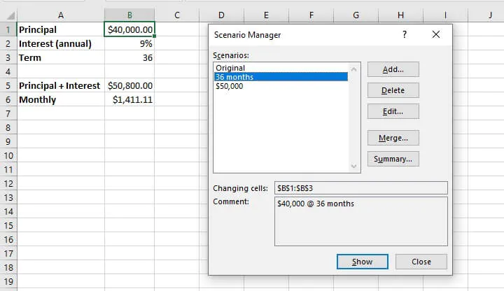
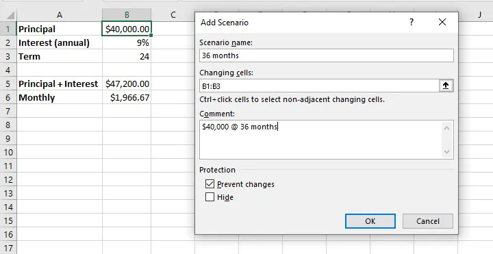 As illustrated above, our experimental scenario is given the name “36 months” and refers to cells B1 to B3 as changing cells. An additional comment indicates that this scenario is to determine the effect of borrowing $40,000 over a 36-month period.
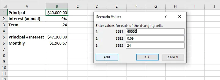
In the ‘Scenario Values’ window, each changing cell is displayed as a field where we can manipulate the constant value so as to affect the outcome of the dependent cells — in our case, cells B5 and B6. As described in our scenario name and comments, we only adjust cell B3 by changing the value to 36.
To add another scenario at this point, select ‘Add’. If not, click OK.
Adjust multiple variables
To experiment with adjusting multiple variables within one scenario, the steps are the same as above, with the exception that the desired changes would be made in the Scenario Values window.
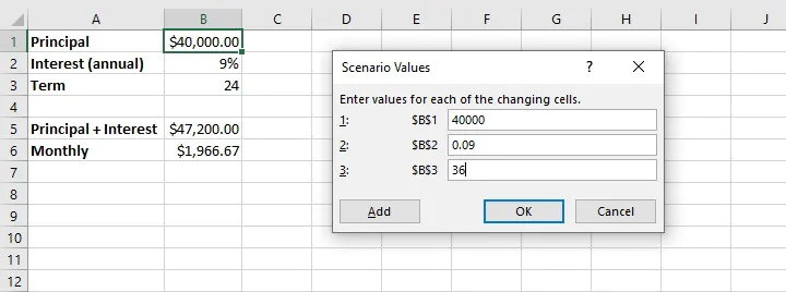
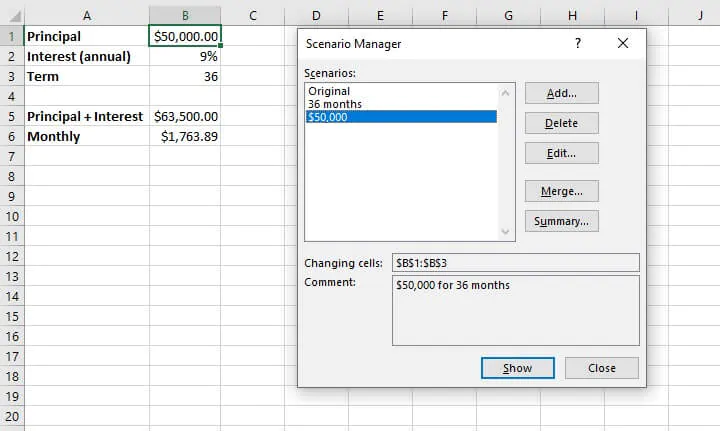
For example, to get Excel to perform a what if analysis on borrowing $50,000 over a 36-month period in the above situation at the same rate of interest, we would simply adjust the fields referencing those variables after creating a new scenario. Excel’s Scenario Manager can handle an unlimited number of scenarios created in this same way.
A list of created scenarios can be viewed by clicking OK from the Scenario Values window, or by selecting Scenario Manager from the What If Analysis dropdown menu.
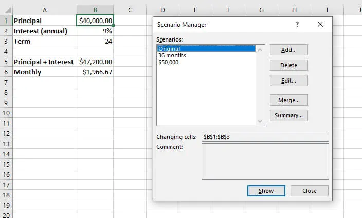 To see the outcome of each adjustment on the output cell(s), either double click on a scenario name, or highlight a name and click Show.
Scenario summary
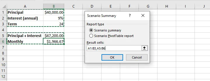
Scenarios that have been created may also be compared side by side with the creation of a Scenario summary worksheet, which is generated by selecting ‘Summary’ from the Scenario Manager window.
There are two report types available — Scenario summary and Scenario PivotTable report. Result cells are the cells that will be displayed in the summary. Ideally, these should include all cells which were adjusted as well as result cells. It’s also a good idea to select cells that contain header names so that these are clearly displayed in the summary.
 Choosing the ‘Scenario summary’ option will create a new sheet within the workbook that displays each scenario in columnar format. Changing Cells are highlighted in gray, and Result Cells are displayed under Changing Cells.
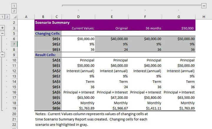 Note that if named ranges were created for Changing or Result Cells, range names will be displayed instead of cell references.
Selecting the Scenario PivotTable report type will create a pivot table report in a new worksheet. Learn more about pivot tables from our Resource Library.
Using data tables for what if analysis
The third what if analysis tool from the Forecast command group is the Data Table. Data tables allow the adjustment of only one or two variables within a dataset, but each variable can have an unlimited number of possible values. Data tables are designed for side-by-side comparisons in a way that makes them easier to read than scenarios, once they are set up correctly.
Data tables are under-utilized, but are not as scary as they may seem.
One-variable data tables
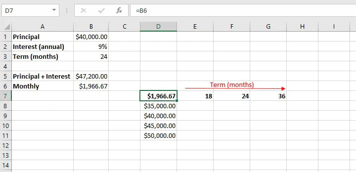
If the only variable to be considered in our loan example were the amount being borrowed, we could set up a one-variable data table.
Step 1 — make a list of all possible principal loan amounts. The list may be by column or row. In our example, we will enter a column list in the range D9 to D12.
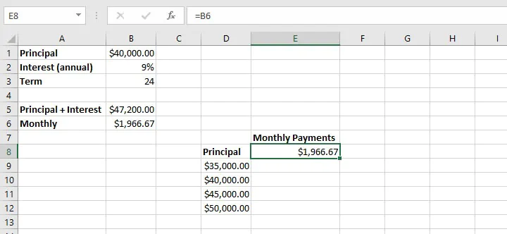
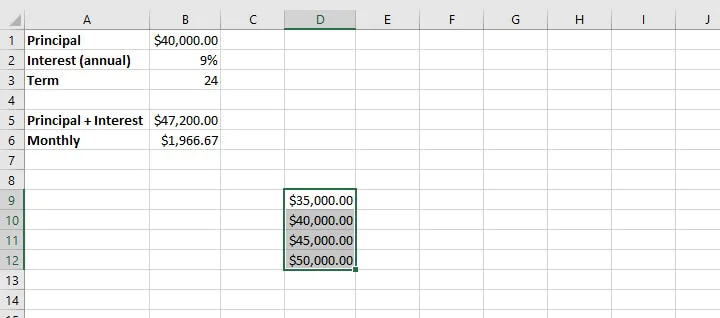 Step 2 — In an adjacent column, enter the formula which was used to arrive at the original outcome. In this case, we can simply type =B6 in cell E8. This links our new data table to the original variables.
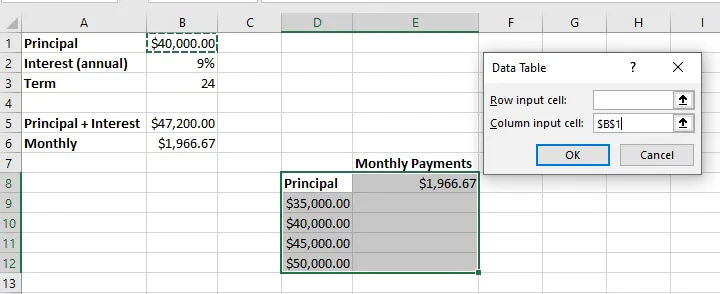
 Step 3 — Select the entire data table range, including the list of variable values, the formula, and blank cells.
Step 4 — From the What If Analysis dropdown menu, select Data Table.
Step 5 — In the column input cell field (since we entered our variables in column format), enter the cell reference that was used to calculate the result in the original dataset. In the above example, this would be cell B1 since this is the variable we have adjusted. No value is entered in the ‘Row input cell’ field in this instance since this is a one-variable data table.
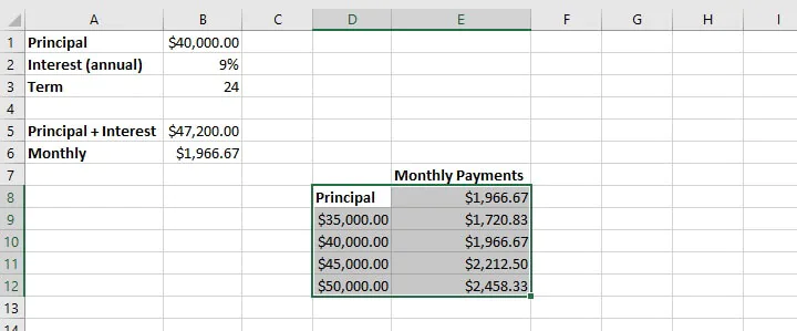
 Step 6 — Select OK. The result is a list of outcomes created by adjusting the one variable in cell B1, assuming that all other variables remain constant.
 To create a row-oriented data table, the variables would be listed horizontally, and the row input cell would be used in the Data Table window instead of the column input cell.
Two-variable data tables
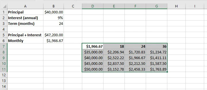
When creating a two-variable data table, one set of values is listed horizontally and the other set is listed vertically. In our example, we will add the loan period (term) as our second variable, displayed horizontally.
In this case, the formula which was used to arrive at the original outcome must be replicated above the vertical list of variables. As shown below, we type =B6 in cell D7. This links our new data table to the original variables.
 As before, highlight the entire data table range and select Data Table from the What If Analysis menu. The row input cell is the cell reference (B3) that corresponds to the horizontal variables from the original dataset, while the column input cell (B1) corresponds to the vertical variables.
When we select OK, Excel returns a matrix that can be used to compare the outcome of different changes to our original scenario. It may be necessary to adjust the output cells to the appropriate number format for your data type (in the case of the above example, currency).
Summary
Now that you’ve taken the time to demystify how to do a what if analysis in Excel by using these three main tools, why not experiment with using them in different settings — like budget management, profit margin percentages, project completion targets, and the like?
Once you get the hang of these, you’ll want to check out our resource center and take our Basic and Advanced Excel course to become a real pro!
Ready to become a certified Excel ninja?
Start learning for free with GoSkills courses
Start free trial
Excel’s What-If Analysis Scenario Manager helps you compare multiple data sets and decide based on data analysis.

Excel has many powerful tools, including the What-If Analysis, which helps you perform different types of mathematical calculations. It allows you to experiment with different formula parameters to explore the effects of variations in the result.
So, instead of dealing with complex mathematical calculations to get the answers you seek, you can simply use the What-If Analysis in Excel.
When Is What-If Analysis Used?
You should use the What-If Analysis if you would like to see how a change of value in your cells will affect the outcome of the formulas in your worksheet.
Excel provides different tools that will help you perform all sorts of analyses that fit your needs. So it all comes down to what you want.
For example, you can use the What-If Analysis if you want to build two budgets, both of which will require a certain level of revenue. With this tool, you could also determine what sets of values you need in order to produce a certain result.

There are three kinds of What-If Analysis tools that you have in Excel: Goal Seek, Scenarios, and Data Tables.
Goal Seek
When you create a function or a formula in Excel, you put different parts together to get appropriate results. However, Goal Seek works oppositely, as you get to start with the result you want.
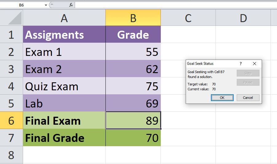
Goal Seek is most often used if you want to know the value that you need to get a certain result. For example, if you want to calculate the grade, you would need to get in school in order for you to pass the class.
A simple example would look like this. If you would like your final grade to have an average of 70 points, you first need to calculate your overall average, including the empty cell.
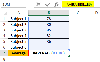
You can do that with this function:
<strong>=AVERAGE(B2:B6)</strong>
Once you know your average, you should go to Data > What-If Analysis > Goal Seek. Then calculate the Goal Seek using the information that you have. In this case, that would be:
If you want to learn more about it, you can check out our following guide on Goal Seek.
Scenarios
In Excel, Scenarios allow you to substitute values for multiple cells simultaneously (up to 32). You can create many Scenarios and compare them without having to change the values manually.
For example, if you have the worst and the best-case scenarios, you can use the Scenario Manager in Excel to create both of these scenarios.
In both scenarios, you need to specify the cells that change values, and the values that might be used for that scenario. You can find a good example of this on Microsoft’s website.
Data Tables
Unlike Goal Seek or Scenarios, this option allows you to see multiple results simultaneously. You can replace one or two variables in a formula with as many different values as you like and then see the results in a table.
This makes it easy to examine a range of possibilities with just one glance. However, a Data Table cannot accommodate more than 2 variables. If that is what you were hoping for, you should use Scenarios instead.

Visualize Your Data With What-If Analysis in Excel
If you use Excel frequently, you will discover many formulas and functions that make life easier. The What-If Analysis is just one of many examples that can simplify your most complex mathematical calculations.
With the What-If Analysis in Excel, you get to experiment with different answers to the same question, even if your data is incomplete. To get the most out of the What-If Analysis, you should be fairly comfortable with functions and formulas in Excel.
Содержание
- What-If Analysis
- Create Different Scenarios
- Scenario Summary
- Goal Seek
- IF function – nested formulas and avoiding pitfalls
- Remarks
- Examples
- Additional examples
- Did you know?
- Need more help?
- What-If Analysis in Excel
- What is a What-If Analysis in Excel?
- #1 Scenario Manager in What-If Analysis
- #2 Goal Seek in What-If Analysis
- #3 Data Table in What-If Analysis
- Things to Remember
- Recommended Articles
What-If Analysis
What-If Analysis in Excel allows you to try out different values (scenarios) for formulas. The following example helps you master what-if analysis quickly and easily.
Assume you own a book store and have 100 books in storage. You sell a certain % for the highest price of $50 and a certain % for the lower price of $20.
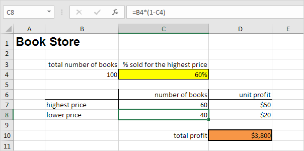
If you sell 60% for the highest price, cell D10 calculates a total profit of 60 * $50 + 40 * $20 = $3800.
Create Different Scenarios
But what if you sell 70% for the highest price? And what if you sell 80% for the highest price? Or 90%, or even 100%? Each different percentage is a different scenario. You can use the Scenario Manager to create these scenarios.
Note: You can simply type in a different percentage into cell C4 to see the corresponding result of a scenario in cell D10. However, what-if analysis enables you to easily compare the results of different scenarios. Read on.
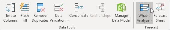
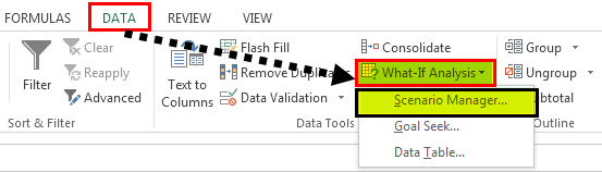
1. On the Data tab, in the Forecast group, click What-If Analysis.
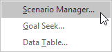
2. Click Scenario Manager.
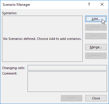
The Scenario Manager dialog box appears.
3. Add a scenario by clicking on Add.
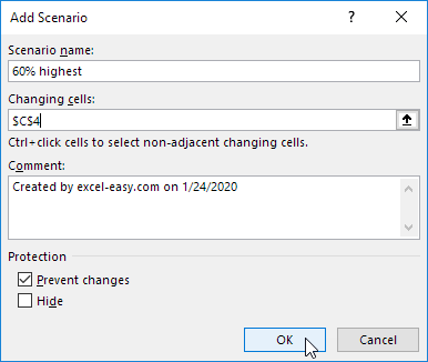
4. Type a name (60% highest), select cell C4 (% sold for the highest price) for the Changing cells and click on OK.
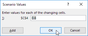
5. Enter the corresponding value 0.6 and click on OK again.
6. Next, add 4 other scenarios (70%, 80%, 90% and 100%).
Finally, your Scenario Manager should be consistent with the picture below:
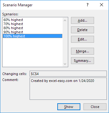
Note: to see the result of a scenario, select the scenario and click on the Show button. Excel will change the value of cell C4 accordingly for you to see the corresponding result on the sheet.
Scenario Summary
To easily compare the results of these scenarios, execute the following steps.
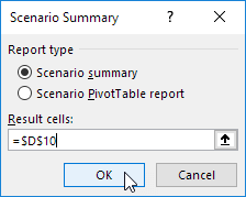
1. Click the Summary button in the Scenario Manager.
2. Next, select cell D10 (total profit) for the result cell and click on OK.
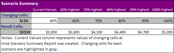
Conclusion: if you sell 70% for the highest price, you obtain a total profit of $4100, if you sell 80% for the highest price, you obtain a total profit of $4400, etc. That’s how easy what-if analysis in Excel can be.
Goal Seek
What if you want to know how many books you need to sell for the highest price, to obtain a total profit of exactly $4700? You can use Excel’s Goal Seek feature to find the answer.
1. On the Data tab, in the Forecast group, click What-If Analysis.
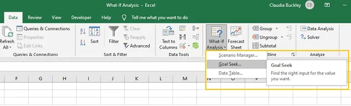
2. Click Goal Seek.
The Goal Seek dialog box appears.
3. Select cell D10.
4. Click in the ‘To value’ box and type 4700.
5. Click in the ‘By changing cell’ box and select cell C4.
Result. You need to sell 90% of the books for the highest price to obtain a total profit of exactly $4700.

Note: visit our page about Goal Seek for more examples and tips.
Источник
IF function – nested formulas and avoiding pitfalls
The IF function allows you to make a logical comparison between a value and what you expect by testing for a condition and returning a result if True or False.
=IF(Something is True, then do something, otherwise do something else)
So an IF statement can have two results. The first result is if your comparison is True, the second if your comparison is False.
IF statements are incredibly robust, and form the basis of many spreadsheet models, but they are also the root cause of many spreadsheet issues. Ideally, an IF statement should apply to minimal conditions, such as Male/Female, Yes/No/Maybe, to name a few, but sometimes you might need to evaluate more complex scenarios that require nesting* more than 3 IF functions together.
* “Nesting” refers to the practice of joining multiple functions together in one formula.
Use the IF function, one of the logical functions, to return one value if a condition is true and another value if it’s false.
IF(logical_test, value_if_true, [value_if_false])
The condition you want to test.
The value that you want returned if the result of logical_test is TRUE.
The value that you want returned if the result of logical_test is FALSE.
While Excel will allow you to nest up to 64 different IF functions, it’s not at all advisable to do so. Why?
Multiple IF statements require a great deal of thought to build correctly and make sure that their logic can calculate correctly through each condition all the way to the end. If you don’t nest your formula 100% accurately, then it might work 75% of the time, but return unexpected results 25% of the time. Unfortunately, the odds of you catching the 25% are slim.
Multiple IF statements can become incredibly difficult to maintain, especially when you come back some time later and try to figure out what you, or worse someone else, was trying to do.
If you find yourself with an IF statement that just seems to keep growing with no end in sight, it’s time to put down the mouse and rethink your strategy.
Let’s look at how to properly create a complex nested IF statement using multiple IFs, and when to recognize that it’s time to use another tool in your Excel arsenal.
Examples
Following is an example of a relatively standard nested IF statement to convert student test scores to their letter grade equivalent.
 97,»A+»,IF(B2>93,»A»,IF(B2>89,»A-«,IF(B2>87,»B+»,IF(B2>83,»B»,IF(B2>79,»B-«,IF(B2>77,»C+»,IF(B2>73,»C»,IF(B2>69,»C-«,IF(B2>57,»D+»,IF(B2>53,»D»,IF(B2>49,»D-«,»F»))))))))))))» loading=»lazy»>
This complex nested IF statement follows a straightforward logic:
If the Test Score (in cell D2) is greater than 89, then the student gets an A
If the Test Score is greater than 79, then the student gets a B
If the Test Score is greater than 69, then the student gets a C
If the Test Score is greater than 59, then the student gets a D
Otherwise the student gets an F
This particular example is relatively safe because it’s not likely that the correlation between test scores and letter grades will change, so it won’t require much maintenance. But here’s a thought – what if you need to segment the grades between A+, A and A- (and so on)? Now your four condition IF statement needs to be rewritten to have 12 conditions! Here’s what your formula would look like now:
It’s still functionally accurate and will work as expected, but it takes a long time to write and longer to test to make sure it does what you want. Another glaring issue is that you’ve had to enter the scores and equivalent letter grades by hand. What are the odds that you’ll accidentally have a typo? Now imagine trying to do this 64 times with more complex conditions! Sure, it’s possible, but do you really want to subject yourself to this kind of effort and probable errors that will be really hard to spot?
Tip: Every function in Excel requires an opening and closing parenthesis (). Excel will try to help you figure out what goes where by coloring different parts of your formula when you’re editing it. For instance, if you were to edit the above formula, as you move the cursor past each of the ending parentheses “)”, its corresponding opening parenthesis will turn the same color. This can be especially useful in complex nested formulas when you’re trying to figure out if you have enough matching parentheses.
Additional examples
Following is a very common example of calculating Sales Commission based on levels of Revenue achievement.
 15000,20%,IF(C9>12500,17.5%,IF(C9>10000,15%,IF(C9>7500,12.5%,IF(C9>5000,10%,0)))))» loading=»lazy»>
This formula says IF(C9 is Greater Than 15,000 then return 20%, IF(C9 is Greater Than 12,500 then return 17.5%, and so on.
While it’s remarkably similar to the earlier Grades example, this formula is a great example of how difficult it can be to maintain large IF statements – what would you need to do if your organization decided to add new compensation levels and possibly even change the existing dollar or percentage values? You’d have a lot of work on your hands!
Tip: You can insert line breaks in the formula bar to make long formulas easier to read. Just press ALT+ENTER before the text you want to wrap to a new line.
Here is an example of the commission scenario with the logic out of order:
 5000,10%,IF(C9>7500,12.5%,IF(C9>10000,15%,IF(C9>12500,17.5%,IF(C9>15000,20%,0)))))» loading=»lazy»>
Can you see what’s wrong? Compare the order of the Revenue comparisons to the previous example. Which way is this one going? That’s right, it’s going from bottom up ($5,000 to $15,000), not the other way around. But why should that be such a big deal? It’s a big deal because the formula can’t pass the first evaluation for any value over $5,000. Let’s say you’ve got $12,500 in revenue – the IF statement will return 10% because it is greater than $5,000, and it will stop there. This can be incredibly problematic because in a lot of situations these types of errors go unnoticed until they’ve had a negative impact. So knowing that there are some serious pitfalls with complex nested IF statements, what can you do? In most cases, you can use the VLOOKUP function instead of building a complex formula with the IF function. Using VLOOKUP, you first need to create a reference table:

This formula says to look for the value in C2 in the range C5:C17. If the value is found, then return the corresponding value from the same row in column D.

Similarly, this formula looks for the value in cell B9 in the range B2:B22. If the value is found, then return the corresponding value from the same row in column C.
Note: Both of these VLOOKUPs use the TRUE argument at the end of the formulas, meaning we want them to look for an approxiate match. In other words, it will match the exact values in the lookup table, as well as any values that fall between them. In this case the lookup tables need to be sorted in Ascending order, from smallest to largest.
VLOOKUP is covered in much more detail here, but this is sure a lot simpler than a 12-level, complex nested IF statement! There are other less obvious benefits as well:
VLOOKUP reference tables are right out in the open and easy to see.
Table values can be easily updated and you never have to touch the formula if your conditions change.
If you don’t want people to see or interfere with your reference table, just put it on another worksheet.
Did you know?
There is now an IFS function that can replace multiple, nested IF statements with a single function. So instead of our initial grades example, which has 4 nested IF functions:
It can be made much simpler with a single IFS function:
The IFS function is great because you don’t need to worry about all of those IF statements and parentheses.
Note: This feature is only available if you have a Microsoft 365 subscription. If you are a Microsoft 365subscriber, make sure you have the latest version of Office.
Need more help?
You can always ask an expert in the Excel Tech Community or get support in the Answers community.
Источник
What-If Analysis in Excel


What is a What-If Analysis in Excel?
What-If Analysis in Excel is a tool that helps us create different models, scenarios, and Data Tables. This article will look at the ways of using What-If Analysis.
Table of contents
We have three parts of What-If Analysis in Excel. They are as follows:
- Scenario Manager
- Goal Seek in Excel
- Data Table in Excel
#1 Scenario Manager in What-If Analysis
As a business head, it is important to know the different scenarios of your future project. Based on the scenarios, the business head will make decisions. For example, you are going to undertake one of the important projects. You have done your homework and listed all the possible expenditures from your end, and below is the list of all your expenses.
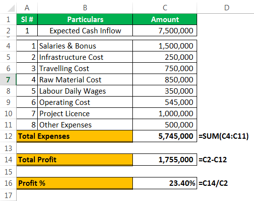
The expected cash flow from this project is $75 million, which is in cell C2. Total expenses comprise all your fixed and variable expenses, the total cost is $57.45 million in cell C12. Total profit is $17.55 million in cell C14, and profit % is 23.40% of your cash inflow.
It is the basic scenario of your project. Now, you need to know the profit scenario if some of your expenses increase or decrease.
Scenario 1
Scenario 2
- The “Project Cost” to be at $20 million
- The “Labor Daily Wages” to be at $5 million
- The “Operating Cost” is to be at $3.5 million
Now, you have listed out all the scenarios in the form. Based on these scenarios, you need to create a table about how it will impact your profit and profit %.
To create What-If Analysis scenarios, follow the below steps.
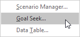
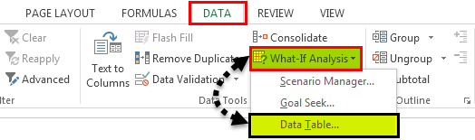
- Go to DATA > What-If Analysis > Scenario Manager.
Once you click “Scenario Manager,” it will show you below the dialog box.
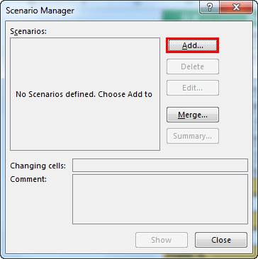
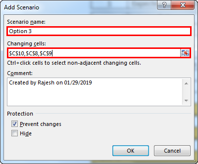
Click on “Add.” Then, give “Scenario name.”
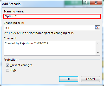
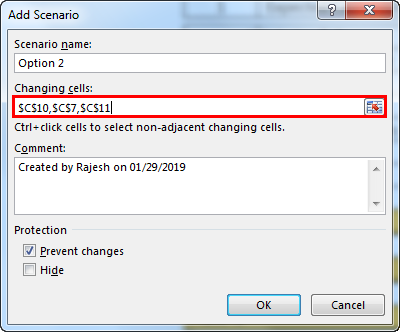
In changing cells, select the first scenario changes you have listed out. The changes are Project License (cell C10) at $15 million, Raw Material Cost (cell C7) at $11 million, and Other Expenses (cell C11) at $4.5 million. Mention these three cells here.
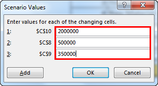
Click on “OK.” It will ask you to mention the new values as listed in scenario 1.
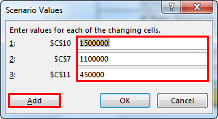
Do not click on “OK” but click on “OK Add.” It will save this scenario for you.
Now, it will ask you to create one more scenario. As we listed in scenario 2, make the changes. This time we need to change Project Cost (C10), Labour Cost (C8), and Operating Cost (C9).
Now, add new values here.
Now click on “OK.” It will show all the scenarios we have created.

Click on “Scenario summary.” It will ask you which result cells you want to change. Here, we need to change the Total Expense Cell (C12), Total Profit Cell (C14), and Profit % cell (C16).
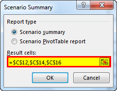
Click on “OK.” It will create a summary report for you in the new worksheet.
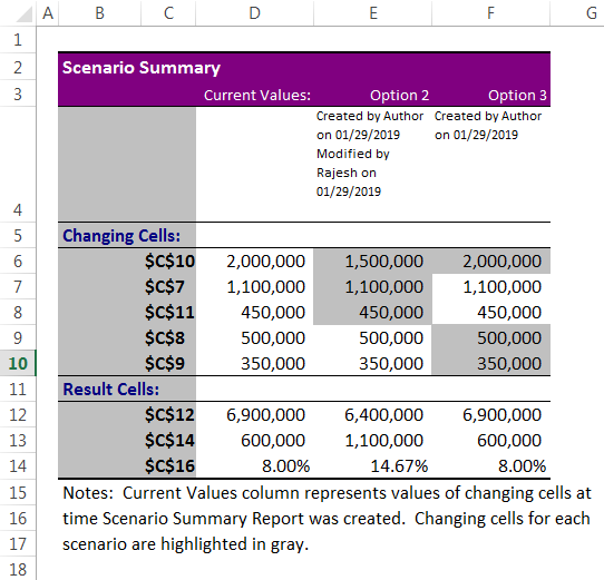
Total Excel has created three scenarios even though we have supplied only two scenario changes because Excel will show existing reports as one scenario.
From this table, we can easily see the impact of changes in pour profit %.
#2 Goal Seek in What-If Analysis
Now, we know the Scenario Manager’s advantage. What-if-Analysis Goal Seek can tell you what you must do to achieve the target.
Andrew is a class 10th student. His target is to achieve an average score of 85 in the final exam. He has already completed 5 exams and left with only 1 exam. Therefore, in the completed 5 exams.
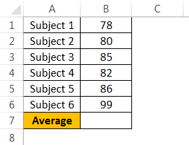
To calculate the current average, apply the average formula in the B7 cell.
The current average is 82.2.
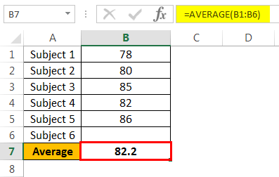
Andrew’s GOAL is 85. His current average is 82.2. He is short by 3.8 with one exam.
Now, the question is how much he has to score in the final exam to eventually get an overall average of 85. It can be found by the What-If Analysis GOAL SEEK tool.
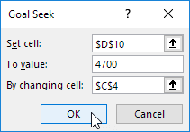
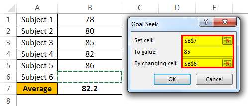
- Step 1: Go to DATA > What-If Analysis > Goal Seek.

- Step 2: It will show you below the dialog box.
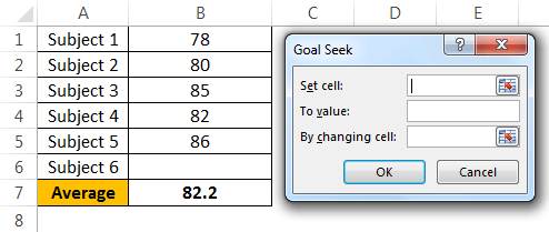
- Step 3: Here, we need to set the cell first. “Set cell” is nothing but which cell we need for the final result, i.e., our overall average cell (B7). Next is “To value.” Again, Andrew’s overall average GOAL is nothing but for what value we need to set the cell (85).
The next and final step is changing which cell you want to see the impact on. So, we need to change cell B6, the cell for the final subject’s score.
- Step 4: Click on “OK.” Excel will take a few seconds to complete the process, but it eventually shows the result like the one below.
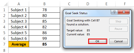
Now, we have our results here. To get an overall average of 85, Andrew has to score 99 in the final exam.
#3 Data Table in What-If Analysis
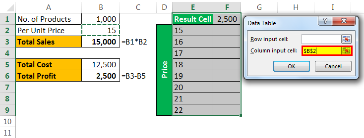
Assume you are selling 1,000 products at ₹15, your total anticipated expense is ₹12,500, and your profit is ₹2,500.
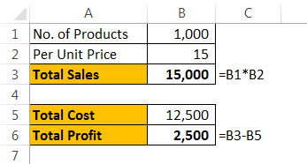
You are not happy with the profit you are getting. Your anticipated profit is ₹7,500. You have decided to increase your per-unit price to increase your profit, but you do not know how much you need to increase.
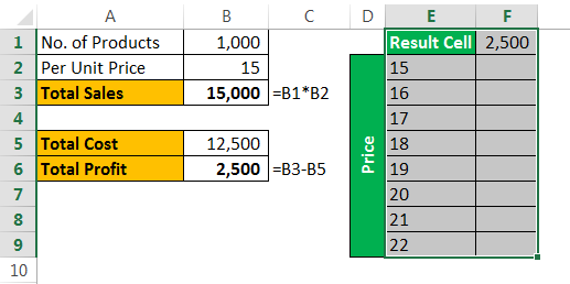
Data tables can help you. Create a table below.

Now, in the cell, F1 links to the “Total Profit” cell, B6.

- Step 1: Select the newly created table.
- Step 2: Go to DATA > What-if Analysis > Data Table.
- Step 3: Now, you will see below dialog box.
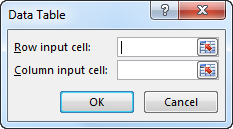
- Step 4: Since we are showing the result vertically, leave the ”Row input cell.” In the “Column input cell,” select cell B2, which is the original selling price.
- Step 5: Click on “OK” to get the results. It will list out profit numbers in the new table.
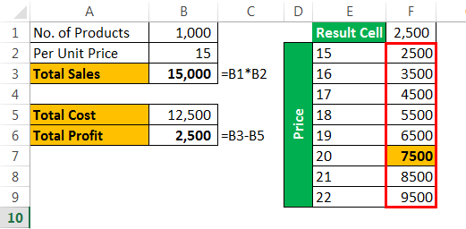
So, we have our Data Table ready. To profit from ₹7,500, you need to sell at ₹20 per unit.
Things to Remember
- The What-If Analysis data table can be performed with two variable changes. Refer to our article on What-If Analysis two-variable Data Table.
- What-If Analysis Goal Seek takes a few seconds to perform calculations.
- What-If Analysis Scenario Manager can give a summary with input numbers and current values together.
Recommended Articles
This article is a guide to What-If Analysis in Excel. Here, we discuss three types of What-If Analysis in Excel such as 1) Scenario Manager, 2) Goal Seek, 3) Data Tables along with practical examples, and a downloadable Excel template. You may learn more about Excel from the following articles: –
Источник