

Try it!
Use filters to temporarily hide some of the data in a table, so you can focus on the data you want to see.
Filter a range of data
-
Select any cell within the range.
-
Select Data > Filter.

-
Select the column header arrow
. -
Select Text Filters or Number Filters, and then select a comparison, like Between.
-
Enter the filter criteria and select OK.

 .
.

Filter data in a table
When you Create and format tables, filter controls are automatically added to the table headers.

-
Select the column header arrow
for the column you want to filter. -
Uncheck (Select All) and select the boxes you want to show.
-
Click OK.

The column header arrow  changes to a
  Filter icon. Select this icon to change or clear the filter.
Want more?
Filter data in a range or table
Filter data in a PivotTable
Need more help?
Want more options?
Explore subscription benefits, browse training courses, learn how to secure your device, and more.
Communities help you ask and answer questions, give feedback, and hear from experts with rich knowledge.
Advanced filter in Excel provides more opportunities for managing on data management spreadsheets. It is more complex in settings, but much more effective in action.
Using a standard filter, a Microsoft Excel user can solve not all of the tasks that are set. There is no visual display of the applied filtering conditions. It is not possible to apply more than two selection criteria. You can not filter the duplicate values to leave only unique records. And the criteria themselves are schematic and simple. The functionality of the extended filter is much richer. Let’s take a closer look at its possibilities.
How to make the advanced filter in Excel?
The advanced filter allows you to analysis data on an unlimited set of conditions. With this tool, the user can:
- to specify more than two selection criteria;
- to copy the result of filtering to another sheet;
- to set the condition of any complexity with the helping of formulas;
- to extract the unique values.
The algorithm for applying the extended filter is simple.
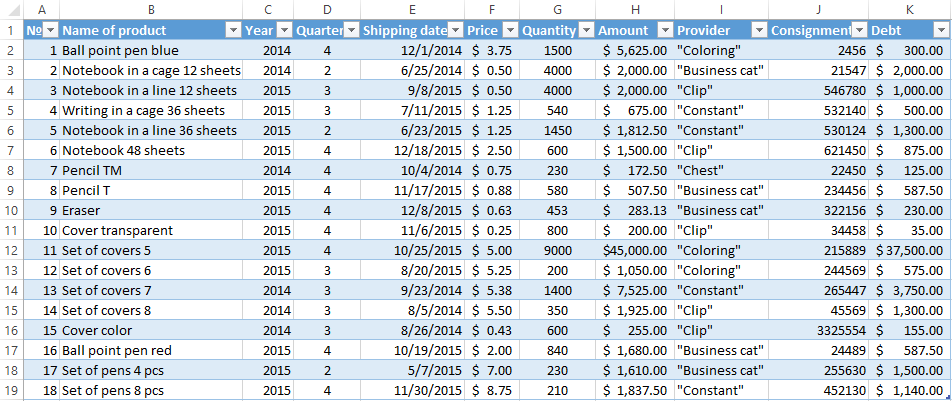
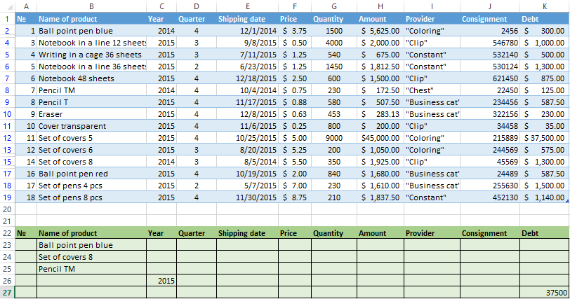
- To make the table with the original data or to open an existing one. Like so:
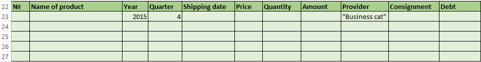
- To create the condition table. The features: the header line is the same with the «cap» of the filtered table. To avoid errors, need to copy the header line in the source table and paste it on the same sheet (side, top, underarm) or on another sheet. We enter the selection criteria into the condition table.
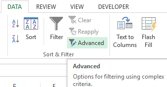
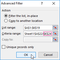
- Go to the «DATA» tab — «Sort and filter» — «Advanced». If the filtered information should be displayed on another sheet (NOT where the source table is), then you need to run the extended filter from another sheet.
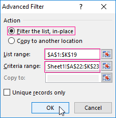
- In the «Advanced Filter» window that opens, to select the method of processing information (on the same sheet or on the other one), set the initial range (the table 1, example) and the range of conditions (the table 2, conditions). The header lines must be included in the ranges.
- To close the «Advanced Filter» window, click OK. We see the result.

The top table is the result of the filtering. The lower nameplate with the conditions is given for clarity near.
How to use the advanced filter in Excel?
To cancel the action of the advanced filter, we place the cursor anywhere in the table and press Ctrl + Shift + L or «DATA» — «Sort and Filter» — «Clear».
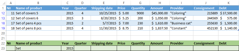
We will find using the «Advanced Filter» tool information on the values that contain the word «Set».
In the table of conditions we bring in the criteria. For example, these are:

The program in this case will search for all information on the goods, in the title of which there is the word «Set».
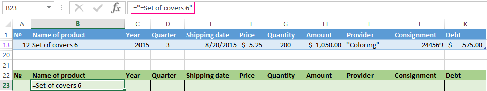
To search for the exact value, you can use the «=» sign. We enter the following criteria in the condition table:

Excel sees the «=» as a signal: the user will set the formula now. In order for the program to work correctly, the following should be written in the formula line: =»=Set of covers 6″.
After using the «Advanced Filter»:
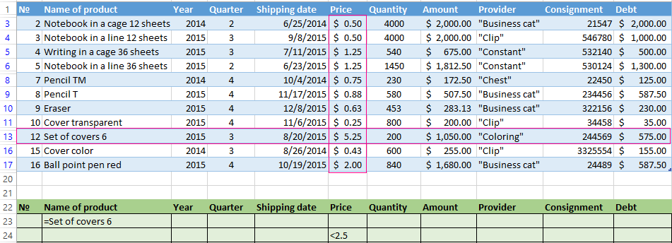
We filter the source table by the condition «OR» for different columns now. The operator «OR» is also in the tool «AutoFilter». But there it can be used within the single column.
In the condition label we introduce the selection criteria: =»=Set of covers 6″. (In the column «Name of product») and = «<2.5$» (in the column «Price»). That is, the program must select those values that contain the EXACTLY information about the good «Set of covers 6 ». OR to the information about the goods, which price is <2.5.

Please note: the criteria must be written under the corresponding headings in the DIFFERENT lines.
The result of selection:
The advanced filter allows you to use as a criterion of a formula. Let’s consider the example.

Selection of the line with the maximum indebtedness: =MAX(Table1[Debt]).
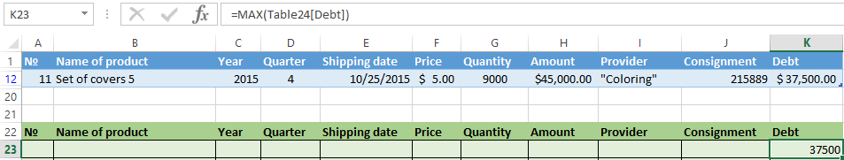
So we get the results as after running several filters on the one Excel sheet.
How to make few filters in Excel?
Let’s create the filter by several values. To do this, we enter in the table of conditions several criteria for selecting data:
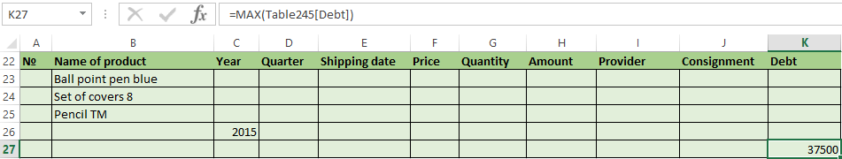
Apply the tool «Advanced Filter»:
Now from the table with the selected data we will extract new information, which was selected according to other criteria. There are only shipping date for autumn 2015 (from September to November). Example:
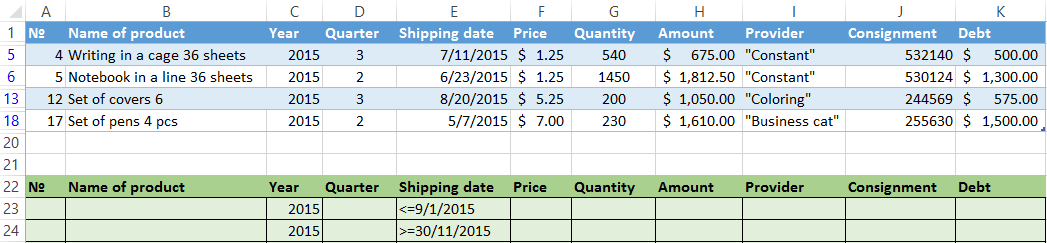
We introduce a new criterion in the condition table and apply the filtering tool. The initial range — is the table with data selected according to the previous criterion. This is how the filter is performed across on several columns.
To use few filters, you can create several condition tables on the new sheets. The method of implementation depends from the task which was set by user.
How to make the filter in Excel by lines?
By standard methods — you may not do it by any ways. Microsoft Excel selects data only in columns. Therefore, we need to look for other solutions.
Here are some examples of string criteria for the extended filter in Excel:
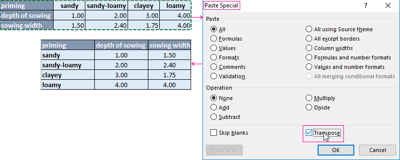
- Convert to the table. For example, from three rows make a list of three columns and apply the filtering to the transformed version.
- Use formulas to display exactly the data in the string that are needed. For example, make some indicator drop-down list. And in the next cell, enter the formula using the IF function. When a certain value is selected from the drop-down list, its parameter appears next to it.
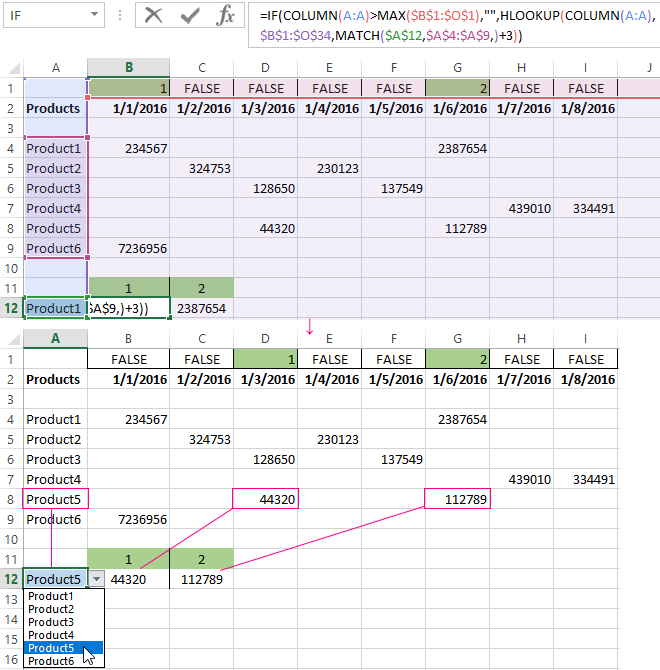
To give an example of how the filter works by rows in Excel, we are creating the label:
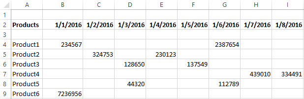
For the list of products, we create the drop-down list:
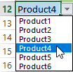
If necessary, learn how to create a drop-down list in Excel.
Above the table with the original data, we insert an empty line. In the cells, we introduce the formula that will show which columns the information is taken from.
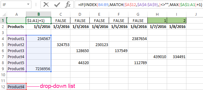
Next to the drop-down list box, we enter the following formula:
Its task is select from the table those values, that correspond to a certain good.
Download examples of advanced filtering
Thus, using the tool «Drop-down list» and built-in functions Excel selects data in rows according to a certain criterion.

Creating A Search Box In Excel
It’s unfortunate Excel does not have a form control search box (maybe in the future?) as I could see that type of tool opening the doors to a ton of creative and time-saving functionalities. But luckily there are a few different methods you can use to create a search box on your own.
In this post, I will walk you through a number of different ways you can create a professional-looking search box interface that can filter to only show desired search results within a data range.
Examples Of What We’ll Create:
Here is a little preview of the search interfaces you will be able to create after working through this article. All these solutions are included in the free Excel File download at the end of this article.
COMPATIBILITY NOTE: All non-VBA solutions will require the Filter Dynamic Array function. This function was released in Microsoft 365 and Excel 2021+.
Filtering Search Box — Single Column Search
In this section, you will learn how to create a filtering search box that provides results for an exact match result within a designated column of the data. You will also learn how to incorporate Option Buttons so that you have the flexibility to choose which column gets searched.
The end result will look something like this:

Spreadsheet Setup
In this example, the raw data is stored in a separate spreadsheet tab inside an Excel Table object (Ctrl + t). For clarity, I have renamed the table to DataTable.
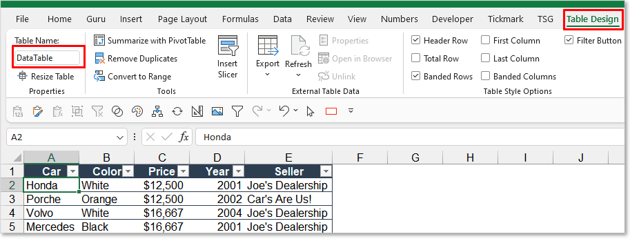
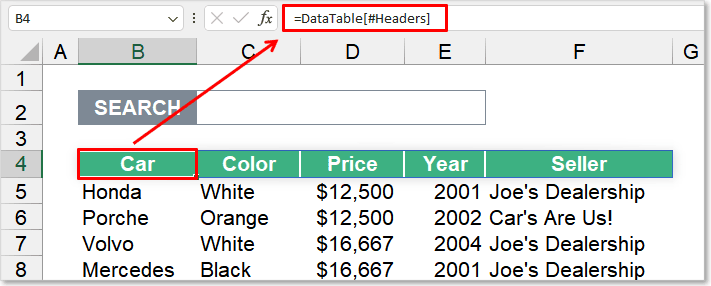
Table Header Formula
As part of this solution, you will need to either type out or bring over the header names from your source data table (in this example the Excel Table named DataTable). I chose to use a formula to dynamically bring over the heading names shown below.
Option Buttons To Choose Search Column
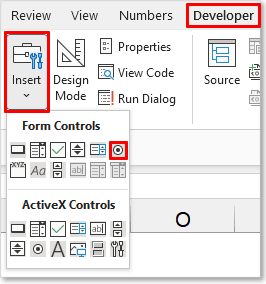
You can add Option Buttons to provide your user with an easy way to predetermine which column they would like to search through.
To add an Option Button to your spreadsheet, you will need to navigate to your Developer Tab in the Excel Ribbon. Once the Developer tab has been selected, you will need to open the Insert menu button and click the Option Button icon. You can then proceed to draw an Option Button control on your spreadsheet.
Once you’ve created an option button for each column you would like to search, you will likely want to change the label text to correspond with your data range’s column headings. You will need to ensure you align the order of your columns in the table with the order you created for the Option Buttons. For example, the header in Column 1 of your data range will be tied to the first Option Button you created on the spreadsheet.
If you would like to skip a column (for example, only search columns 1,2, & 4), create a total of 4 option buttons and hide the 3rd from sight, so your users cannot select it.
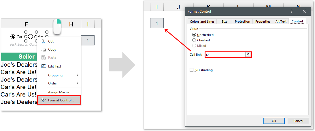
Lastly, you will need to link your Option Buttons to a cell on your spreadsheet. You can do this by
-
Right-clicking one of your Option Buttons
-
Select Format Control…
-
Populate the Cell Link textbox
-
Click OK
You will only need to do this one time as all Option Boxes on your spreadsheet will link to the same cell by default.
Table Body Formula For Filtered Data
Finally, you will need to write a formula for the search engine itself. This logic can be contained in a single Array Formula. There are 3 parts to this formula:
-
Filter Function — The Filter function allows you to perform a logic test within a column of a data range and return only the rows that pass the test. There is an optional third input for if there are no search results found where we will return the text “No Results Found”.
-
IsNumber/Search Functions — Since the Filter Function does not have a wildcard capability, there is a creative workaround we can use to give us this functionality. This allows us to perform partial-match or wildcard searches.
-
Index Function — This controls which column is getting searched. Because it points its column input to the output of your Option Buttons, it will allow the IsNumber/Search combination to only look at a single column within your data table.
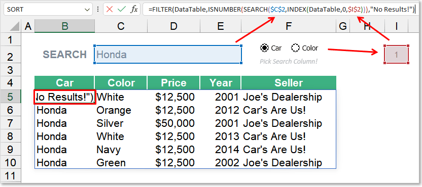
=FILTER(DataTable,ISNUMBER(SEARCH($C$2,INDEX(DataTable,0,$I$2))),»No Results!»)
Here is how the search engine formula has been integrated into our example. Notice that both the Search cell and the Option Button link cell are both referenced within the formula.
Filtering Search Box — Multiple Column Search Formula
In this section, you will learn how to create a filtering search box that loops through each column of your data range until it finds a match.
The end result will look something like this:
Spreadsheet Setup
In this example, the raw data is stored in a separate spreadsheet tab inside an Excel Table object (Ctrl + t). For clarity, I have renamed the table to DataTable.
Table Header Formula
As part of this solution, you will need to either type out or bring over the header names from your source data table (in this example the Excel Table named DataTable). I chose to use a formula to dynamically bring over the heading names shown below.
Table Body Formula For Filtered Data
Finally, you will need to write a formula for the search engine itself. This logic can be contained in a single Array Formula. There are 4 parts to this formula:
-
Filter Function — The Filter function allows you to perform a logic test within a column of a data range and return only the rows that pass the test. There is an optional third input for if there are no search results found where we will return the text “No Results Found”.
-
IsNumber/Search Functions — Since the Filter Function does not have a wildcard capability, there is a creative workaround we can use to give us this functionality. This allows us to perform partial-match or wildcard searches.
-
Index Function — This controls which column is getting searched. Because it points its column input to the output of your Option Buttons, it will allow the IsNumber/Search combination to only look at a single column within your data table.
-
Column Looping — To get a column looping or cycling effect for our search engine, we will actually need to perform our Filter Function multiple times (one for each column we wish to search through). Luckily, since the Filter function has an If_Empty input, we can simply execute another Filter function pointing to a new column if no results are found in the prior column.
Below is the formula used for our example. Notice the Filter function is repeated 5 times for the 5 columns in our data set. The formulas are the exact same except the Index function is referencing a different column number in each Filter function.
Ultimately, if there is nothing to filter after cycling through all five columns, a message stating “No Results!” is displayed to the user.
=FILTER(DataTable,ISNUMBER(SEARCH($C$2,INDEX(DataTable,0,1))),
FILTER(DataTable,ISNUMBER(SEARCH($C$2,INDEX(DataTable,0,2))),
FILTER(DataTable,ISNUMBER(SEARCH($C$2,INDEX(DataTable,0,3))),
FILTER(DataTable,ISNUMBER(SEARCH($C$2,INDEX(DataTable,0,4))),
FILTER(DataTable,ISNUMBER(SEARCH($C$2,INDEX(DataTable,0,5))),»No Results!»)))))
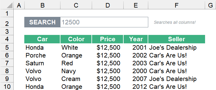
Here is how the search engine formula has been integrated into our example.

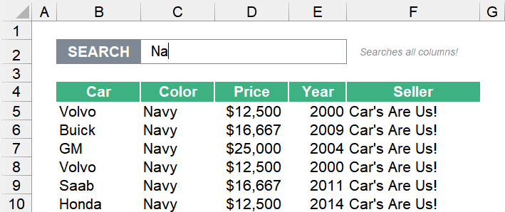
Filtering Search Box — As You Type
In this section, you will learn how to create a filtering search box that will provide filtered search results as you type in real-time. Similar to the prior solution, the search engine we build will loop through each column of your data until a match is found.
The end result will look something like this:
Spreadsheet Setup
In this example, the raw data is stored in a separate spreadsheet tab inside an Excel Table object (Ctrl + t). For clarity, I have renamed the table to DataTable.
Table Header Formula
As part of this solution, you will need to either type out or bring over the header names from your source data table (in this example the Excel Table named DataTable). I chose to use a formula to dynamically bring over the heading names shown below.
Add ActiveX TextBox
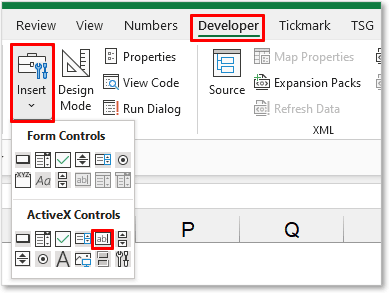
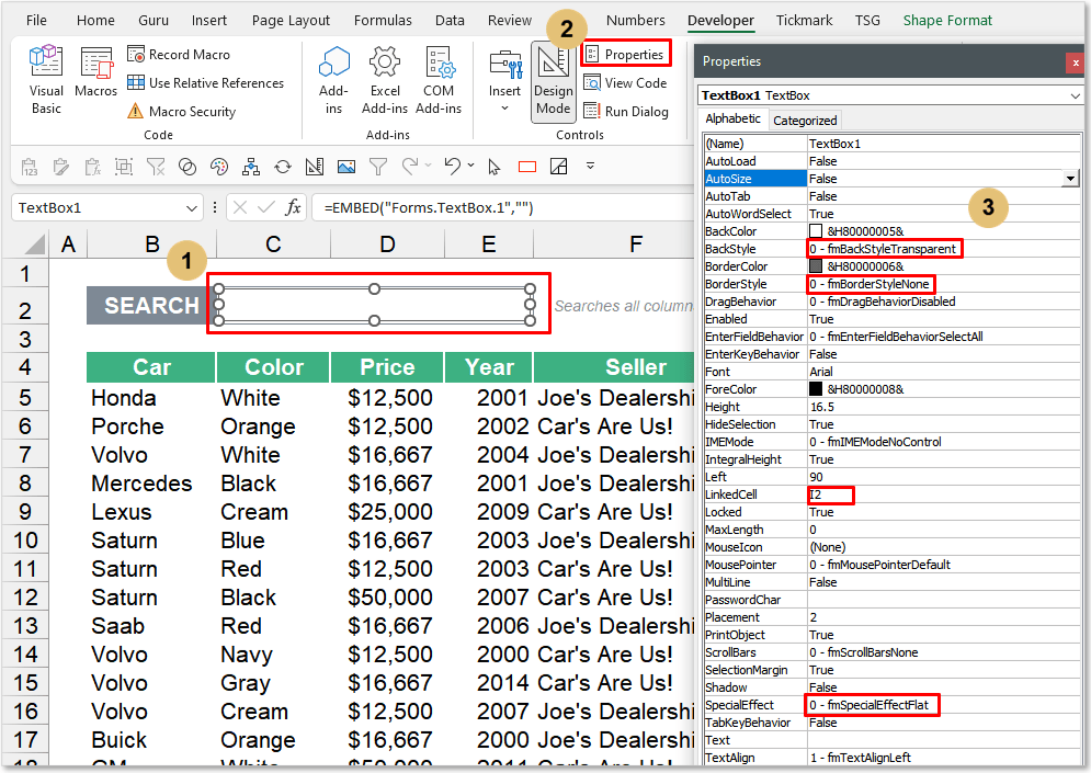
Table Body Formula For Filtered Data
We are going to utilize the same exact Excel formula for our filtering engine as we did in the prior solution (you can find more details about the logic here). The only difference will be that instead of pointing the Search function to the search box in Cell C2, we are going to point it to the cell we linked our ActiveX Textbox to (in this example, Cell I2).
Here is how the search engine formula has been integrated into our example.

=FILTER(DataTable,ISNUMBER(SEARCH($I$2,INDEX(DataTable,0,1))),
FILTER(DataTable,ISNUMBER(SEARCH($I$2,INDEX(DataTable,0,2))),
FILTER(DataTable,ISNUMBER(SEARCH($I$2,INDEX(DataTable,0,3))),
FILTER(DataTable,ISNUMBER(SEARCH($I$2,INDEX(DataTable,0,4))),
FILTER(DataTable,ISNUMBER(SEARCH($I$2,INDEX(DataTable,0,5))),»No Results!»)))))
Filtering Search Box — VBA Solution
Creating Your Search Box User Interface
Your search UI (user interface) can look however you want as long as there is a place for your user(s) to enter some text and a search button for them to click. The above image shows how I will typically create my UI. I use a nice clean textbox to hold the search text and a flat-styled, rounded rectangle shape for the button.
Get Fancy With Option Buttons
Instead of only allowing your users to filter on a single column, why not let them search through a few? By integrating Option Buttons with your search box you can have your users specify which column they want to search in. To insert the Option Buttons you will need to
-
Navigate to your Developer Tab in the Ribbon
-
Click the Insert dropdown button in the Controls group
-
Select the Option Button Form Control (first row, last icon)
-
Your mouse should now look like crosshairs and you will just want to click somewhere on your spreadsheet to draw the Option Button
After you draw a couple of Option Buttons, you can drag them into place so that they are relatively close to your search box. You can use the alignment tools to make everything look professional with even spacing.
One Pitfall
The one pitfall that I could not seem to get around is the fact that after entering your search text, you need to click outside of the textbox before you can click on the Search button. There are two workarounds that I could think of:
-
Instead of using a form control textbox, you can use either a Cell or ActiveX Textbox to hold the search text (I have lines of code in the below VBA macros commented out that can handle these situations)
-
Assign a keyboard shortcut to execute the macro, alleviating the need to click the Search button
I typically go the shortcut route as I like having the ability to place my search box wherever I want on my spreadsheet. Also, ActiveX controls can sometimes be glitchy depending on which version of Office you are using, so beware if you end up using this route.
Naming Your Objects
The key to getting this code to work well is to set up your objects (aka form controls) properly. First, you will need to determine the name of the text box that is holding your search term. To do this, you need to select the text box and then look at the Name Box (which is located to the left of the Formula Bar).
Typically you will see a default name of «Text Box 1», however, you can change this name to something more meaningful like «UserSearch». Make sure you hit the Enter key immediately after typing in your new name to apply the name change! If you click outside of the Name Box before hitting enter, your text box will revert back to its previous name.
For your Option Buttons, you will not need to change their object names (unless you really want to). You will, however, need to ensure that their text is verbatim with the data headings you will be filtering on. Notice how all my example Option Buttons have the exact same text as the headings in my data. This is EXTREMELY important as the VBA code below will be filtering based on the text associated with the selected Option Button.
Searching For Text Only
This macro will allow you to filter on any column with a text value within it. The macro uses an open-ended search (designated by the asterisk symbol before and after the search term). This means that you could search «whi» and the search would show any cell containing those 3 characters. If you want your search box to only filter on exactly what the user types, just remove the asterisks from the VBA code.
To set up this code with your data you will need to designate your data range for the variable DataRange and you will also need to modify your text box name inside the Shapes reference. If your data does not start in Column A you may need to add or subtract from the myField variable to ensure you are filtering on the correct column number associated with your data set.
Sub SearchBox()
‘PURPOSE: Filter Data on User-Determined Column & Text
‘SOURCE: www.TheSpreadsheetGuru.com
Dim myButton As OptionButton
Dim MyVal As Long
Dim ButtonName As String
Dim sht As Worksheet
Dim myField As Long
Dim DataRange As Range
Dim mySearch As Variant
‘Load Sheet into A Variable
Set sht = ActiveSheet
‘Unfilter Data (if necessary)
On Error Resume Next
sht.ShowAllData
On Error GoTo 0
‘Filtered Data Range (include column heading cells)
Set DataRange = sht.Range(«A4:E31») ‘Cell Range
‘Set DataRange = sht.ListObjects(«Table1»).Range ‘Table
‘Retrieve User’s Search Input
mySearch = sht.Shapes(«UserSearch»).TextFrame.Characters.Text ‘Control Form
‘mySearch = sht.OLEObjects(«UserSearch»).Object.Text ‘ActiveX Control
‘mySearch = sht.Range(«A1»).Value ‘Cell Input
‘Loop Through Option Buttons
For Each myButton In ActiveSheet.OptionButtons
If myButton.Value = 1 Then
ButtonName = myButton.Text
Exit For
End If
Next myButton
‘Determine Filter Field
On Error GoTo HeadingNotFound
myField = Application.WorksheetFunction.Match(ButtonName, DataRange.Rows(1), 0)
On Error GoTo 0
‘Filter Data
DataRange.AutoFilter _
Field:=myField, _
Criteria1:=»=*» & mySearch & «*», _
Operator:=xlAnd
‘Clear Search Field
sht.Shapes(«UserSearch»).TextFrame.Characters.Text = «» ‘Control Form
‘sht.OLEObjects(«UserSearch»).Object.Text = «» ‘ActiveX Control
‘sht.Range(«A1»).Value = «» ‘Cell Input
Exit Sub
‘ERROR HANDLERS
HeadingNotFound:
MsgBox «The column heading [» & ButtonName & «] was not found in cells » & DataRange.Rows(1).Address & «. » & _
vbNewLine & «Please check for possible typos.», vbCritical, «Header Name Not Found!»
End Sub
Searching For Text & Numerical Values
This VBA code is the exact same setup as the previous code but it has a few extra lines added to handle both numerical and text inputs from your user.
Sub SearchBox()
‘PURPOSE: Filter Data on User-Determined Column & Text/Numerical value
‘SOURCE: www.TheSpreadsheetGuru.com
Dim myButton As OptionButton
Dim SearchString As String
Dim ButtonName As String
Dim sht As Worksheet
Dim myField As Long
Dim DataRange As Range
Dim mySearch As Variant
‘Load Sheet into A Variable
Set sht = ActiveSheet
‘Unfilter Data (if necessary)
On Error Resume Next
sht.ShowAllData
On Error GoTo 0
‘Filtered Data Range (include column heading cells)
Set DataRange = sht.Range(«A4:E31») ‘Cell Range
‘Set DataRange = sht.ListObjects(«Table1»).Range ‘Table
‘Retrieve User’s Search Input
mySearch = sht.Shapes(«UserSearch»).TextFrame.Characters.Text ‘Control Form
‘mySearch = sht.OLEObjects(«UserSearch»).Object.Text ‘ActiveX Control
‘mySearch = sht.Range(«A1»).Value ‘Cell Input
‘Determine if user is searching for number or text
If IsNumeric(mySearch) = True Then
SearchString = «=» & mySearch
Else
SearchString = «=*» & mySearch & «*»
End If
‘Loop Through Option Buttons
For Each myButton In sht.OptionButtons
If myButton.Value = 1 Then
ButtonName = myButton.Text
Exit For
End If
Next myButton
‘Determine Filter Field
On Error GoTo HeadingNotFound
myField = Application.WorksheetFunction.Match(ButtonName, DataRange.Rows(1), 0)
On Error GoTo 0
‘Filter Data
DataRange.AutoFilter _
Field:=myField, _
Criteria1:=SearchString, _
Operator:=xlAnd
‘Clear Search Field
sht.Shapes(«UserSearch»).TextFrame.Characters.Text = «» ‘Control Form
‘sht.OLEObjects(«UserSearch»).Object.Text = «» ‘ActiveX Control
‘sht.Range(«A1»).Value = «» ‘Cell Input
Exit Sub
‘ERROR HANDLERS
HeadingNotFound:
MsgBox «The column heading [» & ButtonName & «] was not found in cells » & DataRange.Rows(1).Address & «. » & _
vbNewLine & «Please check for possible typos.», vbCritical, «Header Name Not Found!»
End Sub
Linking Your VBA Code To The Search Button
Once you have added your VBA code to your spreadsheet and are ready to see it in action, you will need to turn your search button into a trigger for your macro code. To do this, simply right-click on your button and select Assign Macro. The Assign Macro Dialog Box will pop up and you will want to find & select your macro’s name (in this case «Searchbox»). Once you have highlighted your macro name and clicked OK, every time you click your search button your filtering macro will run.
Creating A «Clear Filter» Button
You may want to add a feature to clear your filter on your search data. All you need to do is create another button and link the below code to your Clear Filter button
Sub ClearFilter()
‘PURPOSE: Clear all filter rules
‘Clear filters on ActiveSheet
On Error Resume Next
ActiveSheet.ShowAllData
On Error GoTo 0
End Sub
Get The Example File
If you would like to get a copy of the Excel file I used throughout this article, feel free to directly download the file by clicking the download button below.

About The Author
Hey there! I’m Chris and I run TheSpreadsheetGuru website in my spare time. By day, I’m actually a finance professional who relies on Microsoft Excel quite heavily in the corporate world. I love taking the things I learn in the “real world” and sharing them with everyone here on this site so that you too can become a spreadsheet guru at your company.
Through my years in the corporate world, I’ve been able to pick up on opportunities to make working with Excel better and have built a variety of Excel add-ins, from inserting tickmark symbols to automating copy/pasting from Excel to PowerPoint. If you’d like to keep up to date with the latest Excel news and directly get emailed the most meaningful Excel tips I’ve learned over the years, you can sign up for my free newsletters. I hope I was able to provide you with some value today and I hope to see you back here soon!
— Chris
Founder, TheSpreadsheetGuru.com