
-
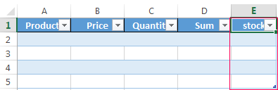
Create a table
Video
-
Sort data in a table
Video
-
Filter data in a range or table
Video
-
Add a Total row to a table
Video
-
Use slicers to filter data
Video
Sign in with Microsoft
Sign in or create an account.
Hello,
Select a different account.
You have multiple accounts
Choose the account you want to sign in with.
Thank you for your feedback!
×
Convert Data Into a Table in Excel
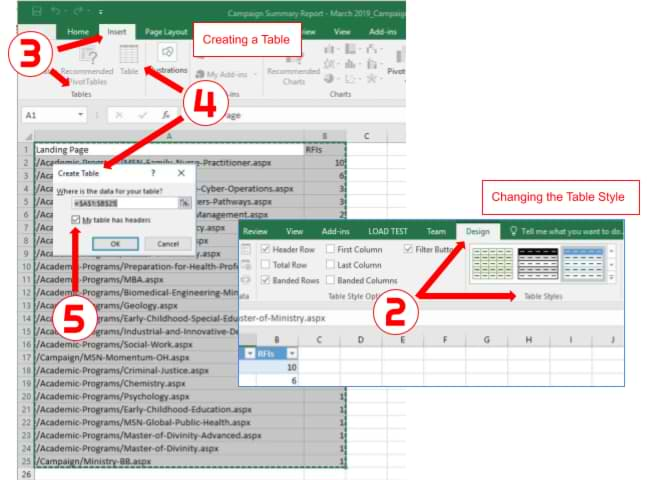
This page will show you how to convert Excel data into a table.
Creating a Table within Excel
- Open the Excel spreadsheet.
- Use your mouse to select the cells that contain the information for the table.
- Click the «Insert» tab > Locate the «Tables» group.
- Click «Table». A «Create Table» dialog box will open.
- If you have column headings, check the box «My table has headers».
- Verify that the range is correct > Click [OK].
- Resize your columns to make the headings visible.
Changing the Table Style
- Click on a cell in the table to activate the «Table Tools» tab.
- Click the «Design» tab > Locate the «Table Styles» group.
- Choose a style/color option that appeals to you. (Hover over the various table styles to see a live preview.)
Keywords: Office, color, colors, filter, sort, rows, columns, apply, enhance, table
Share This Post
-
Facebook
-
Twitter
-
LinkedIn
Blog Resources
Cedarville offers more than 150 academic programs to grad, undergrad, and online students. Cedarville is known for its biblical worldview, academic excellence, intentional discipleship, and authentic Christian community.

Loading…
Содержание
- Create and format tables
- Try it!
- Data Tables
- One Variable Data Table
- Two Variable Data Table
- How to make and use a data table in Excel
- What is a data table in Excel?
- How to create a one variable data table in Excel
- Row-oriented data table
- How to make a two variable data table in Excel
- Data table to compare multiple results
- Data table in Excel — 3 things you should know
- How to delete a data table in Excel
- How to edit data table results
- How to recalculate data table manually
Create and format tables
Create and format a table to visually group and analyze data.
Note: Excel tables shouldn’t be confused with the data tables that are part of a suite of What-If Analysis commands ( Forecast, on the Data tab). See Introduction to What-If Analysis for more information.

Try it!
Select a cell within your data.
Select Home > Format as Table.
Choose a style for your table.
In the Create Table dialog box, set your cell range.
Mark if your table has headers.
Insert a table in your spreadsheet. See Overview of Excel tables for more information.
Select a cell within your data.
Select Home > Format as Table.
Choose a style for your table.
In the Create Table dialog box, set your cell range.
Mark if your table has headers.
To add a blank table, select the cells you want included in the table and click Insert > Table.
To format existing data as a table by using the default table style, do this:
Select the cells containing the data.
Click Home > Table > Format as Table.
If you don’t check the My table has headers box, Excel for the web adds headers with default names like Column1 and Column2 above the data. To rename a default header, double-click it and type a new name.
Note: You can’t change the default table formatting in Excel for the web.
Источник
Data Tables
Instead of creating different scenarios, you can create a data table to quickly try out different values for formulas. You can create a one variable data table or a two variable data table.
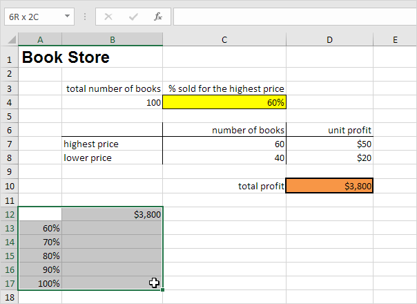
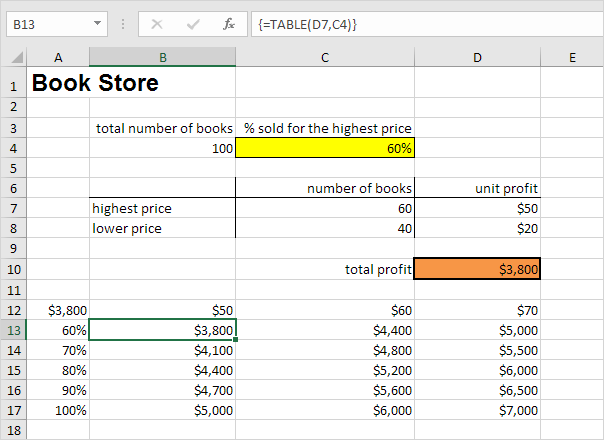
Assume you own a book store and have 100 books in storage. You sell a certain % for the highest price of $50 and a certain % for the lower price of $20. If you sell 60% for the highest price, cell D10 below calculates a total profit of 60 * $50 + 40 * $20 = $3800.
One Variable Data Table
To create a one variable data table, execute the following steps.
1. Select cell B12 and type =D10 (refer to the total profit cell).
2. Type the different percentages in column A.
3. Select the range A12:B17.
We are going to calculate the total profit if you sell 60% for the highest price, 70% for the highest price, etc.
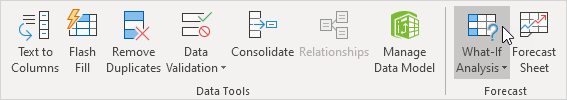
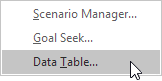
4. On the Data tab, in the Forecast group, click What-If Analysis.
5. Click Data Table.
6. Click in the ‘Column input cell’ box (the percentages are in a column) and select cell C4.
We select cell C4 because the percentages refer to cell C4 (% sold for the highest price). Together with the formula in cell B12, Excel now knows that it should replace cell C4 with 60% to calculate the total profit, replace cell C4 with 70% to calculate the total profit, etc.
Note: this is a one variable data table so we leave the Row input cell blank.
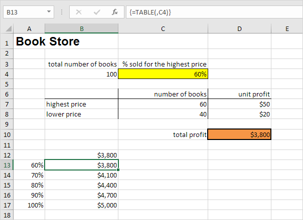
Conclusion: if you sell 60% for the highest price, you obtain a total profit of $3800, if you sell 70% for the highest price, you obtain a total profit of $4100, etc.
Note: the formula bar indicates that the cells contain an array formula. Therefore, you cannot delete a single result. To delete the results, select the range B13:B17 and press Delete.
Two Variable Data Table
To create a two variable data table, execute the following steps.
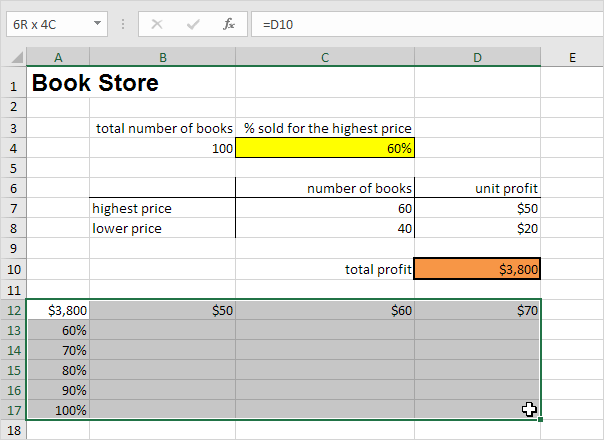
1. Select cell A12 and type =D10 (refer to the total profit cell).
2. Type the different unit profits (highest price) in row 12.
3. Type the different percentages in column A.
4. Select the range A12:D17.
We are going to calculate the total profit for the different combinations of ‘unit profit (highest price)’ and ‘% sold for the highest price’.
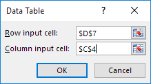
5. On the Data tab, in the Forecast group, click What-If Analysis.
6. Click Data Table.
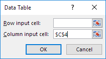
7. Click in the ‘Row input cell’ box (the unit profits are in a row) and select cell D7.
8. Click in the ‘Column input cell’ box (the percentages are in a column) and select cell C4.
We select cell D7 because the unit profits refer to cell D7. We select cell C4 because the percentages refer to cell C4. Together with the formula in cell A12, Excel now knows that it should replace cell D7 with $50 and cell C4 with 60% to calculate the total profit, replace cell D7 with $50 and cell C4 with 70% to calculate the total profit, etc.
Conclusion: if you sell 60% for the highest price, at a unit profit of $50, you obtain a total profit of $3800, if you sell 80% for the highest price, at a unit profit of $60, you obtain a total profit of $5200, etc.
Note: the formula bar indicates that the cells contain an array formula. Therefore, you cannot delete a single result. To delete the results, select the range B13:D17 and press Delete.
Источник
How to make and use a data table in Excel
 by Svetlana Cheusheva, updated on March 16, 2023
The tutorial shows how to use data tables for What-If analysis in Excel. Learn how to create a one-variable and two-variable table to see the effects of one or two input values on your formula, and how to set up a data table to evaluate multiple formulas at once.
You have built a complex formula dependent on multiple variables and want to know how changing those inputs changes the results. Instead of testing each variable individually, make a What-if analysis data table and observe all possible outcomes with a quick glance!
What is a data table in Excel?
In Microsoft Excel, a data table is one of the What-If Analysis tools that allows you to try out different input values for formulas and see how changes in those values affect the formulas output.
Data tables are especially useful when a formula depends on several values, and you’d like to experiment with different combinations of inputs and compare the results.
Currently, there exist one variable data table and two variable data table. Although limited to a maximum of two different input cells, a data table enables you to test as many variable values as you want.
Note. A data table isn’t the same thing as an Excel table, which is purposed for managing a group of related data. If you are looking to learn about many possible ways to create, clear and format a regular Excel table, not data table, please check out this tutorial: How to make and use a table in Excel.
How to create a one variable data table in Excel
One variable data table in Excel allows testing a series of values for a single input cell and shows how those values influence the result of a related formula.
To help you better understand this feature, we are going to follow a specific example rather than describing generic steps.
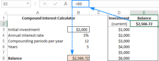
Suppose you are considering depositing your savings in a bank, which pays 5% interest that compounds monthly. To check different options, you’ve built the following compound interest calculator where:
- B8 contains the FV formula that calculates the closing balance.
- B2 is the variable you want to test (initial investment).

And now, let’s do a simple What-If analysis to see what your savings will be in 5 years depending on the amount of your initial investment, ranging from $1,000 to $6,000.
Here are the steps to make a one-variable data table:
- Enter the variable values either in one column or across one row. In this example, we are going to create a column-oriented data table, so we type our variable values in a column (D3:D8) and leave at least one blank column to the right for the outcomes.
- Type your formula in the cell one row above and one cell to the right of the variable values (E2 in our case). Or, link this cell to the formula in your original dataset (if you decide to change the formula in the future, you would need to update only one cell). We choose the latter option, and enter this simple formula in E2: =B8

Tip. If you want to examine the impact of the variable values on other formulas that refer to the same input cell, enter the additional formula(s) to the right of the first formula, as shown in this example.
Now, you can take a quick look at your one-variable data table, examine the possible balances and choose the optimal deposit size: 
Row-oriented data table
The above example shows how to set up a vertical, or column-oriented, data table in Excel. If you prefer a horizontal layout, here’s what you need to do:
- Type the variable values in a row, leaving at least one empty column to the left (for the formula) and one empty row below (for the results). For this example, we enter the variable values in cells F3:J3.
- Enter the formula in the cell that is one column to the left of your first variable value and one cell below (E4 in our case).
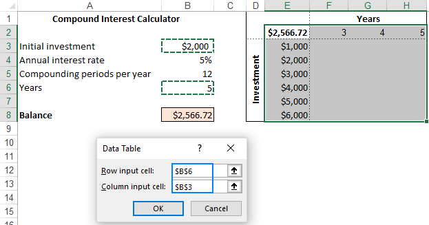
- Make a data table as discussed above, but enter the input value (B3) in the Row input cell box:
- Click OK, and you will have the following result:


How to make a two variable data table in Excel
A two-variable data table shows how various combinations of 2 sets of variable values affect the formula result. In other words, it shows how changing two input values of the same formula changes the output.
The steps to create a two-variable data table in Excel are basically the same as in the above example, except that you enter two ranges of possible input values, one in a row and another in a column.
To see how it works, let’s use the same compound interest calculator and examine the effects of the size of the initial investment and the number of years on the balance. To have it done, set up your data table in this way:
- Enter your formula in a blank cell or link that cell to your original formula. Make sure you have enough empty columns to the right and empty rows below to accommodate your variable values. As before, we link the cell E2 to the original FV formula that calculates the balance: =B8
- Type one set of input values below the formula, in the same column (investment values in E3:E8).
- Enter the other set of variable values to the right of the formula, in the same row (number of years in F2:H2).
At this point, your two variable data table should look similar to this: 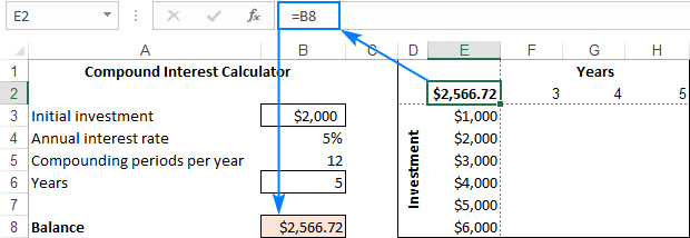

Data table to compare multiple results
If you wish to evaluate more than one formula at the same time, build your data table as shown in the previous examples, and enter the additional formula(s):
- To the right of the first formula in case of a vertical data table organized in columns
- Below the first formula in case of a horizontal data table organized in rows
For the «multi-formula» data table to work correctly, all the formulas should refer to the same input cell.
As an example, let’s add one more formula to our one-variable data table to calculate the interest and see how it is affected by the size of the initial investment. Here’s what we do:
- In cell B10, compute the interest with this formula: =B8-B3
- Arrange the data table’s source data like we did earlier: variable values in D3:D8 and E2 linked to B8 (Balance formula).
- Add one more column to the data table range (column F), and link F2 to B10 (interest formula):
- Select the extended data table range (D2:F8).
- Open the Data Table dialog box by clicking Data tab >What-If Analysis>Data Table…
- In the Column Input cell box, supply the input cell (B3), and click OK.

VoilГ , you can now observe the effects of your variable values on both formulas: 
Data table in Excel — 3 things you should know
To effectively use data tables in Excel, please keep in mind these 3 simple facts:
- For a data table to be created successfully, the input cell(s) must be on the same sheet as the data table.
- Microsoft Excel uses the TABLE(row_input_cell, colum_input_cell) function to calculate data table results:
- In one-variable data table, one of the arguments is omitted, depending on the layout (column-oriented or row-oriented). For example, in our horizontal one-variable data table, the formula is =TABLE(, B3) where B3 is the column input cell.
- In two-variable data table, both arguments are in place. For example, =TABLE(B6, B3) where B6 is the row input cell and B3 is the column input cell.
The TABLE function is entered as an array formula. To make sure of this, select any cell with the calculated value, look at the formula bar, and note the around the formula. However, it is not a normal array formula — you can’t type it in the formula bar nor can you edit an existing one. It is just «for show».
How to delete a data table in Excel
As mentioned above, Excel does not allow deleting values in individual cells containing the results. Whenever you try to do this, an error message «Cannot change part of a data table» will show up.
However, you can easily clear the entire array of the resulting values. Here’s how:
- Depending on your needs, select all the data table cells or only the cells with the results.
- Press the Delete key.
How to edit data table results
Since it is not possible to change part of an array in Excel, you cannot edit individual cells with calculated values. You can only replace all those values with your own one by performing these steps:
- Select all the resulting cells.
- Delete the TABLE formula in the formula bar.
- Type the desired value, and press Ctrl + Enter .
This will insert the same value in all the selected cells: 
Once the TABLE formula is gone, the former data table becomes a usual range, and you are free to edit any individual cell normally.
How to recalculate data table manually
If a large data table with multiple variable values and formulas slows down your Excel, you can disable automatic recalculations in that and all other data tables.
For this, go to the Formulas tab > Calculation group, click the Calculation Options button, and then click Automatic Except Data Tables. 
This will turn off automatic data table calculations and speed up recalculations of the entire workbook.
To manually recalculate your data table, select its resulting cells, i.e. the cells with TABLE() formulas, and press F9 .
This is how you create and use a data table in Excel. To have a closer look at the examples discussed this this tutorial, you are welcome to download our sample Excel Data Tables workbook. I thank you for reading and would be happy to see you again next week!
Источник
Microsoft Excel is convenient for creating tables and doing calculations. Its working area is a set of cells to be filled with data. Consequently, the data can be formatted, used for building graphs, charts, summary reports.
For a beginner, working with tables in Excel may seem complicated at the first glance. It is differs considerably from the principles of table construction in Word. However, let us start from the very basics: creating and formatting tables. By the time you reach the end of this article, you will understand there is no better tool for creating tables than Excel.
Creating a table in Excel: a dummy’s guide
Working with Excel tables for dummies does not tolerate haste. There are different ways to create a table for a specific purpose, and each of them has its advantages. Therefore, let us start with assessing the situation visually.
Look carefully at the work sheet of the table processor:
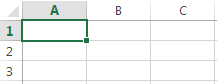
It is a set of cells in columns and rows. Essentially, it’s a table. The columns are marked with letters. The rows are designated with numbers. There are no borders.
First of all, let’s learn to work with cells, rows and columns.
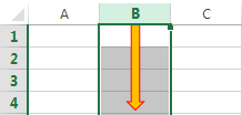
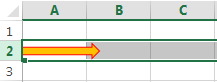
How to select a column and a row
To select the entire column, left-click on the letter that marks it.
To select a row, click on the number it’s designated with.
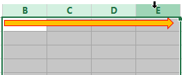
To select several columns or rows, left-click on the name, hold down the button and drag the pointer.
To select a column with the help of hot keys, place the cursor in any cell of the column and press Ctrl + Space. The key combination Shift + Space is used to select a row.
How to resize cells
If your information does not fit in the table, you need to resize the cells.
- You can move them manually by grabbing the cell boundary with the left mouse button.
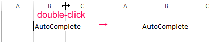
- If the cell contains a long word, you can double-click on the boundary of the column/row. The program will expand its boundary automatically.
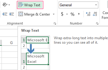
- If you need to increase the height of a row preserving the column width, use the button «Wrap Text» in the tool bar.
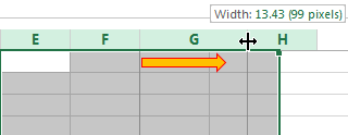
To change the column width and the row height in a certain range, resize 1 column/row (by dragging its boundaries manually) – and all the selected columns and rows will be resized automatically.
Important note. To go back to the previous size, you can press the «Undo Typing» button or the hot-key combination CTRL+Z. However, it works only if used immediately. Later on, it will not help.
To bring the rows to their initial boundaries, open the tool menu: «HOME»-«Format» and choose «AutoFit Row Height».
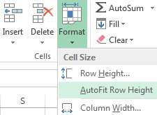
This method does not work for columns. Click «Format» — « AutoFit Row Width» Memorize this number. Select any cell in the column that needs to go back to the initial size. Click «Format» — «Column Width» again and enter the value suggested by the program (as a rule, it’s 8.43 – the number of characters in the Calibri font, size 11 pt). OK.
How to insert a column or row
Select the column/row to the right of/below the place where the insertion needs to be made. That is, the new column will appear to the left of the selected cell. The new row will be pasted above it.
Right-click on the cell and select «Insert» in the drop-down menu (or hit the hot-key combination CTRL+SHIFT+»=»).
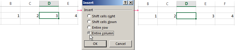
Select «Entire column» and press OK.
Hint. To insert a new column quickly, select a column in the desired position and hit CTRL+SHIFT+PLUS.
All these skills will come handy when building a table in Excel. You will need to resize the cells and insert rows/columns in the process.
Creating a table with formulas step by step
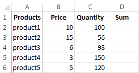
- Fill in the header manually by entering the column headings. Fill in the rows by entering your data. Apply the acquired knowledge in practice: expand the column boundaries, adjust the row height.
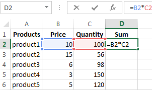
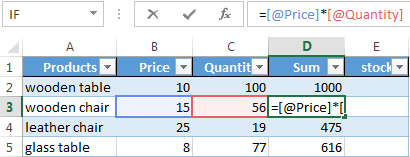
- To fill in the «Sum» column, place the cursor in its first cell. Enter «=». In such a way, we inform Excel: a formula will be here. Select the cell B2 (with the first price). Enter the multiplication symbol (*). Select the cell C2 (with the quantity). Press ENTER.
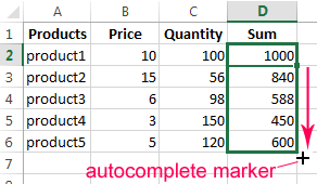
- When you hover the pointer over the cell containing the formula, a small cross will appear in its bottom right corner. It points out the autocomplete marker. Grab it with the left mouse button and drag it to the end of the column. The formula will be copied into every cell.
- Designate the boundaries of your table. Select the range containing your data. Click the button «HOME»-«Border» (on the main page in the «Font» menu). And click «All Borders».
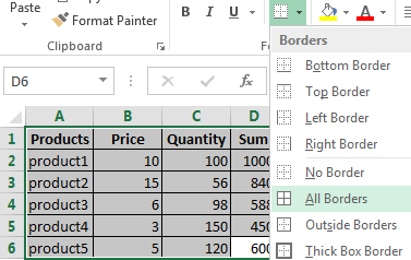
Now the column and row borders will be visible when you print the table.
The «Font» menu allows you to format the data in your Excel table the way you would do it in Word.
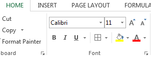
For example, change the font size and highlight the header in bold. You may also apply center alignment, word wrap, etc.
Creating a table in Excel: a step-by-step instruction
You already know the simplest way to create tables. However, Excel can offer a more convenient variant (in terms of the subsequent formatting and work with the data).
Let us construct a smart (dynamic) table:
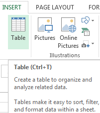
- Go to the «INSERT» tab – the «Table» tool (or press the hot-key combination CTRL+T).
- This will open a dialog window, in which you need to enter the data range. Check the box for a table with headings. Click OK. It’s no big deal if you don’t enter the proper range on the first try. The smart table is flexible, dynamic.
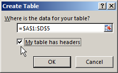
Important note. You can also take an alternative route: start with selecting the range of cells, then press the «Table» button.
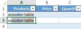
Now enter your data into the ready framework. If you need an additional column, place the cursor in the heading cell. Make the entry and press ENTER. The range will expand automatically.

If you need additional rows, grab the autocomplete marker in the bottom right corner and drag it downward.
How to work with a table in Excel
With the release of new versions of the program, working with tables in Excel has become more interesting and dynamic. After a smart table has been formed on the spreadsheet, the tool «TABLE TOOLS» — «DESIGN» becomes available.
Here you can name the table or resize it.
Various styles are available to you, as well as the opportunity to transform the table into a regular range or a consolidated sheet.
MS Excel dynamic electronic tables offer immense opportunities. Let us begin with the basic skills of data entry and autocompletion:
- Select a cell by clicking on it with the left mouse button. Enter the text/numeric value. Press ENTER. If you need to change the value, place the cursor in the cell again and enter the new data.
- When you enter a value repetitively, Excel will recognize it. You will only need to enter several symbols and press enter.
- In a smart table, to apply a formula to the entire column, enter it in the first cell. The program will copy the formula in other cells automatically.
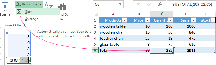
- To calculate the totals, select the column containing the values plus an empty cell for the future total and click the «Sum» button (the «Editing» tool group on the «HOME» tab, or press the hot-key combination ALT+»=»).
When you click on the little arrow to the right of every subheading in the header, you obtain access to the additional tools for working with the data in the table.
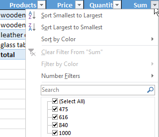
Sometimes the user has to work with huge tables, in which you need to scroll several thousand rows to see the totals. Deleting the rows is not an option (you will still need the data later). However, you can hide them. To this end, use number filters (depicted in the image above). Uncheck the values that need to be hidden.