
Содержание
- How to Create a Report in Excel
- In This Article
- What to Know
- Creating Basic Charts and Tables for an Excel Report
- Using PivotTables to Generate a Report From an Excel Spreadsheet
- How to Print Your Excel Report
- How to Create a Report in Excel: The PivotTable
- PRYOR+ 7-DAYS OF FREE TRAINING
- Create status and trend reports from a work item query
- Prerequisites
- Create an Excel report from a flat-list query
- Create a query-based report by using Excel
- Q: Can I export a query to Excel?
- Q: Which fields can’t I use to generate a report?
- Q: Can I create reports if I’m working in Azure DevOps?
- Q: How do I refresh the report to show the most recent data?
How to Create a Report in Excel
Using charts, graphs, and pivot tables makes it easy
:max_bytes(150000):strip_icc()/RyanDube-214359-8f50cb3133cd47c7ae1f3d4f09349f4e.JPG)
In This Article
Jump to a Section
What to Know
- Create a report using charts: Select Insert >Recommended Charts, then choose the one you want to add to the report sheet.
- Create a report with pivot tables: Select Insert >PivotTable. Select the data range you want to analyze in the Table/Range field.
- Print: Go to File >Print, change the orientation to Landscape, scaling to Fit All Columns on One Page, and select Print Entire Workbook.
This article explains how to create a report in Microsoft Excel using key skills like creating basic charts and tables, creating pivot tables, and printing the report. The information in this article applies to Excel 2019, Excel 2016, Excel 2013, Excel 2010, and Excel for Mac.
Creating Basic Charts and Tables for an Excel Report
Creating reports usually means collecting information and presenting it all in a single sheet that serves as the report sheet for all of the information. These report sheets should be formatted in a way that’s easy to print as well.
One of the most common tools people use in Excel to create reports is the chart and table tools. To create a chart in an Excel report sheet:
Select Insert from the menu, and in the charts group, select the type of chart you want to add to the report sheet.
:max_bytes(150000):strip_icc()/001-how-to-create-a-report-in-excel-3384b6a8655f46d194f9a6c4e66f8267.jpg)
In the Chart Design menu, in the Data group, select Select Data.
:max_bytes(150000):strip_icc()/002-how-to-create-a-report-in-excel-ae2e9c1538e84d9e979d564addf9ef8b.jpg)
Select the sheet with the data and select all cells containing the data you want to chart (include headers).
:max_bytes(150000):strip_icc()/003-how-to-create-a-report-in-excel-fb008687c1694cca980abec23c313112.jpg)
The chart will update in your report sheet with the data. The headers will be used to populate the labels in the two axis.
:max_bytes(150000):strip_icc()/how-to-create-a-report-in-excel-4691111-4-23f0e5d9ab484e1caa2bd8f05c1e85e6.png)
Repeat the above steps to create new charts and graphs that appropriately represent the data you want to show in your report. When you need to create a new report, you can just paste the new data into the data sheets, and the charts and graphs update automatically.
:max_bytes(150000):strip_icc()/how-to-create-a-report-in-excel-4691111-5-db599f2149f54e4c87a2d2a0509c6b71.png)
There are different ways to lay out a report using Excel. You can include graphs and charts on the same page as tabular (numeric) data, or you can create multiple sheets so visual reporting is on one sheet, tabular data is on another sheet, and so on.
Using PivotTables to Generate a Report From an Excel Spreadsheet
Pivot tables are another powerful tool for creating reports in Excel. Pivot tables help with digging more deeply into data.
Select the sheet with the data you want to analyze. Select Insert > PivotTable.
:max_bytes(150000):strip_icc()/006-how-to-create-a-report-in-excel-e603cd4511e54819bf066fc05ab5301e.jpg)
In the Create PivotTable dialogue, in the Table/Range field, select the range of data you want to analyze. In the Location field, select the first cell of the worksheet where you want the analysis to go. Select OK to finish.
:max_bytes(150000):strip_icc()/007-how-to-create-a-report-in-excel-50510dcd3ef44eef804b57df0404a1de.jpg)
This will launch the pivot table creation process in the new sheet. In the PivotTable Fields area, the first field you select will be the reference field.
:max_bytes(150000):strip_icc()/008-how-to-create-a-report-in-excel-193e2114b8944b0fb2f2a307f747dc70.jpg)
In this example, this pivot table will show website traffic information by month. So, first, you’d select Month.
Next, drag the data fields you want to show data for into the values area of the PivotTable fields pane. You’ll see the data imported from the source sheet into your pivot table.
:max_bytes(150000):strip_icc()/how-to-create-a-report-in-excel-4691111-9-8f7a7e77198d4a14a5594546c0cafdcf.png)
The pivot table collates all of the data for multiple items by adding them (by default). In this example, you can see which months had the most page views. If you want a different analysis, just select the drop-down arrow next to the item in the Values pane, then select Value Field Settings.
:max_bytes(150000):strip_icc()/010-how-to-create-a-report-in-excel-9274c07370fd4061974b59fd7a5c9b19.jpg)
In the Value Field Settings dialog box, change the calculation type to whichever you prefer.
:max_bytes(150000):strip_icc()/011-how-to-create-a-report-in-excel-5c74ef47bcee4ed0bc3884e5064c430f.jpg)
This will update the data in the pivot table accordingly. Using this approach, you can perform any analysis you like on source data, and create pivot charts that display the information in your report in the way you need.
How to Print Your Excel Report
You can generate a printed report from all the sheets you created, but first you need to add page headers.
Select Insert > Text > Header & Footer.
:max_bytes(150000):strip_icc()/012-how-to-create-a-report-in-excel-889c9bba712140278816b0ec1668efdd.jpg)
Type the title for the report page, then format it to use larger than normal text. Repeat this process for each report sheet you plan to print.
:max_bytes(150000):strip_icc()/013-how-to-create-a-report-in-excel-011fb58b22d348dd83c9cbeaf5302440.jpg)
Next, hide the sheets you don’t want included in the report. To do this, right-click the sheet tab and select Hide.
:max_bytes(150000):strip_icc()/014-how-to-create-a-report-in-excel-7cb2d864bfc44964ae580859bc0c2b76.jpg)
To print your report, select File > Print. Change orientation to Landscape, and scaling to Fit All Columns on One Page.
:max_bytes(150000):strip_icc()/015-how-to-create-a-report-in-excel-0fdfa4a1748a48f1a261ac07e9b9eb81.jpg)
Select Print Entire Workbook. Now when you print your report, only the report sheets you created will print as individual pages.
You can either print your report out on paper, or print it as a PDF and send it out as an email attachment.
Open an Excel spreadsheet, turn off gridlines, and enter your basic expense report information, such as a title, time period, and employee name. Add data columns for Date and Description, and then add columns for expense specifics, such as Hotel, Meals, and Phone. Enter your information and create an Excel table.
To use Excel’s scenario manager function, select the cells with the information you’re exploring, and then go to the ribbon and select Data. Select What-If Analysis > Scenario Manager. In the Scenario Manager dialog box, select Add. Name the scenario and change your data to see various outcomes.
In Salesforce, go to Reports and find the report you want to export. Select Export and choose an export view (Formatted Report or Details Only). Formatted Report will export in .xlsx format, while Details Only gives you other choices. Select Export when ready.
Источник
How to Create a Report in Excel: The PivotTable


Excel is a powerful reporting tool, providing options for both basic and advanced users. One of the easiest ways to create a report in Excel is by using the PivotTable feature, which allows you to sort, group, and summarize your data simply by dragging and dropping fields.
First, Organize Your Data
Record your data in rows and columns. For example, data for a report on sales by territory and product might look like this:
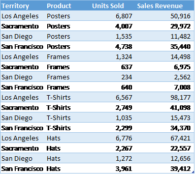
A PivotTable report works best when the source data have:
1. One record in each row;
2. One column for each category for sorting and grouping (such as “Territory” and “Product” in the example above; and
3. One column for each metric (such as “Units Sold” and “Sales Revenue” above). Recording some sales revenue in a different column complicates the task of adding up all of the sales revenue.
Create the PivotTable
Next, create the PivotTable report:
1. Highlight your data table.
2. From the Insert ribbon, click the PivotTable button.
3. On the far right, select fields that you would like on the left-hand side of the report and drag them to the Rows box.
4. Also on the far right, select fields that you would like to appear across the top of the report and drag them to the Columns box.
5. Select the data that you would like to summarize and drag it to the Values box.
6. For each item under Values, specify how to aggregate the data—with a sum, average, or some other function. This is a great time-saving step!
With each change, you’ll see your PivotTable report take shape. If you decide you don’t like the layout, just drag the fields to other positions.
Formatting Your PivotTable Report
From the PivotTable Design ribbon, choose a style for your report based on your theme’s color schemes with options for header rows, header columns, totals, and subtotals. From the Home ribbon, set the number format for your data, or right-click your data, choose Value Field Settings, and click Number Format.
Other Report Options
Do you want even more flexibility in your reports? Do you ever need to, say, connect to data in an external database or create charts based on your reports? All of these options are available with PivotTables!
Or, if you need more flexibility than PivotTables provide, you can:
1. Create a freeform report by adding totals and subtotals directly to your source data,
2. Use the Group and Subtotal options on the new Outline section of the Data ribbon, or
3. If you’re using Excel 2013, use the new Quick Analysis button.
No matter which option you choose, Excel is one of the most flexible reporting tools available today!
PRYOR+ 7-DAYS OF FREE TRAINING
Courses in Customer Service, Excel, HR, Leadership, OSHA and more. No credit card. No commitment. Individuals and teams.
Источник
Create status and trend reports from a work item query
TFS 2017 | TFS 2015 | TFS 2013
One of the quickest ways to generate a custom work tracking report is to use Excel and start with a flat list query. You can generate both status and trend charts. Also, once you’ve built a report, you can manipulate the data further by adding or filtering fields using the PivotTable.
This feature is supported for the following versions and configurations:
- Azure DevOps Server 2020 and earlier versions configured with SQL Server Analysis Services.
- For Azure DevOps Server 2019 and Azure DevOps Server 2020, supports projects that are defined on project collections configured with the On-premises XML process model. If your collection is configured to support the Inheritance process model, you can use Analytics views to filter work items and generate Power BI reports. To learn more, see What are Analytics views? To learn more about process models, see Customize your work tracking experience.
If you want to export work items to Excel, see Bulk add or modify work items with Excel. To get the latest version of the Azure DevOps add-in for Office, install Azure DevOps Office® Integration 2019.
Here’s an example of a status report generated from a flat-list query.

Prerequisites
You can generate these reports only when you work with an on-premises Azure DevOps Server that has been configured with reporting services.
Your deployment needs to be integrated with reporting services. If your on-premises application-tier server hasn’t been configured to support reporting services, you can add that functionality by following the steps provided here: Add reports to a team project.
You must be a member of the TfsWarehouseDataReader security roles. To get added, see Grant permissions to view or create reports in Azure DevOps Server.
A version of Excel that is compatible with your version of Azure DevOps, such as Office 2010 or later version. For a complete list of supported versions, see Azure DevOps client compatibility, Microsoft Office integration. If you don’t have Excel, install it now.
A version of Visual Studio that supports the Team Explorer plugin, such as Visual Studio or Visual Studio Community. You can install Visual Studio from this download site. Team Explorer is free and requires a Windows OS.
To work from Microsoft Excel and use the Team menu, you’ll need to install Azure DevOps Office® Integration 2019.
Create an Excel report from a flat-list query
Use this procedure when you work from the Team Explorer plug-in for Visual Studio.
Create or open a flat-list query that contains the work items that you want to include in the report.
To view queries in Visual Studio 2019 and later versions, you must choose the Tools option Legacy experience (compatibility mode) as described in Set the Work Items experience in Visual Studio 2019.
Choose the fields you want to base reports on and include them in the filter criteria or as a column option. For non-reportable fields, see Q: Which fields are non-reportable?
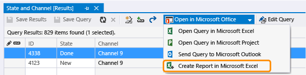
Create a report in Excel From the query results view. The option to Create Report in Microsoft Excel only appears if all prerequisites are met.
Select the check boxes of the reports that you want to generate.
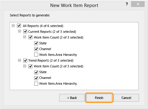
Wait until Excel finishes generating the reports. This step might take several minutes, depending on the number of reports and quantity of data.
Each worksheet displays a report. The first worksheet provides hyperlinks to each report. Pie charts display status reports and area graphs display trend charts.
To view a report, choose a tab, for example, choose the State tab to view the distribution of work items by State.
You can change the chart type and filters. For more information, see Use PivotTables and other business intelligence tools to analyze your data.
Create a query-based report by using Excel
Use this procedure when you work from the web portal or the Team Explorer plug-in for Visual Studio.
Open an Office Excel workbook and choose New Report.
The option New Report appears even if all prerequisites aren’t met. Choosing it may cause Excel to stop responding or display the following error message:


If you don’t see the Team menu, you’ll need to install you’ll need to install the Azure DevOps Office® Integration 2019. See Requirements listed earlier in this article.
Connect to the project and choose the query.
If the server you need isn’t listed, add it now.
Choose the reports to generate (steps 3 and 4 from the previous procedure).
Q: Can I export a query to Excel?
A: If you want to export a query to Excel, you can do that from Excel or Visual Studio/Team Explorer. Or, to export a query directly from the web portal Queries page, install the Azure DevOps Open in Excel Marketplace extension. This extension adds an Open in Excel link to the toolbar of the query results page.
Q: Which fields can’t I use to generate a report?
A: Even though you can include non-reportable fields in your query field criteria or as a column option, they won’t be used to generate a report.
Description, History, and other HTML data-type fields. These fields won’t be added to the PivotTable or used to generate a report. Excel does not support generating reports on these fields.
Fields with filter criteria that specify the Contains, Contains Words, Does Not Contain, or Does Not Contain Words operators will not be added to the PivotTable. Excel does not support these operators. To learn more about these operators, see Query fields, operators, and macros.
Q: Can I create reports if I’m working in Azure DevOps?
A: You can’t create Excel reports; however, you can create query-based charts, generate Power BI reports using an Analytics views, or use the Analytics Service.
Q: How do I refresh the report to show the most recent data?
A: At any time, you can choose Refresh on the Data tab within Excel to update the data for the PivotTables in your workbook. To learn more, see Refresh PivotTable data.
Источник
37
37 people found this article helpful
How to Create a Report in Excel
Using charts, graphs, and pivot tables makes it easy
Updated on September 25, 2022
What to Know
- Create a report using charts: Select Insert > Recommended Charts, then choose the one you want to add to the report sheet.
- Create a report with pivot tables: Select Insert > PivotTable. Select the data range you want to analyze in the Table/Range field.
- Print: Go to File > Print, change the orientation to Landscape, scaling to Fit All Columns on One Page, and select Print Entire Workbook.
This article explains how to create a report in Microsoft Excel using key skills like creating basic charts and tables, creating pivot tables, and printing the report. The information in this article applies to Excel 2019, Excel 2016, Excel 2013, Excel 2010, and Excel for Mac.
Creating Basic Charts and Tables for an Excel Report
Creating reports usually means collecting information and presenting it all in a single sheet that serves as the report sheet for all of the information. These report sheets should be formatted in a way that’s easy to print as well.
One of the most common tools people use in Excel to create reports is the chart and table tools. To create a chart in an Excel report sheet:
-
Select Insert from the menu, and in the charts group, select the type of chart you want to add to the report sheet.
-
In the Chart Design menu, in the Data group, select Select Data.
-
Select the sheet with the data and select all cells containing the data you want to chart (include headers).
-
The chart will update in your report sheet with the data. The headers will be used to populate the labels in the two axis.
-
Repeat the above steps to create new charts and graphs that appropriately represent the data you want to show in your report. When you need to create a new report, you can just paste the new data into the data sheets, and the charts and graphs update automatically.
There are different ways to lay out a report using Excel. You can include graphs and charts on the same page as tabular (numeric) data, or you can create multiple sheets so visual reporting is on one sheet, tabular data is on another sheet, and so on.
Using PivotTables to Generate a Report From an Excel Spreadsheet
Pivot tables are another powerful tool for creating reports in Excel. Pivot tables help with digging more deeply into data.
-
Select the sheet with the data you want to analyze. Select Insert > PivotTable.
-
In the Create PivotTable dialogue, in the Table/Range field, select the range of data you want to analyze. In the Location field, select the first cell of the worksheet where you want the analysis to go. Select OK to finish.
-
This will launch the pivot table creation process in the new sheet. In the PivotTable Fields area, the first field you select will be the reference field.
In this example, this pivot table will show website traffic information by month. So, first, you’d select Month.
-
Next, drag the data fields you want to show data for into the values area of the PivotTable fields pane. You’ll see the data imported from the source sheet into your pivot table.
-
The pivot table collates all of the data for multiple items by adding them (by default). In this example, you can see which months had the most page views. If you want a different analysis, just select the drop-down arrow next to the item in the Values pane, then select Value Field Settings.
-
In the Value Field Settings dialog box, change the calculation type to whichever you prefer.
-
This will update the data in the pivot table accordingly. Using this approach, you can perform any analysis you like on source data, and create pivot charts that display the information in your report in the way you need.
How to Print Your Excel Report
You can generate a printed report from all the sheets you created, but first you need to add page headers.
-
Select Insert > Text > Header & Footer.
-
Type the title for the report page, then format it to use larger than normal text. Repeat this process for each report sheet you plan to print.
-
Next, hide the sheets you don’t want included in the report. To do this, right-click the sheet tab and select Hide.
-
To print your report, select File > Print. Change orientation to Landscape, and scaling to Fit All Columns on One Page.
-
Select Print Entire Workbook. Now when you print your report, only the report sheets you created will print as individual pages.
You can either print your report out on paper, or print it as a PDF and send it out as an email attachment.
FAQ
-
How do I create an expense report in Excel?
Open an Excel spreadsheet, turn off gridlines, and enter your basic expense report information, such as a title, time period, and employee name. Add data columns for Date and Description, and then add columns for expense specifics, such as Hotel, Meals, and Phone. Enter your information and create an Excel table.
-
How do I create a scenario summary report in Excel?
To use Excel’s scenario manager function, select the cells with the information you’re exploring, and then go to the ribbon and select Data. Select What-If Analysis > Scenario Manager. In the Scenario Manager dialog box, select Add. Name the scenario and change your data to see various outcomes.
-
How do I export a Salesforce report to Excel?
In Salesforce, go to Reports and find the report you want to export. Select Export and choose an export view (Formatted Report or Details Only). Formatted Report will export in .xlsx format, while Details Only gives you other choices. Select Export when ready.
Thanks for letting us know!
Get the Latest Tech News Delivered Every Day
Subscribe
Important: In Excel for Microsoft 365 and Excel 2021, Power View is removed on October 12, 2021. As an alternative, you can use the interactive visual experience provided by Power BI Desktop, which you can download for free. You can also easily Import Excel workbooks into Power BI Desktop.
Abstract: This is the third tutorial in a series. In the first tutorial, Import Data into Excel 2013, and Create a Data Model, you created an Excel workbook from scratch using data imported from multiple sources, and its Data Model was created automatically by Excel. The second tutorial,Extend Data Model relationships using Excel 2013, Power Pivot, and DAX, you learned how to extend the Data Model and created hierarchies within the data.
In this tutorial, you use that extended Data Model to build compelling reports that include multiple visualizations using Power View.
The sections in this tutorial are the following:
-
Create a Power View report
-
Create calculated fields for Power View and PivotTables
-
Set field defaults, table behaviors, and data categories
-
Checkpoint and Quiz
At the end of this tutorial is a quiz you can take to test your learning.
This series uses data describing Olympic Medals, hosting countries, and various Olympic sporting events. The tutorials in this series are the following:
-
Import Data into Excel 2013, and Create a Data Model
-
Extend Data Model relationships using Excel 2013, Power Pivot, and DAX
-
Create Map-based Power View Reports
-
Incorporate Internet Data, and Set Power View Report Defaults
-
Power Pivot Help
-
Create Amazing Power View Reports — Part 2
We suggest you go through them in order.
These tutorials use Excel 2013 with Power Pivot enabled. For guidance on enabling Power Pivot, click here.
Create a Power View report
In the previous tutorials, you created an Excel workbook with a PivotTable containing data about Olympic medals and events. If you didn’t complete the previous tutorial, you can download the workbook from the end of the previous tutorial from here.
In this section, you create a Power View report to visually represent the Olympics data.
-
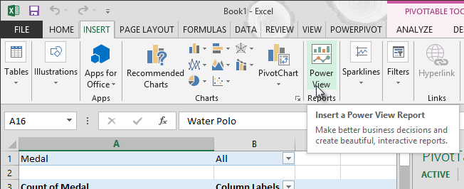
In Excel, click INSERT > Reports > Power View Reports.

-
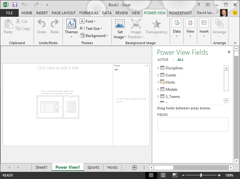
A blank Power View report appears as a sheet in the workbook.
-
In the Power View Fields area, click the arrow beside Hosts to expand it, and click City.
-
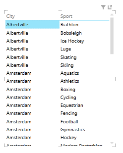
Expand the Medals table, and click Sport. With this, Power View lists the Sport beside the city, as shown in the following screen.
-
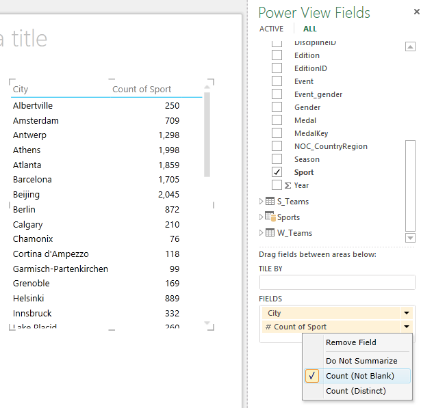
In the FIELDS area of Power View Fields, click the arrow next to Sport and select Count (Not Blank). Now Power View is counting the sports, rather than listing them, as shown in the following screen.
-
On the ribbon, select DESIGN > Switch Visualization > Map. The DESIGN tab is only available if the Power View table is selected. You may get a warning about enabling external content when you switch to the Map visualization.
-
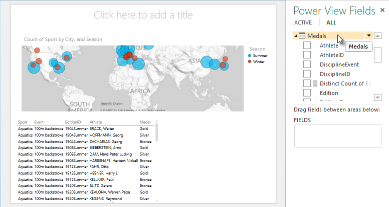
A map replaces the table as the visualization. On the map, blue circles of varying size indicate the number of different sport events held at each Olympic Host location. But it might be more interesting to see which were summer events, and which were winter.
-
To make the most use of the report area, let’s collapse the Filters area. Click the arrow in the upper right corner of the Filters area.
-
In Power View Fields, expand Medals. Drag the Season field down to the COLOR area. That’s better: the map now displays blue bubbles for summer sports, and red bubbles for winter sports, as shown in the following screen. You can resize the visualization by dragging any of its corners.
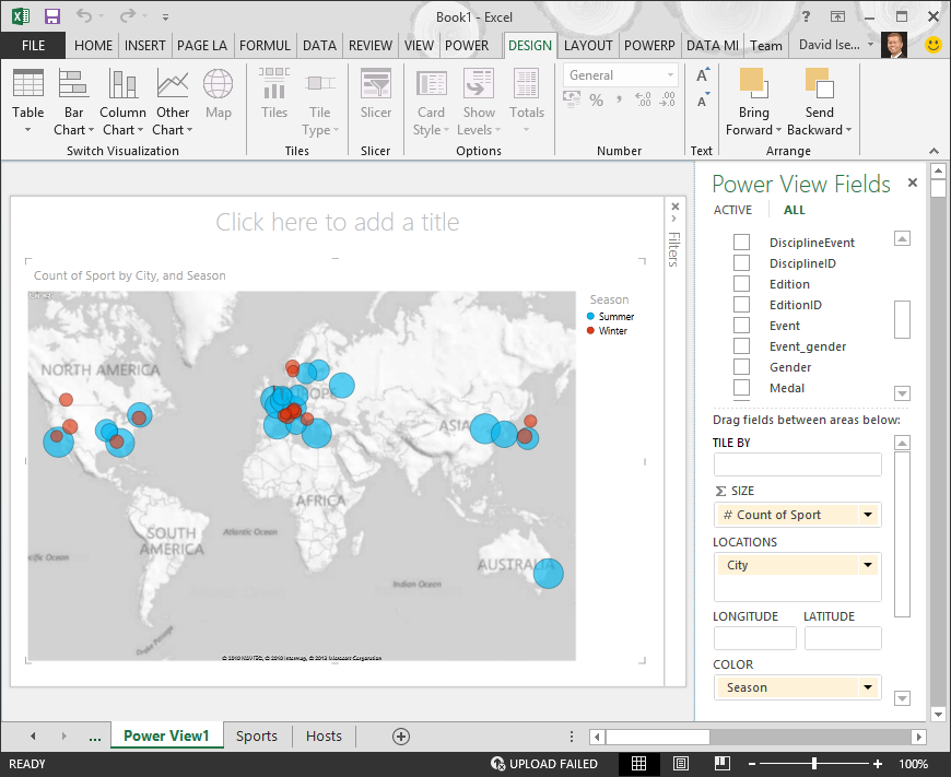
Now you have a Power View report that visualizes the number of sporting events in various locations, using a map, color-coded based on season. And it just took a few clicks.
Create calculated fields for Power View and PivotTables
Power View uses the underlying Data Model to create visualizations. With Power Pivot and DAX, you can extend the Data Model by creating custom formulas, then create reports based on those formulas and calculations in PivotTables and in Power View.
Create a calculated field in
Power Pivot
-
In Excel, click Power Pivot > Data Model > Manage to display the Power Pivot window.
-
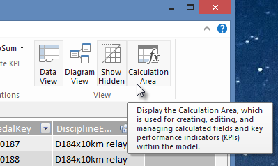
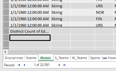
Select the Medals table. Make sure the Calculation Area is displayed. The Calculation Area is found below the table data, and is used for creating, editing, and managing calculated fields. To view the Calculation Area, select Home > View > Calculation Area, as shown in the following screen.
-
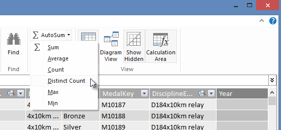
Let’s calculate the number of Olympic editions. In the Calculation Area, select the cell directly below the Edition column. From the ribbon, select AutoSum > Distinct Count, as shown in the following screen.
-
Power Pivot creates a DAX expression for the active cell in the Calculation Area. In this case, Power Pivot automatically created the following DAX formula:
Distinct Count of Edition:=DISTINCTCOUNT([Edition])
Additional calculations in AutoSum are just as easy, such as Sum, Average, Min, Max, and others.
-
Save the Excel workbook. The Data Model is updated with the new calculated field. When you return to the Power View tab in Excel, a warning lets you know the Data Model has been updated, as shown in the following screen.
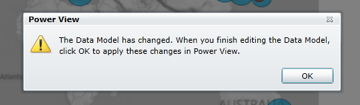
We’ll use this Distinct Count of Edition calculated field later on in the tutorials.
Create a calculated field using DAX in
Power Pivot
The AutoSum calculation is useful, but there are times when more customized calculations are required. You can create DAX formulas in the Calculation Area, just like you create formulas in Excel. Let’s create a DAX formula and then see how it appears in our Data Model, and as a result, is available in our PivotTable and in Power View.
-
Open the Power Pivot window. In the Calculation Area, select the cell directly below the AutoSum calculation you completed in the previous section, as shown in the following screen.
-
Let’s calculate the percentage of all medals. In the formula bar, type the following DAX formula. IntelliSense provides available commands based on what you type, and you can press Tab to select the highlighted IntelliSense option.
Percentage of All Medals:=[Count of Medal]/CALCULATE([Count of Medal],ALL(Medals))
-
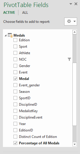
When you switch back to the Excel window, Excel lets you know the Data Model has been updated. In Excel, select the PivotTable in Sheet1. In PivotTable Fields, expand the Medals table. At the bottom of the fields list are the two calculated fields we just created, as shown in the following screen. Select Percentage of All Medals.
-
In the PivotTable, the Percentage of All Medals field appears after Count of Medal. It’s not formatted as a percentage, so select those fields (you can select them all at once, by hovering over the top of one of the Percentage of All Medals field, until the cursor becomes a down arrow, and then clicking). Once they’re selected, click HOME > Number > Percentage. In the same section of the ribbon, adjust the number of decimal places to two. Your pivot table looks like the following screen.
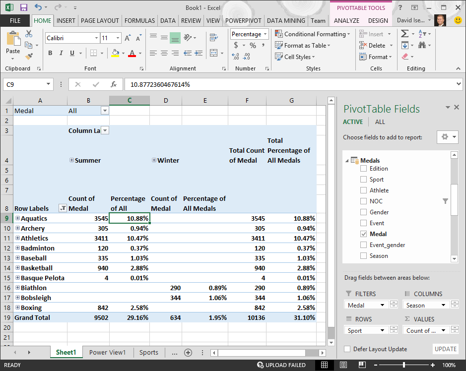
In a previous tutorial, we filtered the Sports field to only the first ten, alphabetically, which is why we only see Aquatics through Boxing, and why the percentage in the Grand Total is 29.16%, rather than 100%. What this does tell us, of course, is that these first ten sports account for 29.16% of all medals awarded in the Summer games. We also can see that Aquatics accounted for 10.88% of all medals.
Since the Percentage of All Medals field is in the Data Model, it’s also available in Power View.
You can also create calculated fields from the Power Pivot tab while in Power View. Whether you create a calculated field in Power Pivot or while in Power View, the result is the same: the Data Model is updated to include the calculated field, and makes it available to all client tools.
Set field defaults, table behaviors, and data categories
Another way to streamline report creation in Power View is by setting a default field set. When you set a default field set for a table, you can simply click that table in Power View, and the default set of fields is automatically added to a new report.
In this section, you set defaults for your workbook that will save you time when creating reports.
Create the Default Field Set for a table
-
The Power Pivot window should still be available. If not, click Power Pivot > Data Model> Manage. In Power Pivot, select Home > View > Data View to make sure Data View is selected. Select the Medals table.
-
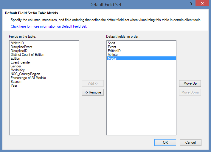
On the Advanced tab, click Reporting Properties > Default Field Set. A window appears that lets you specify default fields for tables created using client tools such as Power View.
-
Select Sport, Event, EditionID, Athlete, and Medal in the left pane, and click Add -> to make them the default fields. Make sure they appear in the right pane, Default fields, in the order they were listed. The Default Field Set window looks like the following screen.
-
Click OK to save the default field set for the Medals table.
-
To see how this works, switch to the Power View sheet in Excel.
-
Click anywhere on the blank report canvas, to make sure you don’t have an existing visualization selected. Your Power View sheet currently only has one visualization, which is the map you created earlier.
-
In the Power View Fields list, click the Medals table name. Power View creates a table and automatically adds the five default fields from the Medals table, in the order you specified, as shown in the following screen. If you accidentally click on the triangle beside Medals, the table simply expands, rather than adding a new table with default fields.
Set Table Behavior
You can also set the default table behavior, which Power View uses to automatically create report labels for the table. This becomes useful when you create visualizations from the same table, perhaps for many different reports. We use default table behavior in the next few steps, so let’s set it now.
-
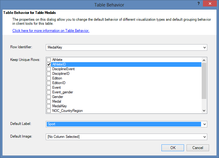
Back in Power Pivot, with the Medals table selected, select Advanced > Reporting Properties > Table Behavior. A window appears where you can specify table behavior.
-
In the Table Behavior window, the Row Identifier is the column that contains only unique keys and no blank values. This is often the table’s primary key, but doesn’t have to be. You have to select a Row Identifier before making other selections in the window. Select MedalKey as the Row Identifier.
-
In the Keep Unique Rows section, select AthleteID. Fields you select here have row values that should be unique, and should not be aggregated when creating Pivot Tables or Power View reports.
Note: If you have trouble with reports that don’t aggregate how you want them to, ensure the field you want to aggregate is not selected in the Keep Unique Rows fields.
-
For Default Label, select a key that should be used as a default report label. Select Sport.
-
For Default Image, leave the selection as [No Column Selected], since you haven’t added images yet. The Table Behavior window looks like the following screen.
-
Click OK. On the Power View sheet in Excel, select the table you created in the previous steps. From the ribbon, select DESIGN > Table > Card. The table you created changes into a collection of Cards; the data is the same, but the visualization of the data has changed. The table now looks like the following screen.
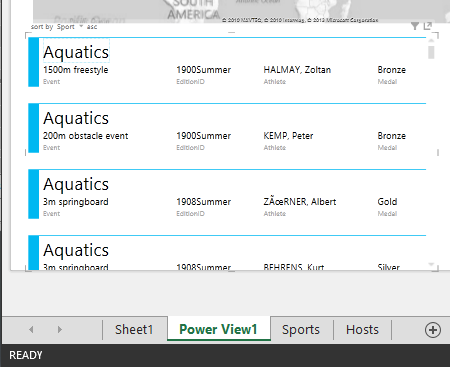
Notice that the Sport field is larger than the rest, and appears as a heading for each card. That’s because you set Sport as the Default Label in the Table Behavior window when you were in Power Pivot.
Set Data Categories for fields
In order for Power View to dynamically create reports based on underlying data, such as location, fields that contain such data must be properly categorized. For the Olympics data, let’s specify the categories for a few fields.
-
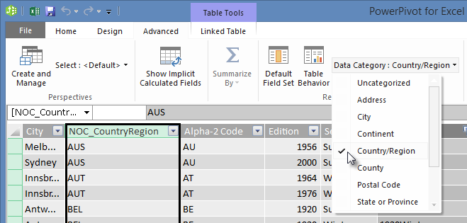
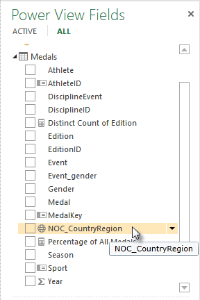
In Power Pivot, select Hosts. Select the NOC_CountryRegion field. From Advanced > Reporting Properties > Data Category: click the arrow and select Country/Region from the list of available data categories, as shown in the following screen.
-
In Medals, select the NOC_CountryRegion column. Again, change the Data Category to Country/Region.
-
Return to Excel, and select the Power View sheet. Expand the Medals table in Power View Fields, and notice that the NOC_CountryRegion field now has a small globe icon beside it. The globe indicates that NOC_CountryRegion contains a geographic location, as shown in the following screen.
We’ll use that geographic location in an upcoming tutorial. It’s time to save your work, review what you’ve learned, and then get ready to dive into the next tutorial.
Checkpoint and Quiz
Review what you learned
In this tutorial you learned how to create a map-based Power View visualization, then created calculated fields to extend your Data Model, and analyze the data in a different way. You also learned how to create default field sets for a table, which streamlined creating a new Power View table pre-populated with the default set of fields. You also learned how to define default table behavior, so the ordering and labeling of new tables was fast and consistent.
In the next tutorial in this series, you build on what you learned here. There’s a lot of data out there, and in the next tutorial, you add Internet data into your Data Model, and bring in images so that your Power View reports can really shine.
Here’s a link to the next tutorial:
Tutorial: Incorporate Internet Data, and Set Power View Report Defaults
QUIZ
Want to see how well you remember what you learned? Here’s your chance. The following quiz highlights features, capabilities, or requirements you learned about in this tutorial. At the bottom of the page, you’ll find the answers. Good luck!
Question 1: Where does Power View get its data to create Power View reports?
A: Only from worksheets included in Excel.
B: Only from the Data Model.
C: Only from data imported from external sources.
D: From the Data Model, and from any data that exists in the worksheets in Excel.
Question 2: Which of the following is true about a default field set?
A: You can only create one default field set for the entire Data Model.
B: In Power View, clicking the table name in Power View Fields creates a table visualization that is automatically populated with the its default field set.
C: If you create a default field set for a table, all other fields in that table are disabled.
D: All of the above
Question 3: Which of the following is true about Calculated Fields?
A: When you create them in Power Pivot, they appear in Power View as fields available in the table in which they were created.
B: If you create them in the Calculation Area of Power Pivot, they are hidden from all client tools.
C: When you create them in Power Pivot, they each appear as individual tables in all client tools.
D: Both A and B.
Question 4: In the Default Behavior Table window, if you select a field in Keep Unique Rows, which of the following is correct?
A: You must explicitly select “Sum this field” from Power View Fields in order to aggregate the field.
B: The field is always aggregated in Power View or PivotTables.
C: The field is never aggregated in Power View or PivotTables.
D: Selecting Keep Unique Rows has no effect on the behavior of the field in Power View or PivotTables.
Quiz an
swers
-
Correct answer: B
-
Correct answer: B
-
Correct answer: A
-
Correct answer: C
Notes:
-
Data and images in this tutorial series are based on the following:
-
Olympics Dataset from Guardian News & Media Ltd.
-
Flag images from CIA Factbook (cia.gov)
-
Population data from The World Bank (worldbank.org)
-
Olympic Sport Pictograms by Thadius856 and Parutakupiu
All the people working in a professional environment understand the need to create a report. It summarizes the whole data of your work or the company’s in a very accurate manner. You can create a report of the data you entered on an Excel Sheet by adding a PivotTable for your entries. A Pivot table is a very useful tool as it calculates the total for your data automatically and helps you analyse your data with different series. You can use a PivotTable to summarize your data and present it to the concerned parties as a report.
Here is how you can make a PivotTable on MS Excel.
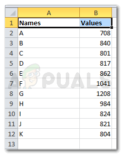
- It is easier to make a report on your Excel sheet when it has the data . After the data has been added, you will have to select the columns or rows you want a PivotTable for.

add the data 
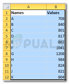
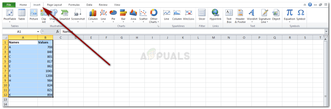
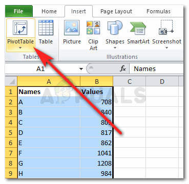
Selecting the rows and columns for your data - Once the data has been selected, go to Insert that is showing on the top tool bar on your Excel software.

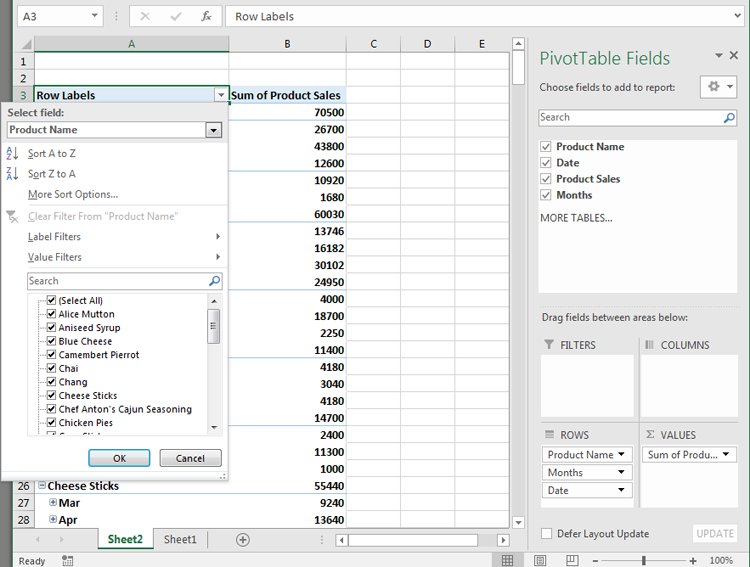
Insert Clicking on Insert will direct you to many options for tables and other important features. On the extreme left, you will find the tab for ‘PivotTable’ with a downward arrow.

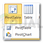
Locate PivotTable on your screen - Clicking on the downward arrow will show you two options to choose from. PivotTable or PivotChart. Now it is up to you and your requirements what you want to make a part of your report. You can try both to see which one looks more professional.

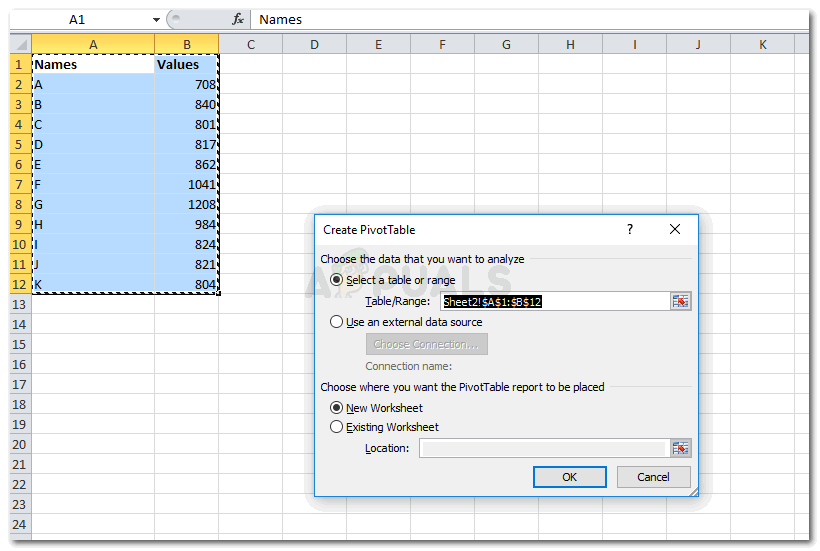
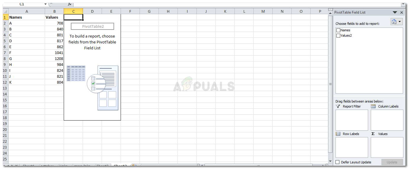
PivotTable to make a report - Clicking on PivotTable will lead you to a dialogue box where you can edit the range of your data, and other choices of whether you want the PivotTable on the same worksheet or you want it on a completely new one. You can also use an external data source if you don’t have any data on your excel. This means, having data on your Excel is not a condition for PivotTable.

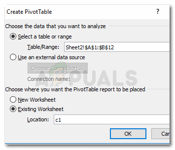
selecting the data and clicking on PivotTable You need to add a location if you want the table to appear on the same worksheet. I wrote c1, you can choose the middle of your sheet as well to keep it all organized.

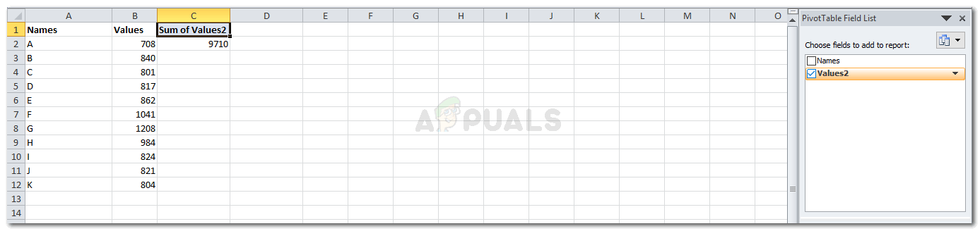
PivotTable: selection of data and location - When you click on OK, your table will not appear as yet. You need to select the fields from the field list provided on the right of your screen just as shown in the picture below.

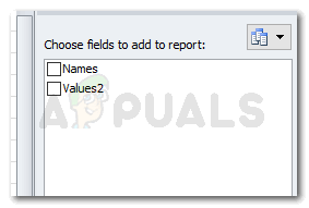
Your report still needs to go through another set of options to finally be made - Check either of the two options for which you want a PivotTable for.

Check the field you want to show on your report You can choose one of them, or both of them. You decide.
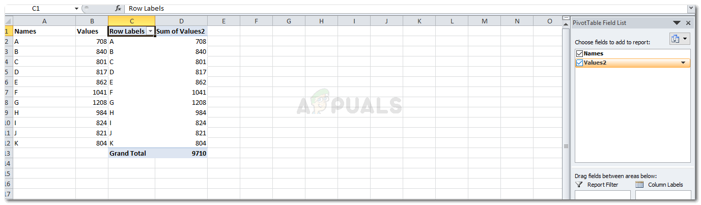
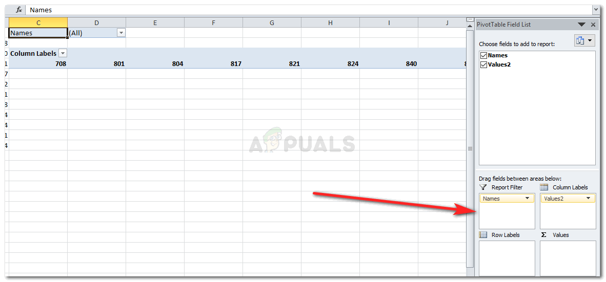
- This is how your PivotTable will look like when you choose both.

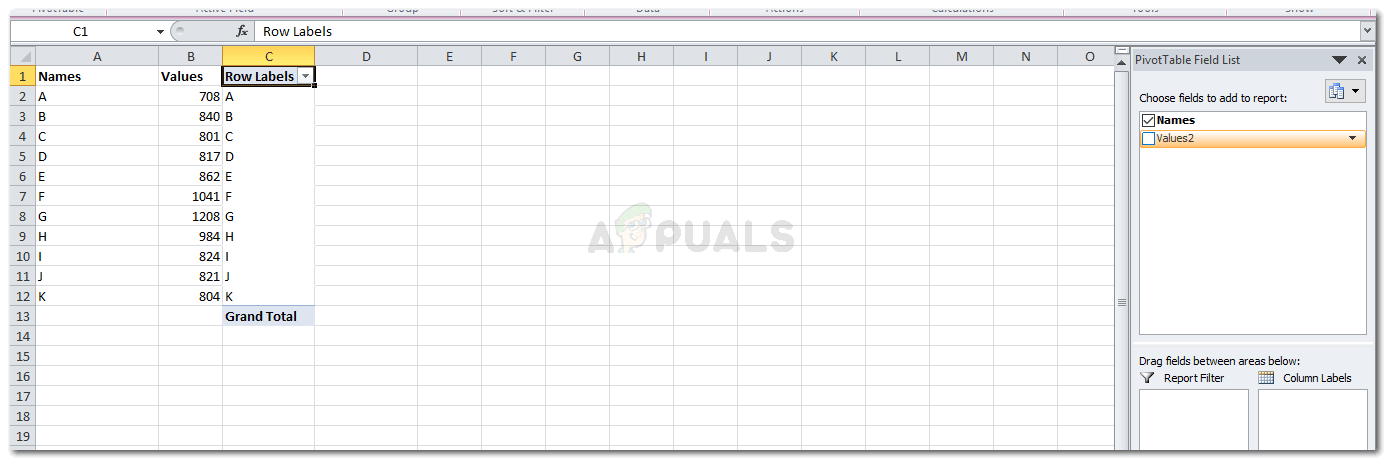
Displaying both the fields And when you select one of the fields, this is how your table will appear.

Displaying one field 
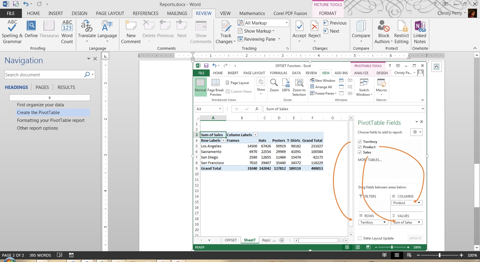
Displaying one field - The option on the right of your screen as shown in the picture below are very important for your report. It helps you make your report even better and more organized. You can drag the columns and rows in between these four spaces to alter the way your report appears.

Important for placement of your report data 
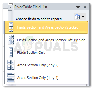
Your report has been made - The following tab on the Field list on your right makes your view of all the fields more easy. You can change it with this icon on the left.

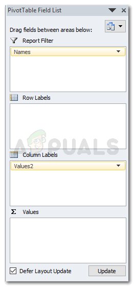
Options for the way your field view looks like. And choosing any of the options from these would change the way your field list shows. I selected ‘Areas Section Only 1 by 4’

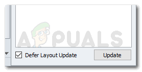
Field List view - Note: The option for ‘Defer Layout Update’ which is right at the end of your PivotTable Field List,is a way of finalizing the fields that you want displaying on your report. When you check the box next to it and click on update, you cannot change anything manually on the excel sheet. You will have to un-check that box to edit anything on the Excel. And even for opening the downward arrow showing on the columns labels cannot be clicked on unless you un-check the Defer Layout Update.

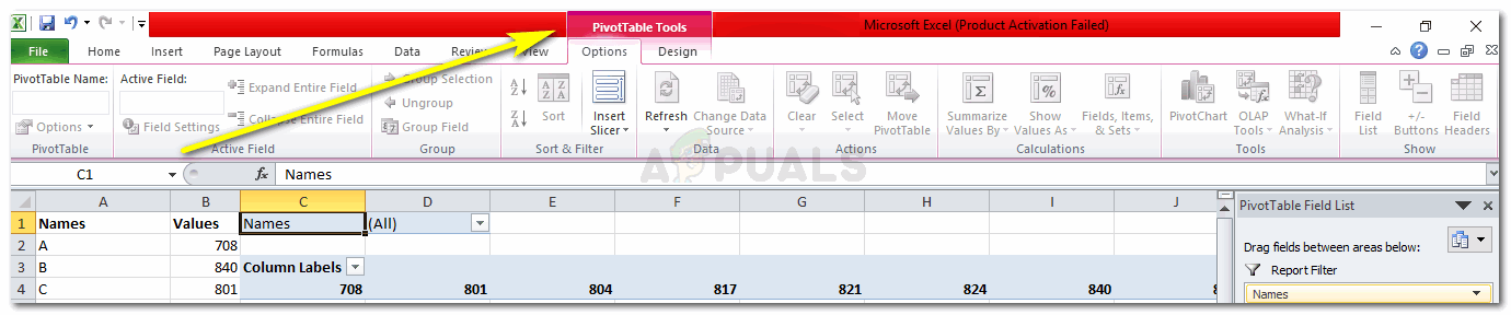
‘Defer Layout Update’, acts more like a lock to keep your edits to the content of the report untouched - Once you are done with your PivotTable, you can now edit it further by using the PivotTable Tools which appear right at the end of all the tools on your tool bar on the top.

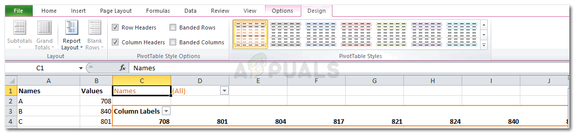
PivotTable Tools for editing how it looks 
All the options for Design


Habiba Rehman
Major love for reading, but writing is what keeps me going. Dream to publish my own novels someday.
Maintenance Alert: Saturday, April 15th, 7:00pm-9:00pm CT. During this time, the shopping cart and information requests will be unavailable.
Categories: Basic Excel
Excel is a powerful reporting tool, providing options for both basic and advanced users. One of the easiest ways to create a report in Excel is by using the PivotTable feature, which allows you to sort, group, and summarize your data simply by dragging and dropping fields.
First, Organize Your Data
Record your data in rows and columns. For example, data for a report on sales by territory and product might look like this:
A PivotTable report works best when the source data have:
1. One record in each row;
2. One column for each category for sorting and grouping (such as “Territory” and “Product” in the example above; and
3. One column for each metric (such as “Units Sold” and “Sales Revenue” above). Recording some sales revenue in a different column complicates the task of adding up all of the sales revenue.
Create the PivotTable
Next, create the PivotTable report:
1. Highlight your data table.
2. From the Insert ribbon, click the PivotTable button.
3. On the far right, select fields that you would like on the left-hand side of the report and drag them to the Rows box.
4. Also on the far right, select fields that you would like to appear across the top of the report and drag them to the Columns box.
5. Select the data that you would like to summarize and drag it to the Values box.
6. For each item under Values, specify how to aggregate the data—with a sum, average, or some other function. This is a great time-saving step!
With each change, you’ll see your PivotTable report take shape. If you decide you don’t like the layout, just drag the fields to other positions.
Formatting Your PivotTable Report
From the PivotTable Design ribbon, choose a style for your report based on your theme’s color schemes with options for header rows, header columns, totals, and subtotals. From the Home ribbon, set the number format for your data, or right-click your data, choose Value Field Settings, and click Number Format.
Other Report Options
Do you want even more flexibility in your reports? Do you ever need to, say, connect to data in an external database or create charts based on your reports? All of these options are available with PivotTables!
Or, if you need more flexibility than PivotTables provide, you can:
1. Create a freeform report by adding totals and subtotals directly to your source data,
2. Use the Group and Subtotal options on the new Outline section of the Data ribbon, or
3. If you’re using Excel 2013, use the new Quick Analysis button.
No matter which option you choose, Excel is one of the most flexible reporting tools available today!
PRYOR+ 7-DAYS OF FREE TRAINING
Courses in Customer Service, Excel, HR, Leadership,
OSHA and more. No credit card. No commitment. Individuals and teams.
![]()
Download Article
![]()
Download Article
This wikiHow teaches you how to automate the reporting of data in Microsoft Excel. For external data, this wikiHow will teach you how to query and create reports from any external data source (MySQL, Postgres, Oracle, etc) from within your worksheet using Excel plugins that link your worksheet to external data sources.
For data already stored in an Excel worksheet, we will use macros to build reports and export them in a variety of file types with the press of one key. Luckily, Excel comes with a built-in step recorder which means you will not have to code the macros yourself.
-
1
If the data you need to report on is already stored, updated, and maintained in Excel, you can automate reporting workflows using Macros. Macros are a built in function that allow you to automate complex and repetitive tasks.
-
2
Open Excel. Double-click (or click if you’re on a Mac) the Excel app icon, which resembles a white «X» on a green background, then click Blank Workbook on the templates page.
- On a Mac, you may have to click File and then click New Blank Workbook in the resulting drop-down menu.
- If you already have an Excel report that you want to automate, you’ll instead double-click the report’s file to open it in Excel.
Advertisement
-
3
Enter your spreadsheet’s data if necessary. If you haven’t added the column labels and numbers for which you want to automate results, do so before proceeding.
-
4
Enable the Developer tab. By default, the Developer tab doesn’t show up at the top of the Excel window. You can enable it by doing the following depending on your operating system:
-
Windows — Click File, click Options, click Customize Ribbon on the left side of the window, check the «Developer» box in the lower-right side of the window (you may first have to scroll down), and click OK.[1]
-
Mac — Click Excel, click Preferences…, click Ribbon & Toolbar, check the «Developer» box in the «Main Tabs» list, and click Save.[2]
-
Windows — Click File, click Options, click Customize Ribbon on the left side of the window, check the «Developer» box in the lower-right side of the window (you may first have to scroll down), and click OK.[1]
-
5
Click Developer. This tab should now be at the top of the Excel window. Doing so brings up a toolbar at the top of the Excel window.
-
6
Click Record Macro. It’s in the toolbar. A pop-up window will appear.
-
7
Enter a name for the macro. In the «Macro name» text box, type in the name for your macro. This will help you identify the macro later.
- For example, if you’re creating a macro that will make a chart out of your available data, you might name it «Chart1» or similar.
-
8
Create a shortcut key combination for the macro. Press the ⇧ Shift key along with another key (e.g., the T key) to create the keyboard shortcut. This is what you’ll use to run your macro later.
- On a Mac, the shortcut key combination will end up being ⌥ Option+⌘ Command and your key (e.g., ⌥ Option+⌘ Command+T).
-
9
Store the macro in the current Excel document. Click the «Store macro in» drop-down box, then click This Workbook to ensure that the macro will be available for anyone who opens the workbook.
- You’ll have to save the Excel file in a special format for the macro to be saved.
-
10
Click OK. It’s at the bottom of the window. Doing so will save your macro settings and place you in record mode. Any steps you take from now until you stop the recording will be recorded.
-
11
Perform the steps that you want to automate. Excel will track every click, keystroke, and formatting option you enter and add them to the macro’s list.
- For example, to select data and create a chart out of it, you would highlight your data, click Insert at the top of the Excel window, click a chart type, click the chart format that you want to use, and edit the chart as needed.
- If you wanted to use the macro to add values from cells A1 through A12, you would click an empty cell, type in =SUM(A1:A12), and press ↵ Enter.
-
12
Click Stop Recording. It’s in the Developer tab’s toolbar. This will stop your recording and save any steps you took during the recording as an individual macro.
-
13
Save your Excel sheet as a macro-enabled file. Click File, click Save As, and change the file format to xlsm instead of xls. You can then enter a file name, select a file location, and click Save.
- If you don’t do this, the macro won’t be saved as part of the spreadsheet, meaning that other people on different computers won’t be able to use your macro if you send the workbook to them.
-
14
Run your macro. Press the key combination which you created as part of the macro to do so. You should see your spreadsheet automate according to your macro’s steps.
- You can also run a macro by clicking Macros in the Developer tab, selecting your macro’s name, and clicking Run.


Advertisement
-
1
Download Kloudio’s Excel plugin from Microsoft AppSource. This will allow you to create a persistent connection between an external database or data source and your workbook. This plugin also works with Google Sheets.
-
2
Create a connection between your worksheet and your external data source by clicking the + button on the Kloudio portal. Type in the details of your database (database type, credentials) and select any security/encryption options if working with confidential or company data.
-
3
Once you’ve created a connection between your worksheet and your database, you will be able to query and build reports from external data without leaving Excel. Create your custom reports from the Kloudio portal and then select them from the drop-down menu in Excel. You can then apply any additional filters and choose the frequency that the report will refresh (so you can have your sales spreadsheet update automatically every week, day, or even hour.)
-
4
In addition, you can also input data into your connected worksheet and have the data update your external data source. Create an upload template from the Kloudio portal and you will be able to manually or automatically upload changes in your spreadsheet to your external data source.


Advertisement
Ask a Question
200 characters left
Include your email address to get a message when this question is answered.
Submit
Advertisement
Video
-
Only download Excel plugins from Microsoft AppSource, unless you trust the third party provider.
-
Macros can be used for anything from simple tasks (e.g., adding values or creating a chart) to complex ones (e.g., calculating your cell’s values, creating a chart from the results, labeling the chart, and printing the result).
-
When opening a spreadsheet with your macro included, you may have to click Enable Content in a yellow banner at the top of the window before you can use the macro.
Thanks for submitting a tip for review!
Advertisement
-
Macros can be used maliciously (e.g., to delete files on your computer). Don’t run macros from untrustworthy sources.
-
Macros will implement literally every step you make while recording. Make sure that you don’t accidentally enter the incorrect value, open a program you don’t want to use, or delete a file.
Advertisement
About This Article
Article SummaryX
1. Enable the Developer tab.
2. Click the Developer tab.
3. Click Record Macro.
4. Create a shortcut key.
5. Store the content in the current workbook.
6. Click OK.
7. Perform the steps you want to automate.
8. Click Stop Recording.
9. Use the shortcut key to run the same steps.
Did this summary help you?
Thanks to all authors for creating a page that has been read 543,765 times.
Is this article up to date?


In Excel 2016, users will find that they have numerous ways of organizing and visualizing their records. Making use of these options will allow you to put tables and charts together to create reports worthy of praise.
- Basic chart and table creation
- How to create PivotTables
- How to create a Dashboard
- Timelines and Slicers
Basic chart and table creation
Before you can impress your team with an in-depth report, you need to learn how to generate charts, tables, and other visual elements. Here are a few types to get you started.
How to create a basic forecast report
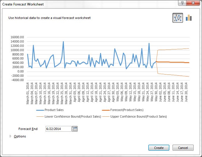
- Load a workbook into Excel
- Select the top-left cell in the source data
- Click on Data tab in the navigation ribbon
- Click on Forecast Sheet under the Forecast section to display the Create Forecast Worksheet dialog box
- Choose between a line graph or bar graph
- Choose Forecast end date
- Click Options for customization
- Select Forecast start date
Forecast reports are useful for calculating projections for sales, growth or revenue.
How to create hierarchal charts
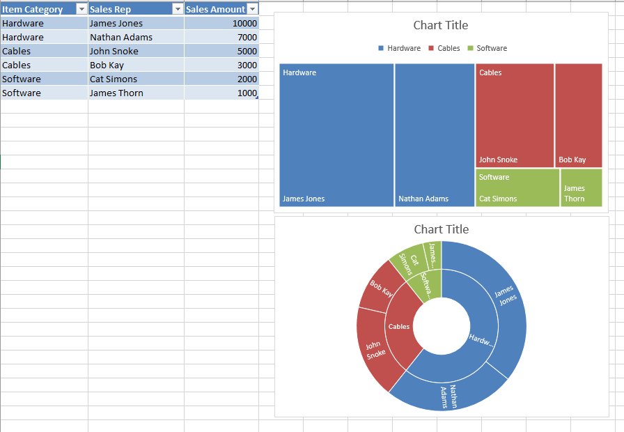
- Select a cell inside of the data table
- Click on Insert in the ribbon
- Click Insert Hierarchy Chart under the Charts group
- Select between TreeMap or Sunburst chart
- Click on the + (plus) sign to add or remove chart elements such as title, data labels, and legend
- Click on the right arrow for each element to customize the appearance or behavior
The Charts group itself is an effective way to find the chart that best suits your data. In fact, Excel 2016 has a Recommended Charts option, which allows you to scroll through shortlisted charts or through all available charts.
How to create PivotTables
A PivotTables enable users to sort through and reorganize data in columns and rows in order to find the most effective view. It’s especially useful when you are working with vast amounts of data.
How to create a recommended P{ivotTable
- Select a cell within the table range or source data
- Navigate to the Tables section in the Insert ribbon tab
- Select Recommended PivotTable
- Browse through the presented types of PivotTables
- Click on the PivotTable you want
- Click OK to generate
- Select Seasonality options
- Modify timeline and value ranges
- Select to fill any missing points by zeros or by interpolation
- Select criteria to aggregate duplicates by
- Select Create to finish
How to create your own PivotTable
- Click on a cell within the source data or table range
- Click on the Insert tab in the navigation ribbon
- Select PivotTable in the Tables section to generate the Create PivotTable dialog box
- Decide on the data source in the Choose the data that you want to analyze section, in case you don’t want to use the selected source
- Select New or Existing Worksheet under the Choose where you want the PivotTable to be placed section
- Click Add this data to the Data Model to incorporate additional data sources in the PivotTable
- Click on fields to include in the report in the PivotTable Fields
- Click and drag fields to reside in either Filters, Columns, Rows, and Values
Once you have decided on the layout and contents of your PivotTable fields, you can use it as the foundation for other Pivot Tables.
How to create a Dashboard
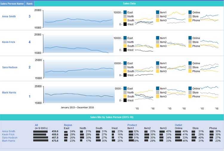
Once you have become comfortable enough to generate charts and tables using your provided data, it’s time to begin piecing the story together in a dashboard. The Dashboard is your chance to showcase your data in an attractive, informative and insightful hub view. It provides a top-level view of the data, allowing your audience to quickly see data and trends in order to view results and make decisions. This reporting tool is highly adaptable and can be used to report a plethora of results regardless of your line of business.
How to prepare your PivotTables for the Dashboard
- Select the original PivotTable that wish to use as your master or reference table
- Right-click on the selection
- Choose Copy
- Select another cell on your worksheet
- Right-click on the selected cell
- Choose Paste to duplicate
- Repeat steps No. 4 to No. 6 as needed
- Click on PivotTable Tools for each table
- Click Analyze
- Insert a name in the PivotTable Name box to identify the function of each table
How to generate PivotCharts from PivotTables
- Select the original PivotTable
- Click on PivotTable Tools
- Select Analyze
- Select PivotChart
- Choose the type of chart that you need
- Choose formatting options in the PivotChart Tools tab
- Click on Analyze under PivotChart Tools
- Enter a name in the Chart Name box
- Apply steps No. 1 to No. 8 as needed for all PivotTables in use
Timelines and Slicers
With your multiple PivotCharts and PivotTables created, you’ll need to be able to find specific information that supports the details you wish to share in the dashboard. Slicers and Timelines provide a way to filter through the data with ease. Timelines allow you to filter by time to locate a specific period. Slicers are essentially click-to-filter options for PivotTables. Not only do they apply a filter, they also indicate the filter currently in use.
How to add a Slicer
- From a PivotTable click on PivotTable Tools
- Select Analyze
- Select Filter
- Select Insert Slicer
- Select the items to be used as slicers
- Click Ok
- Select a Slicer
- Click on Slicer Tools
- Select Options
- Select Report Connections
- Choose the PivotTables that connect to the chosen Slicer
How to add a Timeline
- Click on a PivotTable
- Select Analyze
- Select Filter
- Select Insert Timeline
- Click on the items to use in the Timeline
- Click on the Timeline
- Select Tools
- Select Options
- Select Report Connections
- Select PivotTables to link the Timeline to
With each resulting chart, you can choose to copy and paste it on your dashboard. You can then decide how the dashboard should appear, what will tell the best story for your report.
This results in a dynamic dashboard that allows recipients to look over your presented data while allowing them to sort through the data to give them customization options pertinent to them. If you are creating a Dashboard to be used on a regular basis, you only need to update the source data to recreate the report with new information.
Wrapping Up
There isn’t one report to rule them all, but Excel has the tools to help you make the report you need. How often do you have to create reports in Excel? Which one are you most proud of? Let us know in the comments. And be sure to visit our Office 101 help hub for more related articles!
- Microsoft Office 101: Help, how-tos and tutorials
All the latest news, reviews, and guides for Windows and Xbox diehards.
Most Popular
Excel reports output a downloadable Excel spreadsheet that contains the defined data set and any templates, charts, tables, or other elements added to the customized Excel template. Excel reports use the Report wizard’s filters and groupings/summaries, and once the report parameters have been defined in the rest of the wizard, you can download the Excel template in the Customize Excel tab of the Report wizard and begin to customize it. For example, after defining the data, filters, groupings, and other parameters, you might customize the template to include a PivotTable analyzing the data, and a PivotChart to display the results at a glance.

Unlike graphical, HTML, and text reports, Excel reports can pull data from multiple tables. You can then use PivotTables and charts to analyze the data in any combination. To create an Excel report with data from multiple tables, configure an Excel report in each table with the data you want to use, and then create a combined report that uses those reports as data sources.
Excel reports look different from other reports, so if you haven’t worked with them before, we recommend exploring the Example Reports before you begin.
Example Reports
Before you create your own Excel reports, it can be helpful to explore an example to see how these reports work differently from graphical charts, custom summary reports, or HTML and text reports. In this section, you can follow a guided tour of two example Excel templates.
Single-Source Example
Let’s begin with a simple example template that pulls data from a single source.
- Download Contracts Excel Dashboard.zip, extract the Excel file, and open it.
- Explore the contents of the Sample Dashboard worksheet. This worksheet arranges all the configured charts onto one screen to function as a dashboard.
- Click through the next worksheets, which each contain one of the charts shown on the Sample Dashboard worksheet. In this example, each chart is placed with its corresponding PivotTable on its own worksheet, and duplicated on the Dashboard worksheet. Keeping PivotTables separated can help prevent problems and make maintenance easier.
- Open the last worksheet, titled Data. This worksheet contains the data pulled by the report and placed into the Excel file. The columns are determined by the report’s defined view, and the records included are determined by the report parameters. The charts and PivotTables we explored in steps 2 and 3 refer to this worksheet, so it’s important to preserve the layout and format of the Data worksheet. For example, if someone updated the view for this report and removed the Contract Start Date, several of the charts would break.
To create a similar single-source Excel report, complete the steps in the Create a Basic Excel Report and the Customize the Excel Template sections.
Multi-Source Example
Now, let’s explore a more complex example that pulls data from four sources.
- Download Combined Dashboard.zip, extract the Excel file, and open it.
- Explore the contents of the Dashboard worksheet. This worksheet arranges several charts onto one screen to function as a dashboard.
- Open the next worksheet, Pivot Tables. This example places all the PivotTables onto a single worksheet. These tables are used to create the charts on the Dashboard worksheet. When the template includes several automatically-created Data worksheets, you might find it helpful to concentrate your PivotTables onto a single shared worksheet to make the file easier to navigate.
- Click through the last four worksheets, titled Data1, Data2, Data3, and Data4. Each worksheet contains the data pulled by one of the specified source reports. Each worksheet has its own set of columns defined by the view of the source report, and the records included are determined by the source report parameters. The charts and PivotTables we explored in steps 2 and 3 refer to these worksheets, so it’s important to preserve the layout and format of the Data worksheet, and not to change the order of the source reports after you’ve configured the Excel template.
To create a similar multi-source Excel report, create a basic Excel report for each source table. Then, create a combined report using the basic reports you created, and finally complete the steps to Customize the Excel Template.
Create a Basic Excel Report
In general, report parameters depend heavily on your specific reporting needs. When you set up an Excel report, there are additional considerations for certain parameters.
If you’re planning to create a combined Excel report with data from several tables, you need to configure an Excel report in each table that identifies the data using the steps in this section. Make sure you configure a report in each table you want to include in your final report.
Create a View for the Report
The view you choose for an Excel report determines how the report data is imported and formatted into the Data worksheet of the final file. All your template customization will rely on the column arrangement of the Data worksheet, so it is important to configure the view correctly the first time you set up the report, to avoid accidentally breaking the report.
-
Before you begin, determine the purpose of this view. Specifically, decide whether the view will be used outside of Excel reporting, and whether the view will be used for just this report or for multiple Excel reports.
We recommend creating a view specifically for Excel reports that is not used in the normal table view. If you are comfortable working with Excel, you might be able to create one view to use in all Excel reports for the table; this requires including more data than you need for any individual report and combing through the data in Excel later. If you are less comfortable working with lots of data in Excel, or if your system has an unusually large amount of data, you should consider creating individual views for each Excel report you create.
- Either from the Grouping/Summary tab in the Report wizard or from the table you are reporting on, create a new view.

- If you plan to use this view only for Excel reports, clear the check boxes for selection, edit, and view icons. In Excel, these icons don’t do anything.
- Set Max lines per record and Max lines per linked field to all. This makes sure the complete value is sent to Excel.
- Check the Display check box for the appropriate fields, with the following considerations:
- If you aren’t sure whether you need a field, it’s better to include it. You can always ignore the data in Excel, but it’s difficult to add fields to the view after you create an Excel report.
- If you plan to use this view for other Excel reports, select every field you might need in any of those reports. If you don’t select a field, your Excel reports will not receive any data for that field.
- Always include the ID field and, if possible, a second field with unique values, such as the summary field.
- Go to the Order/Colors tab and configure the field order. This corresponds to the order of the columns in the Excel data worksheet. We recommend putting the ID field and other important fields on the left, just like you do for regular views.
- If you plan to use this view outside of Excel, configure row coloring or notification icons as desired. If you plan to use this view only for Excel reports, you can configure row coloring directly in Excel later.
- Go to the General tab and name the view. Include «DO NOT EDIT» in the name to help prevent users from accidentally editing the view and breaking the report. If you plan to use this view only for Excel reports or only for a specific Excel report, mention that in the name as well.
- Set the Maximum View Width to a high value, such as 900 characters. You can adjust the column width in Excel later.
- Set the Records Per Page to the highest value available.
- Go to the Apply tab and make the view visible to every group that needs to view or edit the Excel report.

Set Up the Report
With your view ready to go, set up your Excel report as desired, with the following options:
- If you’re using this report to create a combined report, on the General tab, make sure the report title mentions the table name. For example, you might name your report «Service Requests Data for Combined Dashboard».
- On the Filter tab, leave the saved search set to None. Results can be filtered using a PivotTable in Excel, so usually a saved search filter isn’t necessary.
- On the Grouping/Summary tab, select the view you created and set a high value in Show not more than X records in each grouping, such as 100,000. This determines how many records are sent to Excel.
- If you aren’t using this report to create a combined report, when you reach the Customize Excel tab, click Create/Download New Excel File and proceed to the Customize the Excel Template section. If you’re using this report to create a combined report, you can skip the customized template.
Combined Reports
If you’re creating a combined Excel report with data from many tables, the first step is creating individual Excel reports in each table you’ll use as a data source. For example, if your combined report includes data from the Service Requests, Incidents, Problems, and Change Requests tables, you need to create an Excel report in each of those tables to identify the data set you want to use. For more guidance on creating usable Excel reports, refer to the Excel Report Parameters section.
After you create all the necessary source reports, your next step is creating a combined report that pulls from the other reports you created.
- In the left pane, expand the Home section and click Summary/combined reports.
- Click New.
- Give your report a title and description. Make sure the description lists the tables you’re using to provide source data.
- Select the Excel output format.
- Go to the Select Reports tab and click New.
- In the Combined Report wizard, select the table and then select the Excel report you created. Click Finish.
-
Repeat step 6 for each table and Excel report you want to include. Each one you select will create a separate Data worksheet in the Excel file.
The reports are sent to the Excel template in the same order they’re listed here. If you want to change the order, click and drag to move the reports.
- Go to the Customize Excel tab.
- Click Create/Download New Excel File and proceed to the Customize the Excel Template section.
- When you finish your Excel template, configure the Schedule and Apply tabs as needed. For details, see Create and Edit Charts and Reports.
Customize the Excel Template
After you configure the first set of report parameters, you need to create a template the system will use to generate your Excel reports. When a report is generated, your template is replicated exactly with the exception of the Data worksheet. The Data worksheet is replaced with new data from the system, pulled in using the parameters and view you configured. The rest of your template is automatically refreshed so the new data is applied.
This section includes tips for working in Excel, but some functionality might be slightly different depending on the version of Excel you are using. For additional help working with Excel, or for information about more advanced Excel features, refer to Microsoft Office support.
- In the Customize Excel tab, click Create/Download New Excel File to download the report with the current parameters.
- If necessary, customize the column width and text wrapping on the Data worksheets to make them readable.
Important: Do not rename Data, Data1, Data2, or similarly named worksheets. The system uses these worksheet names to generate the report correctly. - Add any necessary customization to create your report.
- Create new worksheets for your tables, charts, and dashboards as needed
-
Create PivotTables and PivotCharts on the new worksheets
- Set the design and colors appropriately
- Arrange charts and tables to make the report easy to use
- Save the file.
- Click Choose File and select the Excel report.
- Click Upload Customized Excel File.
- Test the report thoroughly and make adjustments as needed.
- When the report is next run according to the schedule, the system will take the run-time data and apply it to the new Excel report template.
This approach provides a high level of customization using advanced Excel features such as pivot tables, which allow you to segregate a lot of different data into easy views for granular analysis. In this case,
Agiloft simply provides the report data, and the template handles all of the presentation and formatting requirements. This requires the person building the template to have familiarity with advanced Excel functions.
Detailed Excel Customization Example
If you haven’t worked with Excel in the past, you can use this section to learn how to make a basic Excel report using your data. Note that this section assumes you have already completed the steps in
Agiloft to determine your report parameters and specify what data to pull from the system.
Note that the steps refer to the Data worksheet, but if you are working on a combined report, you will have multiple Data worksheets that the steps apply to.
- In the Customize Excel tab, click Create/Download New Excel File to download the report with the current parameters.
- On the Data worksheet, see how your report looks. The Data worksheet is overwritten each time the report is run, so we won’t spend much time on customization here, but you can adjust the column width and turn Wrap Text on or off. For example, if your Data worksheet includes a working notes field with lots of text, you might want to turn Wrap Text on for that column to make the text readable, or turn Wrap Text off and make the column narrow if you don’t intend for anyone to read the text in those fields.
- When you’re satisfied with your Data worksheet formatting, go to Insert > PivotTable.
- Make sure the New Worksheet option is selected and click OK.
- To keep our report tidy, double-click the Sheet1 worksheet at the bottom and rename it PivotTables.
-
Review the PivotTable Fields list and drag some fields into the rows, columns, and values boxes. You can use the drop-down arrow to see additional analysis options for the field, and you can create nested fields by dragging additional fields on top of fields you already added. Experiment with the options until you are satisfied with your table.
If you’ve never created a PivotTable before, start by dragging the ID field into the Values box. Click the drop-down arrow in the box and select Value Field Settings, then change the selection from Sum to Count and click OK. Now, drag another field, such as Status or Priority, into the Rows box. Finally, drag a third field, such as Assigned Team or Department, into the Filters box. This will give you a basic table to use for this exercise.
Now that you’ve created a table, you can create slicers. Slicers make it easy to filter the data without changing the configuration of the PivotTable. Later, we’ll put the slicers on the dashboard next to the corresponding PivotChart, so we can use our dashboard without looking at the PivotTable at all.
- Select a cell inside the PivotTable and go to Analyze > Insert Slicer. Slicers make it easy to filter data directly in the PivotChart we will create from the table, without having to filter the data out of the report entirely or having to narrow your report parameters too closely. For example, you might want to be able to see the number of tickets for a specific team; with a slicer, you can switch between different teams easily, without removing any data from your report.
- If you added a field to the Filters box, select that field for your filter. Otherwise, choose a field such as Assigned Team or Department.
- Click OK.
- With the slicer selected, open the Options ribbon and select a color for this filter. Use the same color for the same type of filter consistently in your report so that your report is easier to read. For example, if you set a Priority slicer to dark blue, you should use the same color for Priority slicers in other tables, and not use dark blue for any other slicers.
- Right-click inside the PivotTable and click PivotTable Options.
- Give the table a clear, descriptive name to differentiate it from other PivotTables you might create later.
- Clear the «Autofit column widths on update» check box. This prevents the column widths from changing unexpectedly when you run the report.
- Click OK.
- Now that the PivotTable is set up, select a cell in the table and open the Design ribbon. Explore the options to change the presentation of the table. For example, change the Report Layout to Tabular Form and see what changes. Play around with these settings to find the best design for your report.
With the PivotTable finalized, it’s time to create a chart and build our dashboard.
- Go to Analyze > PivotChart. Select one of the simple charts, such as a basic bar or line graph, and click OK.
- We want to show our chart on a dashboard, not the PivotTable worksheet. Right-click the worksheet farthest on the left and click Insert. Click OK to add a worksheet, double-click the new worksheet, and rename it Dashboard.
- Go back to the PivotTables worksheet. Right-click the chart and click Cut.
- Go back to the Dashboard worksheet and Paste the chart.
- Cut the slicer from the PivotTables worksheet and Paste it on the Dashboard worksheet.
- Arrange the chart and the slicer together on the page.
The dashboard is starting to come together. Now, clean up the look of the chart:
- Right-click the field buttons in the upper-left corner and click Hide All Field Buttons on Chart.
- Open the Design ribbon and select a default chart design.
- Right-click a data point on the chart and click Format Data Series. Open the paint bucket tab, expand the Fill options, and select the Vary colors by point check box.
- Open the Design ribbon and click Add Chart Element to add or remove any chart element as needed. For example, if the axis labels and the legend show the same information, you could change the Legend element to None.
- Adjust the format of the chart as needed by right-clicking the element you want to change and opening the options for that element.
Finally, clean up the dashboard:
- Select a cell outside the chart and slicer.
- Open the View ribbon and clear the Gridlines check box.
- Open the Home ribbon and use the paint bucket tool to fill in the background with a contrasting color, like dark gray.
Now, you have a basic Excel report with a dashboard and a worksheet for PivotTables. You can add new tables and charts to your report using the same steps as above.
If you add more than one PivotTable in the same worksheet, place the tables in a row horizontally rather than stacking them vertically. If you run the report and a lot of data is found, the tables might become much longer than you expected, and if they are placed in a column, upper tables will overwrite lower tables and break them.
Related articles
Do you want to know how to analyze data in excel?
Are you looking for the best way to analyze data in excel?
Keep Reading!
Microsoft Excel is one of the most widely used tools in any industry. While some enjoy playing with pivotal tables and histograms, others limit themselves to simple pie-charts and conditional formatting.
Some may create an artwork out of the dull monochrome Excel, while others may be satisfied with its data analysis. In this discussion, we will make a deep delving analysis of Microsoft Excel and its utility. We will focus on how to analyze data in Excel Analytics, the various tricks, and techniques for it. The discussion will also explore the various ways to analyze data in Excel.
We will discuss the different features of Excel analytics to know how to analyze data in excel (much of which are unexplored to the mass), functions, and best practices.
Our discussion will include, but not be limited to:
(i) Best Way to Analyze Data in Excel
(ii) How to Analyze Sales Data in Excel
(iii) Analyzing Data Sets with Excel
(iv) Data Segregation with Excel
(v) The Importance of Data Reporting
(vi) How to Analyze Data in Excel

Register For a Free Webinar
Date: 15th Apr, 2023 (Saturday)
Time: 11:00 AM to 12:00 PM (IST/GMT +5:30)
How to Analyze Sales Data in Excel: Make Pivot Table your Best Friend
A pivot tool helps us summarize huge amounts of data. One of the best ways to analyze data in excel, it is mostly used to understand and recognize patterns in the data set.
Recognizing patterns in a small dataset is pretty simple. But the enormity of the datasets often calls for additional efforts to find the patterns. In such cases, a pivot table can be a huge advantage as it takes only a few minutes to summarize groups of data using a pivot table.
A data analysis example can be, you have a dataset consisting of regions and number of sales. You may want to know the number of sales based on the regions, which can be used to determine why a region is lacking and how to possibly improve in that area. Using a pivot table, you can create a report in excel within a few minutes and save it for future analysis.
A Pivot Table allows you to summarize data as averages, sums, or counts in Excel from data that is stored in another Spreadsheet, or table. It is great for quickly building reports because you can sort and visualize the data quickly.
Taking a data analysis example like, you may have put together a spreadsheet, which you can copy, and paste into Excel, or use in Google Docs if you would prefer (just click File > Make a Copy).
The spreadsheet contains data with a mock company’s customer purchase information. Since companies purchase at different dates, a pivot table will help us to consolidate this data to allow us to see total buys per company, as well as to compare purchases across companies, for quick analysis.
The Pivot table allows you to take a table with a lot of data in it and rearrange the table so that you only look at only what matters to you.
- a) Whether you are using a Mac or a PC, you can select the whole dataset that you want to look at and select: “Data” -> “Pivot Table”. When you hit that, a new tab should be opened with a table.
Data Set
- b) Once you have your table in front of you, you can drag and drop the Column Labels, Row Labels, and Report Filter
- Column Labels go across the top row of your table (for example Date, Month, Company Name)
- Row Labels go across the left-hand side of your table [for example Date, Month, Company Name (same as with column labels, it depends on how you would prefer to look at the data, vertically or horizontally)]
- The Values section is where you put the data you would like calculated (for example Purchases, Revenue)
- Report Filter helps you refine your results. Add anything you would like to Filter by (for example you want to look at Lead Referral Sources, but exclude Google and Direct)
Pivot tables are a great way to manage the data from your reports. You can copy and paste the data into your own Excel file, or create a copy in Google Apps (File > Make a Copy).

How to Analyze Data in Excel: Analyzing Data Sets with Excel
To know how to analyze data in excel, you can instantly create different types of charts, including line and column charts, or add miniature graphs. You can also apply a table style, create PivotTables, quickly insert totals, and apply conditional formatting. Analyzing large data sets with Excel makes work easier if you follow a few simple rules:
- Select the cells that contain the data you want to analyze.
- Click the Quick Analysis button image button that appears to the bottom right of your selected data (or press CRTL + Q).
- Selected data with Quick Analysis Lens button visible
- In the Quick Analysis gallery, select a tab you want. For example, choose Charts to see your data in a chart.
- Pick an option, or just point to each one to see a preview.
- You might notice that the options you can choose are not always the same. That is often because the options change based on the type of data you have selected in your workbook.

To understand the best way to analyze data in excel, you might want to know which analysis option is suitable for you. Here we offer you a basic overview of some of the best options to choose from.
- Formatting: Formatting lets you highlight parts of your data by adding things like data bars and colors. This lets you quickly see high and low values, among other things.
- Charts: Charts Excel recommends different charts, based on the type of data you have selected. If you do not see the chart you want, click More Charts.
- Totals: Totals let you calculate the numbers in columns and rows. For example, Running Total inserts a total that grows as you add items to your data. Click the little black arrows on the right and left to see additional options.
- Tables: Tables make it easy to filter and sort your data. If you do not see the table style you want, click More.
- Sparklines: Sparklines are like tiny graphs that you can show alongside your data. They provide a quick way to see trends.

Ways to Analyze Data in Excel: Tips and Tricks
It is fun to analyze data in MS Excel if you play it right. Here, we offer some quick hacks so that you know how to analyze data in excel.
-
How to Analyze Data in Excel: Data Cleaning
Data Cleaning, one of the very basic excel functions, becomes simpler with a few tips and tricks. You may learn how to use a native Excel feature and how to accomplish the same goal with Power Query. Power Query is a built-in feature in Excel 2016 and an Add-in for Excel 2010/2013. It helps you to extract, transform, and load your data with just a few clicks.
1. Change the format of numbers from text to numeric
Sometimes when you import data from an external source other than Excel, numbers are imported as text. Excel will alert you by showing a green tooltip in the top-left corner of the cell.
Depending on the number of values in the range, you can quickly convert the values to numbers by clicking on ‘Convert to a number’ within the tooltip options.
However, if you have more than 1000 values, you will have to wait a couple of seconds while Excel finishes the conversion.
You may also convert the values to number format is to use Text-to-Columns using the following steps:
- Select the range with the values to be converted.
- Go to Data > Text to Columns.
- Select Delimited and click Next.
- Uncheck all the checkboxes for delimiters (see below) and click Next.
- Text-Columns-Checkboxes
2. Select General and click on Finish
When you have lots of numbers to convert this tip will be much faster than waiting for all the numbers to be converted. In Power Query, you just have to right-click on the column header of the column you want to convert.
- Then go to Change Type.
- Then select the type of number you want (such as Decimal or Whole Number)
- Power-Query-Data-Type
Register For a Free Webinar
Date: 15th Apr, 2023 (Saturday)
Time: 11:00 AM to 12:00 PM (IST/GMT +5:30)
How to Analyze Data in Excel: Data Analysis
Data Analysis is simpler and faster with Excel analytics. Here, we offer some tips for work:
- Create auto expandable ranges with Excel tables: One of the most underused features of MS Excel is Excel Tables. Excel Tables have wonderful properties that allow you to work more efficiently. Some of these features include:
- Formula Auto Fill: Once you enter a formula in a table it will be automatically be copied to the rest of the table.
- Auto Expansion: New items typed below or at the right of the table become part of the table.
- Visible headers: Regardless of your position within the table, your headers will always be visible.
- Automatic Total Row: To calculate the total of a row, you just have to select the desired formula.
- Use Excel Tables as part of a formula: Like in dropdown lists, if you have a formula that depends on a Table, when you add new items to the Table, the reference in the formula will be automatically updated.
- Use Excel Tables as a source for a chart: Charts will be updated automatically as well if you use an Excel Table as a source. As you can see, Excel Tables allow you to create data sources that do not have to be updated when new data is included.
How to Analyze Data in Excel: Data Visualization
Quickly visualize trends with sparklines: Sparklines are a visualization feature of MS Excel that allows you to quickly visualize the overall trend of a set of values. Sparklines are mini-graphs located inside of cells. You may want to visualize the overall trend of monthly sales by a group of salesmen.
To create the sparklines, follow these steps below:
- Select the range that contains the data that you will plot (This step is recommended but not required, you can select the data range later).
- Go to Insert > Sparklines > Select the type of sparkline you want (Line, Column, or Win/Loss). For this specific example, I will choose Lines.
- Click on the range selection button Select Range Excel Button to browse for the location of the sparklines, press Enter and click OK. Make sure you select a location that is proportional to the data source. For example, if the data source range contains 6 rows then the location of the sparkline must contain 6 rows.
To format the sparkline you may try the following:
To change the colour of markers:
- Click on any cell within the sparkline to show the Sparkline Tools menu.
- In the Sparkline tools menu, go to Marker Color and change the colour for the specific markers you want.
For example High points on the green, Low points on red, and the remaining in blue.
To change the width of the lines:
- Click on any cell within the sparkline to show the Sparkline Tools menu.
- In the Sparkline tools contextual menu, go to Sparkline Color > Weight and change the width of the line as you desire.
Save Time with Quick Analysis: One of the major improvements introduced back in Excel 2013 was the Quick Analysis feature. This feature allows you to quickly create graphs, sparklines, PivotTables, PivotCharts, and summary functions by just clicking on a button.
When you select data in Excel 2013 or later, you will see the Quick Analysis button Quick Analysis Excel Button in the bottom-right corner of the range selected. If you click on the Quick Analysis button you will see the following options:
- Formatting
- Charts
- Totals
- Tables
- Sparklines
When you click on any of the options, Excel will show a preview of the possible results you could obtain given the data you selected.
- If you click on the Quick Analysis button and go to charts, you could quickly create the graph below just by clicking a button.
- If you go to Totals, you can quickly insert a row with the average for each column:
- If you click on Sparklines, you can quickly insert Sparklines:
- As you can see, the Quick Analysis feature really allows you to quickly perform different visualizations and analysis with almost no effort.
How to Analyze Data in Excel: Data reporting
Data reporting in Excel analytics requires more than just accounting skills, it also requires a thorough knowledge of excel functionalities and the ability to add beauty to your report.
- Turn Auto Refresh off before editing the Excel workbook. This will stop the table from refreshing when you are making changes on the worksheet. To do this, click on the Refresh icon at the bottom of the Excel Report Designer Task Pane and then select “Switch auto-refresh off”.
- When adding a new row to the layout, select a cell in the table area below where you want to insert the new row. Then right-click and from the context menu select Insert > Table Rows Above.
- When deleting columns or rows make sure you use the Table Delete functions similar to the Insert functions above. To remove a column or row, select a cell in the table area of the row or column you want to remove. Then right-click and from the context menu select Delete and then either Table Columns or Table Rows.
- Remove unneeded rows or columns from the table. Having fewer cells in the layout makes it easier for the table to refresh, so removing any unneeded ones will improve performance.

Excel has several other uses that may not have been covered here. Play around with visualize complex data or organize disparate numbers, to discover the infinite variety of functions in Excel analytics. Strong knowledge of excel is a boon if you are looking forward to a career in data analytics.
Register For a Free Webinar
Date: 15th Apr, 2023 (Saturday)
Time: 11:00 AM to 12:00 PM (IST/GMT +5:30)
This was all about how to analyze data in excel, how to analyze sales data in excel along with a few data analysis example.
Hopefully, you must have understood the best way to analyze data in excel.
We offer one of the best-known courses in Data Analytics Using Excel Course. The course enables you to learn tools such as Advanced Excel, PowerBI, and SQL. The live projects and intensive training program also empower you to come up with solutions for real-life problems.