
Create and format tables
Create and format a table to visually group and analyze data.
Note: Excel tables shouldn’t be confused with the data tables that are part of a suite of What-If Analysis commands (Forecast, on the Data tab). See Introduction to What-If Analysis for more information.

Try it!
-
Select a cell within your data.
-
Select Home > Format as Table.
-
Choose a style for your table.
-
In the Create Table dialog box, set your cell range.
-
Mark if your table has headers.
-
Select OK.
-
Insert a table in your spreadsheet. See Overview of Excel tables for more information.
-
Select a cell within your data.
-
Select Home > Format as Table.
-
Choose a style for your table.
-
In the Create Table dialog box, set your cell range.
-
Mark if your table has headers.
-
Select OK.
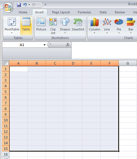
To add a blank table, select the cells you want included in the table and click Insert > Table.
To format existing data as a table by using the default table style, do this:
-
Select the cells containing the data.
-
Click Home > Table > Format as Table.
-
If you don’t check the My table has headers box, Excel for the web adds headers with default names like Column1 and Column2 above the data. To rename a default header, double-click it and type a new name.
Note: You can’t change the default table formatting in Excel for the web.
Want more?
Overview of Excel tables
Video: Create and format an Excel table
Total the data in an Excel table
Format an Excel table
Resize a table by adding or removing rows and columns
Filter data in a range or table
Convert a table to a range
Using structured references with Excel tables
Excel table compatibility issues
Export an Excel table to SharePoint
Need more help?
Try it!
You can create and format a table, to visually group and analyze data.
-
Select a cell within your data.
-
Select Home > Format as Table.
-
Choose a style for your table.
-
In the Format as Table dialog box, set your cell range.
-
Mark if your table has headers.
-
Select OK.
Want more?
Create or delete an Excel table
Need more help?
Want more options?
Explore subscription benefits, browse training courses, learn how to secure your device, and more.
Communities help you ask and answer questions, give feedback, and hear from experts with rich knowledge.
Microsoft Excel is convenient for creating tables and doing calculations. Its working area is a set of cells to be filled with data. Consequently, the data can be formatted, used for building graphs, charts, summary reports.
For a beginner, working with tables in Excel may seem complicated at the first glance. It is differs considerably from the principles of table construction in Word. However, let us start from the very basics: creating and formatting tables. By the time you reach the end of this article, you will understand there is no better tool for creating tables than Excel.
Creating a table in Excel: a dummy’s guide
Working with Excel tables for dummies does not tolerate haste. There are different ways to create a table for a specific purpose, and each of them has its advantages. Therefore, let us start with assessing the situation visually.
Look carefully at the work sheet of the table processor:
It is a set of cells in columns and rows. Essentially, it’s a table. The columns are marked with letters. The rows are designated with numbers. There are no borders.
First of all, let’s learn to work with cells, rows and columns.
How to select a column and a row
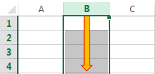
To select the entire column, left-click on the letter that marks it.
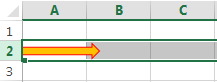
To select a row, click on the number it’s designated with.
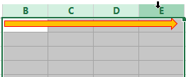
To select several columns or rows, left-click on the name, hold down the button and drag the pointer.
To select a column with the help of hot keys, place the cursor in any cell of the column and press Ctrl + Space. The key combination Shift + Space is used to select a row.
How to resize cells
If your information does not fit in the table, you need to resize the cells.
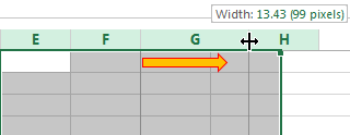
- You can move them manually by grabbing the cell boundary with the left mouse button.
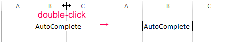
- If the cell contains a long word, you can double-click on the boundary of the column/row. The program will expand its boundary automatically.
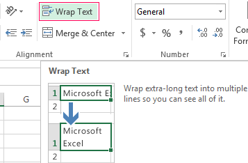
- If you need to increase the height of a row preserving the column width, use the button «Wrap Text» in the tool bar.
To change the column width and the row height in a certain range, resize 1 column/row (by dragging its boundaries manually) – and all the selected columns and rows will be resized automatically.
Important note. To go back to the previous size, you can press the «Undo Typing» button or the hot-key combination CTRL+Z. However, it works only if used immediately. Later on, it will not help.
To bring the rows to their initial boundaries, open the tool menu: «HOME»-«Format» and choose «AutoFit Row Height».
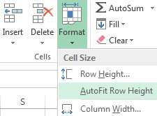
This method does not work for columns. Click «Format» — « AutoFit Row Width» Memorize this number. Select any cell in the column that needs to go back to the initial size. Click «Format» — «Column Width» again and enter the value suggested by the program (as a rule, it’s 8.43 – the number of characters in the Calibri font, size 11 pt). OK.
How to insert a column or row
Select the column/row to the right of/below the place where the insertion needs to be made. That is, the new column will appear to the left of the selected cell. The new row will be pasted above it.
Right-click on the cell and select «Insert» in the drop-down menu (or hit the hot-key combination CTRL+SHIFT+»=»).
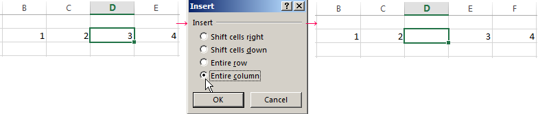
Select «Entire column» and press OK.
Hint. To insert a new column quickly, select a column in the desired position and hit CTRL+SHIFT+PLUS.
All these skills will come handy when building a table in Excel. You will need to resize the cells and insert rows/columns in the process.
Creating a table with formulas step by step
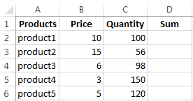
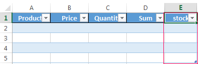
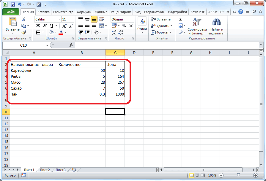
- Fill in the header manually by entering the column headings. Fill in the rows by entering your data. Apply the acquired knowledge in practice: expand the column boundaries, adjust the row height.
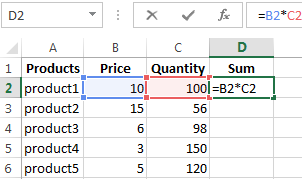
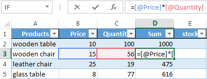
- To fill in the «Sum» column, place the cursor in its first cell. Enter «=». In such a way, we inform Excel: a formula will be here. Select the cell B2 (with the first price). Enter the multiplication symbol (*). Select the cell C2 (with the quantity). Press ENTER.
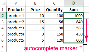
- When you hover the pointer over the cell containing the formula, a small cross will appear in its bottom right corner. It points out the autocomplete marker. Grab it with the left mouse button and drag it to the end of the column. The formula will be copied into every cell.
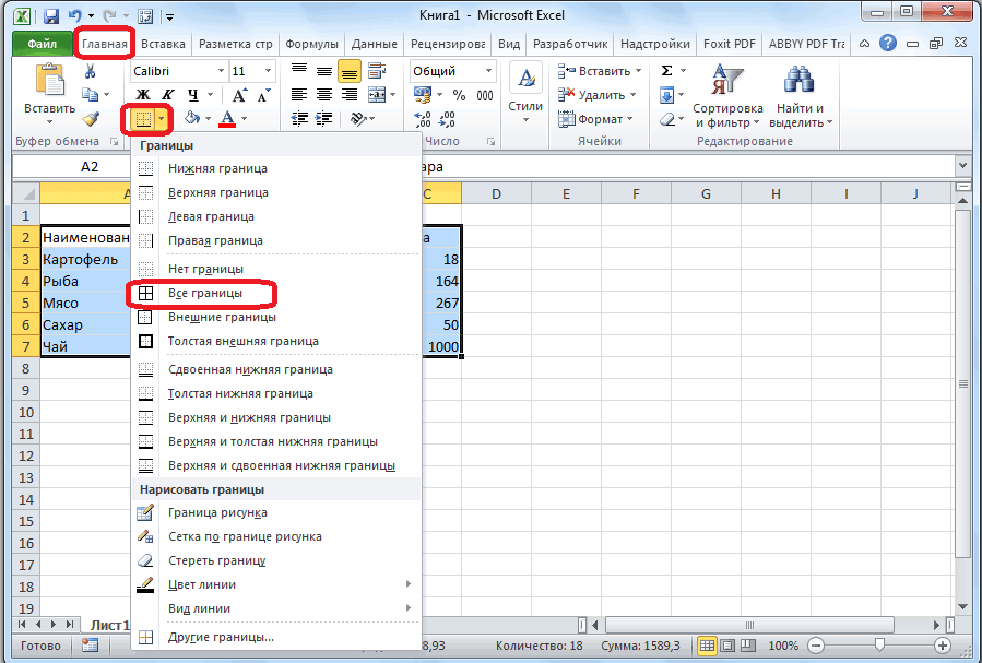
- Designate the boundaries of your table. Select the range containing your data. Click the button «HOME»-«Border» (on the main page in the «Font» menu). And click «All Borders».
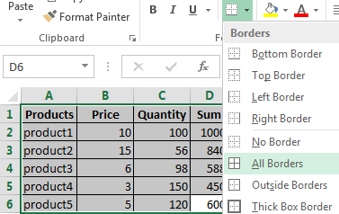
Now the column and row borders will be visible when you print the table.
The «Font» menu allows you to format the data in your Excel table the way you would do it in Word.
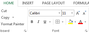
For example, change the font size and highlight the header in bold. You may also apply center alignment, word wrap, etc.
Creating a table in Excel: a step-by-step instruction
You already know the simplest way to create tables. However, Excel can offer a more convenient variant (in terms of the subsequent formatting and work with the data).
Let us construct a smart (dynamic) table:
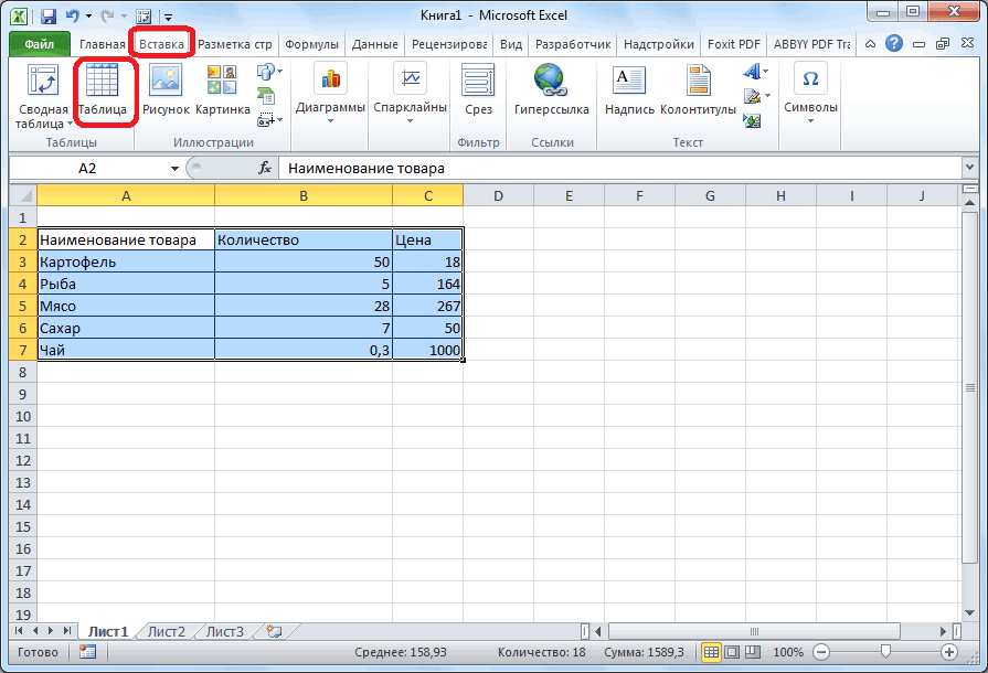
- Go to the «INSERT» tab – the «Table» tool (or press the hot-key combination CTRL+T).
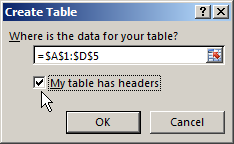
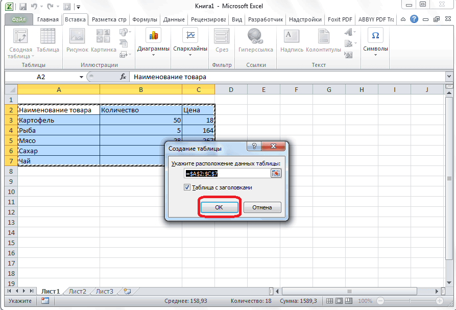
- This will open a dialog window, in which you need to enter the data range. Check the box for a table with headings. Click OK. It’s no big deal if you don’t enter the proper range on the first try. The smart table is flexible, dynamic.
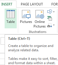
Important note. You can also take an alternative route: start with selecting the range of cells, then press the «Table» button.
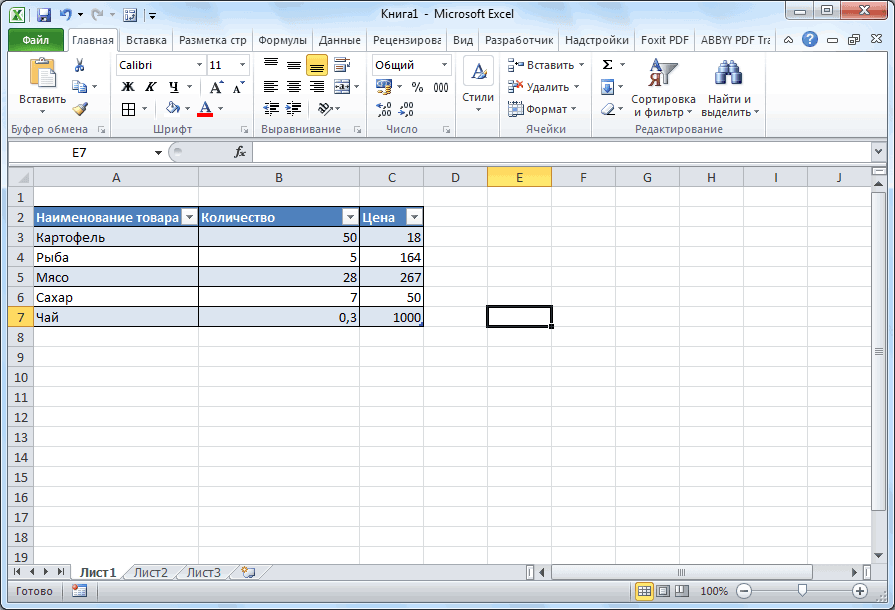
Now enter your data into the ready framework. If you need an additional column, place the cursor in the heading cell. Make the entry and press ENTER. The range will expand automatically.

If you need additional rows, grab the autocomplete marker in the bottom right corner and drag it downward.
How to work with a table in Excel
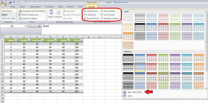
With the release of new versions of the program, working with tables in Excel has become more interesting and dynamic. After a smart table has been formed on the spreadsheet, the tool «TABLE TOOLS» — «DESIGN» becomes available.
Here you can name the table or resize it.
Various styles are available to you, as well as the opportunity to transform the table into a regular range or a consolidated sheet.
MS Excel dynamic electronic tables offer immense opportunities. Let us begin with the basic skills of data entry and autocompletion:
- Select a cell by clicking on it with the left mouse button. Enter the text/numeric value. Press ENTER. If you need to change the value, place the cursor in the cell again and enter the new data.
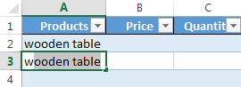
- When you enter a value repetitively, Excel will recognize it. You will only need to enter several symbols and press enter.
- In a smart table, to apply a formula to the entire column, enter it in the first cell. The program will copy the formula in other cells automatically.
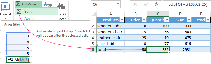
- To calculate the totals, select the column containing the values plus an empty cell for the future total and click the «Sum» button (the «Editing» tool group on the «HOME» tab, or press the hot-key combination ALT+»=»).
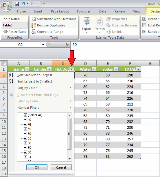
When you click on the little arrow to the right of every subheading in the header, you obtain access to the additional tools for working with the data in the table.
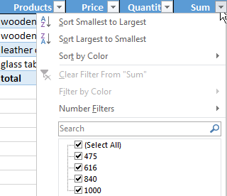
Sometimes the user has to work with huge tables, in which you need to scroll several thousand rows to see the totals. Deleting the rows is not an option (you will still need the data later). However, you can hide them. To this end, use number filters (depicted in the image above). Uncheck the values that need to be hidden.
What are Excel Tables?
Tables in Excel helps group related data into one or more rows and/or columns. Once a table is created, Excel assigns a unique name to the columns and the table itself. Such names are used as structured references, which make it easy to apply Excel formulas. Therefore, tables eliminate the need to create named ranges in Excel.
For example, the following image shows a usual data range on the left side and an Excel table on the right side. Notice the alternately colored excel rowsThe two different methods to add colour to alternative rows are adding alternative row colour using Excel table styles or highlighting alternative rows using the Excel conditional formatting option.read more and structured references (in cell J2) of the latter.
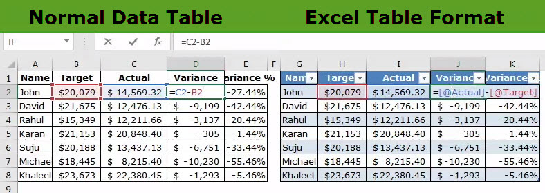
The purpose of creating tables is to make the data manageable, organized, and fit for analysis. Apart from structured references, tables offer several benefits like quick sorting and filtering, automatic expansion, easy formatting, readable formulas, and so on. Tables are extremely helpful when working with large databases.
Table of contents
- What are Excel Tables?
- How to Create Tables in Excel?
- How to Customize Tables in Excel?
- #1–Change the Name of the Table
- #2–Change the Color of the Table
- What are the Advantages of Creating Tables in Excel?
- #1–Creates Structured References Automatically
- #2–Is Dynamic in Nature
- #3–Makes it Easy to Work With PivotTables
- #4–Freezes Header Row Automatically
- #5–Helps add a Total Row Containing Functions
- #6–Eases Restoring to Usual Data Range Without Losing the Table Style
- #7–Helps add Slicers for Filtering Data
- #8–Assists in Creating Reports in Power BI
- How to Turn off Structured References in Excel?
- Frequently Asked Questions
- Recommended Articles
How to Create Tables in Excel?
You can download this Excel Tables Template here – Excel Tables Template
The steps to create a table in Excel are listed as follows:
- Ensure that the raw data does not contain any empty rows and/or columns. Further, each column should have a unique heading. If any two columns have the same headers, Excel automatically changes one of these headers once a table is created.
The raw data is shown in the following image.
Note: A column header should not contain any Excel formulas.

- Select any cell of the raw data and press the shortcut “Ctrl+T.” Both keys of the shortcut should be pressed together.
Note: Alternatively, after selecting a cell of the raw data, click “table” from the Insert tab of Excel. This option is in the “tables” group of the Excel ribbon.

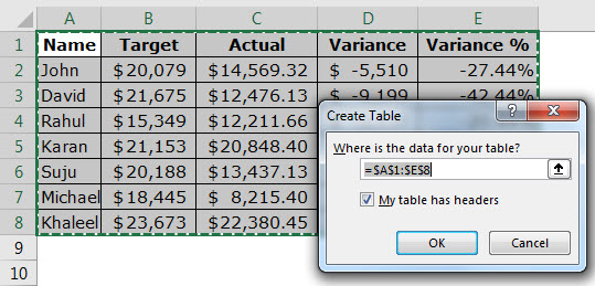
- The “create table” dialog box opens, as shown in the following image. Excel automatically selects the range for the table. Check whether this range is correct or not. If not, it can be edited.

- Select or deselect the checkbox of “my table has headers.” If selected, Excel will treat the content of the first row (row 1) as column headers.
In the preceding table, row 1 does contain column headers. So, we have selected the option “my table has headers.” Next, click “Ok.”

- An Excel table has been created. It is shown in the following image. Notice that the banded rows and filters (to the right of each column header) appear automatically.
Note: In Excel, banded rows are those in which color or shading is applied alternately.


How to Customize Tables in Excel?
A table can be customized by changing its name and/or the default color (or table style). Let us learn how this is done.
#1–Change the Name of the Table
When a table is created, Excel assigns a default name like “table1,” “table2,” etc., depending on whether it is the first or the second table of the current workbook.
Working with such default names may become confusing, especially when there are lots of tables. So, the solution is to assign unique names to each table.
The steps for changing the name of the Excel table are listed as follows:
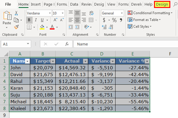
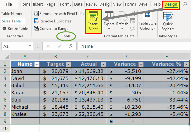
Step 1: Select the entire table. Once selected, the Design tab appears on the Excel ribbonRibbons in Excel 2016 are designed to help you easily locate the command you want to use. Ribbons are organized into logical groups called Tabs, each of which has its own set of functions.read more. This tab is shown within a red box in the following image.
Note: In place of the entire table, even if a single cell is selected, the Design tab will become visible.
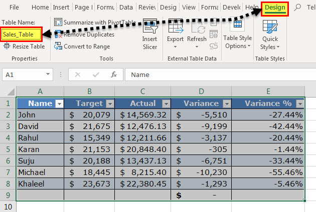
Step 2: In the Design tab, perform the following tasks:
- Click inside the box under “table name.” This box is displayed in the “properties” group at the leftmost side of the ribbon.
- Enter the desired name in this box.
- Press the “Enter” key.
Our table has been named “Sales_Table.” This is shown in the following image.
Rules Governing the Table Names
While naming a table, the following points should be considered:
- The name should always begin with a letter, a backslash () or an underscore (_).
- The name cannot be the single letter “r” (or “R”) or “c” (or “C”).
- The name should not consist of any spaces. Instead, one can use an underscore (_) or a period (.) to separate the words.
- The name can contain numbers, but cell references should be avoided.
- The name can contain a maximum of 255 characters.
- The name of the table should be unique. In case of a duplicate name, a message will be displayed saying that a unique name should be chosen.
Note: A name is said to be duplicate if two tables within the same workbook have the same names. Further, Excel does not distinguish between the uppercase and lowercase letters in the name of a table. So, the names “abc” or “ABC” are considered the same by Excel.
#2–Change the Color of the Table
When a table is created, Excel assigns it a default color. To change the color of the table, its style needs to be changed. Excel displays a list of different table styles from which one can choose the desired option.
The steps to change the color (or style) of a table are listed as follows:
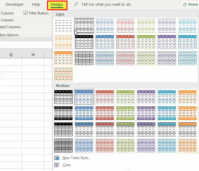
Step 1: Select either a cell of the table or the entire table. We have selected the latter. The Design tab becomes visible, as shown in the following image.

Step 2: Choose the desired color (or style) from the “table styles” group of the Design tab. To expand the list of table styles, click the “more” button displayed at the bottom right side. One can also click “new table style” to view more styles.
The following image shows the expanded list of table styles. Once the desired style is chosen, it will be applied to the entire table.
Note: The default table style of the workbook can be changed by the user. For making this change, perform the listed steps:
- Select the desired table style from the list of table styles.
- Right-click the selected table style and choose “set as default” from the context menu.
What are the Advantages of Creating Tables in Excel?
Let us discuss eight advantages of creating tables in Excel.
#1–Creates Structured References Automatically
An Excel table uses structured referencesIn Excel, structured references define data sets in columns by giving names instead of cell address. You may use the column name instead of the cell address in the formula; this makes work easier.read more for referencing one or more cells. This is in contrast with the direct cell addresses used in a normal data range. A structured reference is a combination of table and column names that are used in Excel formulasThe term «basic excel formula» refers to the general functions used in Microsoft Excel to do simple calculations such as addition, average, and comparison. SUM, COUNT, COUNTA, COUNTBLANK, AVERAGE, MIN Excel, MAX Excel, LEN Excel, TRIM Excel, IF Excel are the top ten excel formulas and functions.read more.
The major benefits of using structured references are listed as follows:
- They automatically update when new entries are added or deleted from the table.
- They are automatically created when one or more cells of the table are selected.
- They can be used both within and outside the table, thus making it easy to locate tables in a workbook.
- They are used to autofill the calculated columns. A calculated column is an additional column added to the existing Excel table. It uses a single formula that expands on its own in the remaining part of the column. This implies that when a formula is entered in one cell of a calculated column, it need not be dragged to the remaining cells of the column. Rather, the formula is automatically entered in all cells (called autofill), unlike a usual data range which requires one to drag the fill handleThe fill handle in Excel allows you to avoid copying and pasting each value into cells and instead use patterns to fill out the information. This tiny cross is a versatile tool in the Excel suite that can be used for data entry, data transformation, and many other applications.read more.
Example of point “d”: The range A2:B7 is an Excel table containing random numbers. To create column C as a calculated column, enter the SUM formula in cell C3, which adds the numbers of cells A3 and B3. Use structured references in this formula. Once the formula is entered, press the “Enter” key. The outcomes are stated as follows:
- The table (A2:B7) automatically expands to include column C.
- The range C4:C7 is automatically filled with the totals of each row of the table.
The preceding results will be obtained with both structured and regular references. This is because autofilling is a feature of Excel tables. However, with structured references, it is easy to read and understand the formula.
Note that if the user makes a change to the formula of the calculated column, the change is automatically replicated in the entire column.
Example of structured references: In the following image, structured references have been used in the SUMIF formula. The “Calls_Table” is the name of the Excel table. “Day” and “duration” are the names of columns A and E respectively. The cell G2 is a direct cell referenceCell reference in excel is referring the other cells to a cell to use its values or properties. For instance, if we have data in cell A2 and want to use that in cell A1, use =A2 in cell A1, and this will copy the A2 value in A1.read more.
Note: In the following image, the black line pointing to cell G2 has been incorrectly placed. It should have pointed to “day,” which is the name of column A. So, please ignore the misplacement.

#2–Is Dynamic in Nature
Any new insertions to the cells below or to the right of the table are automatically included in the Excel table. This implies that the table expands to include such insertions. Likewise, the table contracts when one or more rows and/or columns are deleted from it. Due to automatic expansion and contraction, an Excel table is often considered a dynamic tableDynamic tables in Excel are ones in which the table automatically adjusts its size when a new value is inserted. It can be done in one of two ways: by using the offset function or by creating a data table from the table section.read more.
Expansion implies that the style, formatting, and formulas of the table are automatically applied to the new entries as well. This eliminates the need to format and edit the formulas of individual cells. By default, the formatting stays uniform throughout an Excel table.
Note that the formulas of the table are adjustable as they take into account structured references. In contrast, the formulas of a normal data range do not adjust with insertions or deletions of entries.
Note: To undo table expansion, press the keys “Ctrl+Z” together.
#3–Makes it Easy to Work With PivotTables
It is advised to create a PivotTableA Pivot Table is an Excel tool that allows you to extract data in a preferred format (dashboard/reports) from large data sets contained within a worksheet. It can summarize, sort, group, and reorganize data, as well as execute other complex calculations on it.read more from an Excel table. The major reasons the source data should be an Excel table are listed as follows:
- A PivotTable automatically updates with any changes in the source table. Since Excel tables are dynamic, the data range of the PivotTable also becomes dynamic.
- A single cell of the source table can be selected prior to inserting a PivotTable. In contrast, when the source data is a usual data range, the entire range (or dataset) needs to be selected prior to inserting a PivotTable.
For instance, in the following image, a single cell of the source table has been selected before clicking the “PivotTable” option from the Excel Insert tabIn excel “INSERT” tab plays an important role in analyzing the data. Like all the other tabs in the ribbon INSERT tab offers its own features and tools. Under Insert Tab we have several other groups including tables, illustration, add-ins, charts, Power map, sparklines, filters, etc.read more. Notice that in “table/range,” the name of the source table is reflected.

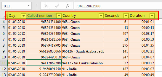
When one scrolls downwards in a worksheet, the table headers are visible at all times. This is because these headers are automatically fixed or frozen at their respective places.
Fixed headers prevent the user from going back to the top row (row 1) again and again. Such frozen headers can be seen within a red rectangle in the following image.
Notice that the user has scrolled downwards such that rows 4 to 13 are visible along with the header row.
Note: To see the frozen header row, ensure that a cell of the table is selected before scrolling.
#5–Helps add a Total Row Containing Functions
An Excel table shows various functions in the total row. For displaying this row, perform the following steps:
- Select any cell of the Excel table. The Design tab appears on the Excel ribbon.
- From the Design tab, select the checkbox of “total row” displayed in the “table style options” group.
The total row is added immediately below the Excel table. Select any cell of this row to see a drop-down arrow on the right side. When this arrow is clicked, a list containing functions appears, as shown in the following image.
Once a function is selected from the list, the respective formula is automatically entered and the output is shown in a cell of the total row.
Notice that row 9 of the following image is the total row. Further, if a function is selected in cell D9, the corresponding output will also be displayed in this cell. The formula will be visible in the formula bar of the worksheet.

#6–Eases Restoring to Usual Data Range Without Losing the Table Style
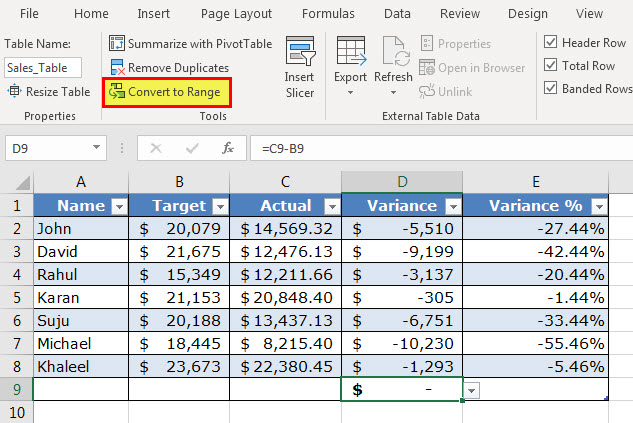
An Excel table can be quickly converted to a usual data range. This serves as a benefit when the user requires only the table style and not the functionality of the table. For such conversion, follow either of the listed steps:
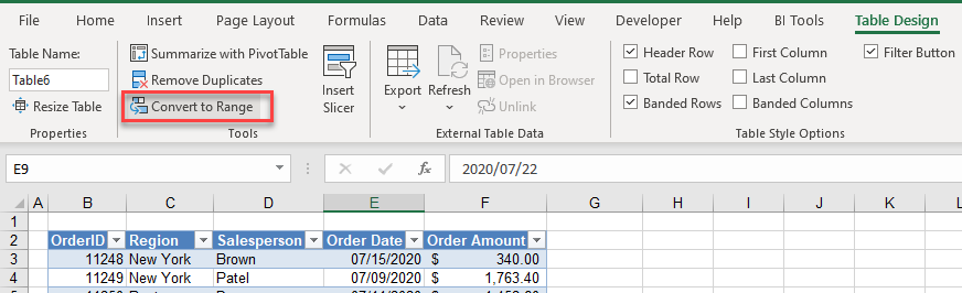
- Select any cell of the table. From the Design tab, click “convert to range” in the tools group.
- Select any cell of the table and right-click it. From the context menu, choose “table” followed by “convert to range.”
The “convert to range” feature of the first pointer is shown in the following image. Once an Excel table is converted to a usual data range, the existing structured references are replaced with the regular cell references. However, the data and formatting of the table are retained in the usual data range.
Note: The “convert to range” feature can be used only when the data to be converted is in the form of an Excel table.
#7–Helps add Slicers for Filtering Data
A slicer helps filter the data of an Excel table. It displays buttons that can be selected or deselected to indicate whether an item is included or excluded from the filter.
Slicers are available in Excel 2013 and the newer Excel versions. The steps to add a slicer to a table are listed as follows:
- Select either a cell within the table or the entire table.
- From the Design tab, select “insert slicer” from the “tools” group.
- The “insert slicer” dialog box opens. Next, select the checkboxes of the columns for which the slicer needs to be created.
- Click “Ok.”
One can have a slicer for each column of the Excel table. Once slicers appear in the worksheet, they can be moved, resized, and formatted according to the requirement.
With a slicer, one can filter and view only particular items (or entries) of the table. To view multiple items of a column, press and hold the “Ctrl” key while selecting the items in the respective slicer.
The following image shows the “insert slicer” option of the Design tab.
Note 1: A slicer can also be added from the “filters” group of the Insert tab of Excel. Click “slicer” in this group and thereafter follow the steps “c” and “d” listed above.
Note 2: A slicer can be used only if the data is in the form of an Excel table.
#8–Assists in Creating Reports in Power BI
Excel tables serve as a source from which data is entered in the Power BI tool. Power BI is a business intelligence tool that helps convert unrelated sources of data into meaningful reports and dashboards. The process of creating reports works as follows:
- Create and upload Excel tables to Power BI.
- Create a report in Power BI by adding visualizations.
- Share the report with other Power BI users or office colleagues.
Excel tables are a preferred data source in Power BI due to the following reasons:
- They allow quick access to the tabular format of the dataset.
- They help ease comparisons within a dataset.
- They can be easily edited and organized prior to being uploaded in Power BI.
How to Turn off Structured References in Excel?
The steps to turn off structured references in Excel are listed as follows:
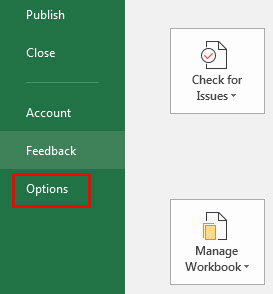
Step 1: Click the File tab of Excel. It is displayed within a red box in the following image.

Step 2: Select “options” shown in the following image.
Step 3: The “Excel options” dialog box opens. Click “formulas” appearing on the left side of the window. Deselect the checkbox of “use table names in formulas.” This is shown in the following image.
Next, click “Ok.” The structured references will be turned off in Excel.
Note: By changing this setting, the structured references used in the existing formulas of the Excel table are not removed. However, the new formulas applied to the table will contain regular cell references instead of structured references. If regular cell references are required in existing formulas too, they will have to be edited manually.
Further, whether the structured references are turned on or off, the changed setting will be applied to all workbooks that the user is working on.

Frequently Asked Questions
1. What are Excel tables and how are they created?
An Excel table displays the data in a tabulated format. Every column should have unique headers (or names) according to the kind of data they contain. Such headers are placed in the top row of the table. The table may or may not be named by the user.
If the columns and table are not named by the user, Excel assigns default names to both of them. These names are used as structured references in all formulas applied within or outside the table (that contain a table reference).
To create a table in Excel, select any cell of the dataset and press the keys “Ctrl+T” or “Ctrl+L.”
2. How to join two tables in Excel?
Two tables that have a common column can be joined with the help of the VLOOKUP function of Excel. The formula is stated as follows:
“=VLOOKUP(lookup_value,entire_lookup_table,return_column,FALSE)”
For instance, the first table is named “table1” and the second table is named “table2.” To pull the data of a single column of “table2” in “table1,” enter the following formula:
“=VLOOKUP($A2,table2,3,FALSE)”
This formula looks up the value of cell A2 in “table2.” It returns an exact match from the third column of “table2.”
One can use either regular or structured references in the given formula. By selecting the cell of the “lookup_value” and the range of the “entire_lookup_table,” Excel will automatically enter structured references in the VLOOKUP formula.
Note 1: Enter the given formula in the first cell to the immediate right of the first table. Once entered, press the “Enter” key. The Excel table expands to include the new column. Consequently, the outputs of the entire column are displayed in the first table.
Note 2: For the given formula to work, the column containing the “lookup_value” should be common to both tables. Moreover, the lookup column (containing the “lookup_value”) should be the leftmost column of the second table. The return column (containing the value to be returned) of the second table should be to the right of the lookup column.
3. When should Excel tables be used and how to locate them in a workbook?
Excel tables should be used in the following situations:
• To arrange data in a tabular format
• To facilitate comparisons of data values
• To improve the readability of the dataset
• To ease data analysis and eventually assist in decision-making
To locate tables in a workbook, click the downward arrow appearing on the right side of the name box. It shows the names of all the tables of the workbook. Clicking on any of these names will select that particular table.
Recommended Articles
This has been a guide to tables in Excel. Here, we explain how to create/insert/customize Excel tables along with examples and advantages. You may also look at these useful functions of Excel–
- Delete Pivot Table ExcelTo delete a pivot table in Excel, you must first select it. Then go to the Analyze menu tab under the Design and Analyze menu tabs and select actions. Then, from the Select option’s drop-down option, select Entire Pivot Table to delete it.read more
- Refresh Pivot Table in ExcelTo refresh pivot tables, you may use the following methods — refresh pivot table by changing data source, refresh pivot table using right click option, auto-refresh pivot table using VBA Code, refresh pivot table when you open the workbook.read more
- Data Table in Excel
- Excel Merge Tables We can use a number of different methods to merge tables in Excel, including the VLOOKUP function, the INDEX function, and the MATCH function.read more
This tutorial demonstrates how to create a table in Excel.
Create an Excel Table
You can either create an Excel table using existing data, or you can create a blank table and fill it with data afterwards.
- To create a table using existing data, ensure that your data is laid out in a way that is compatible with creating a table, e.g., each column should have a header row that describes the contents of that column and no blank rows or columns should exist in the middle or the data.
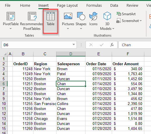
- Then, in the Ribbon, go to Insert > Table.
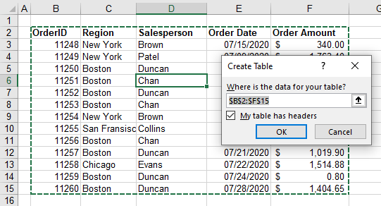
- Excel selects the entire range of data. Leave My table has headers ticked, and then click OK.
- This automatically creates a table as far down as the next blank row and as far across as the next blank column.
Alternate Shading in a Table
When a table is automatically created, the table is formatted according to the default table style that exists in Excel. This means that the top row is formatted with a blue background and white writing, while the rows below are formatted alternatively with a blue or white background.
- To change the table’s appearance, click somewhere within the table and in the Ribbon, go to Table Design > Table Styles. Choose a style.
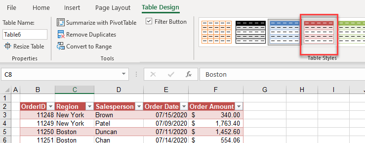
- The format changes according to the style you choose. There are many built-in styles available. To access a few more styles, click the “more” button as shown below.
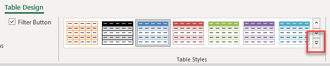
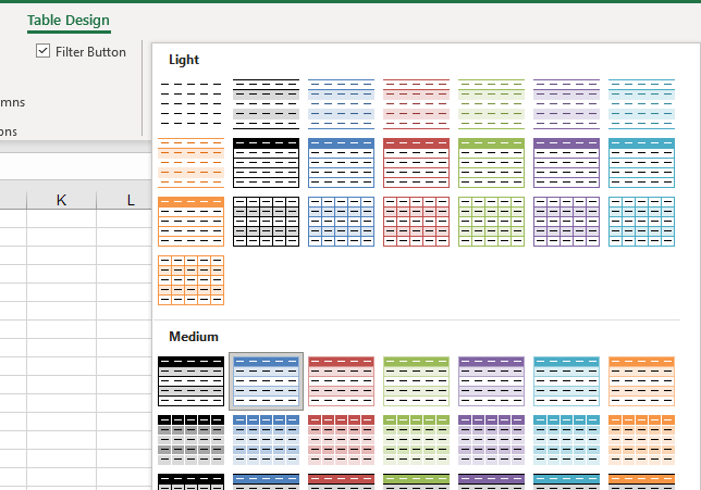
- The list of styles is expanded to show a variety of different table styles. Choose one.
Convert Table Back to a Range
If you have formatted your data as a table, and then wish to remove the filter options and convert your table back to a range, you can use the Table Design tab to do this.
- Click in your table, and then in the Ribbon, go to Table Design > Tools > Convert to Range.
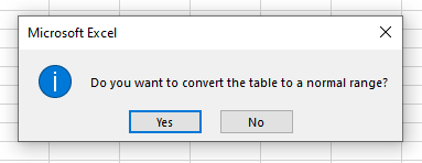
- Click OK to convert your table to a range.
While the formatting is preserved, the filters are removed from the column headers indicating that the data is now a normal range and no longer a table.
Link Tables: Relationships
If you have data in two different ranges in Excel, but the data is linked together by a common column name, you can create a relationship between these two sets of data as long as both sets of data are tables in Excel.
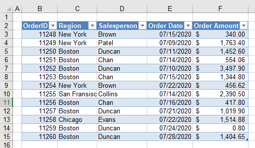
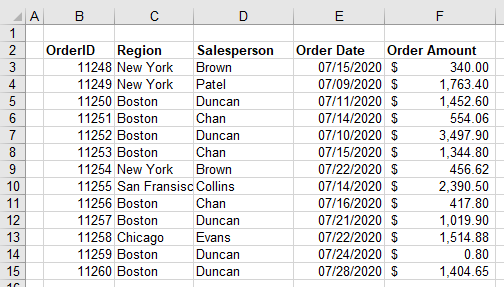
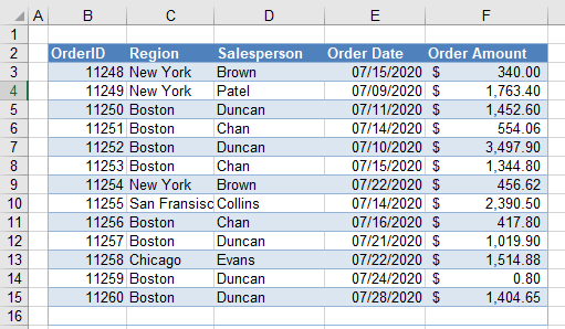
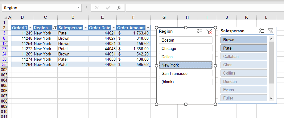
Consider the following two tables in Excel.
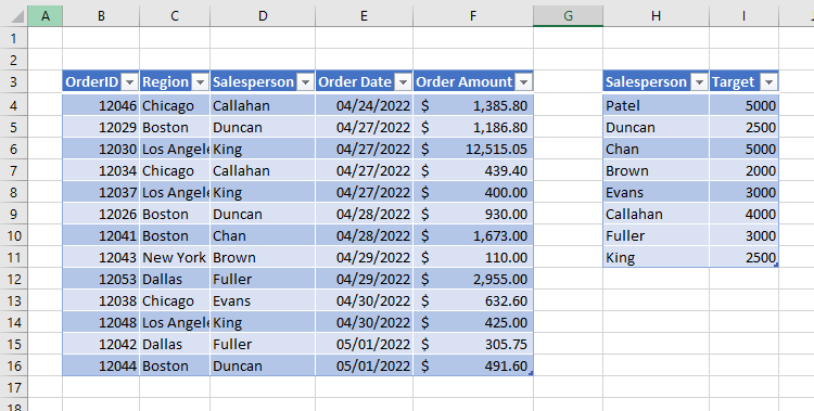
One table contains the salesperson‘s name and their Sales Target, while the other table contains their order amounts. In one table, the salesperson appears only once while in the other table the salesperson can appear multiple times.
Note: the data does not have to be on one sheet and may be much larger than the example above.
For example, to create a pivot table that contains information from both tables, you can link these tables together by creating a relationship between them.
Note: Try using some shortcuts when you’re working with pivot tables.
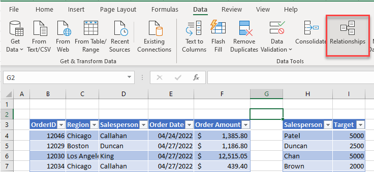
- In the Ribbon, go to Data > Data Tools > Relationships.
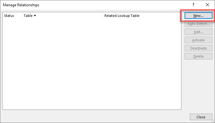
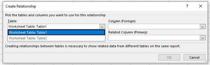
- In the Relationships window, click New.
- In the Table drop down, choose the first table and in the drop down below, choose the second table.
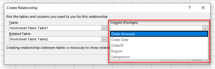
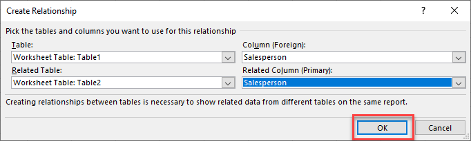
- In the Column table, first choose the Foreign column (in this case, Salesperson as it can appear multiple times); and then in the Related Column, choose the Salesperson field from the second table. This is the Primary column where the salesperson only appears once in that table.
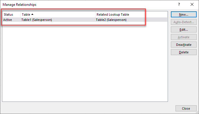
- Click OK to create the relationship.
- Click Close to return to Excel.
Benefits of Using a Table
Add Totals Automatically
Adding a total row to a table is incredibly easy.
Click in your table, and then, in the Ribbon, go to Table Design > Table Style Options > Total Row
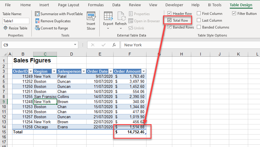
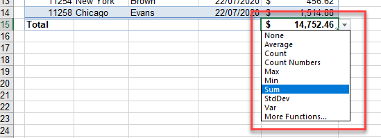
The default function use for the Total Row is the sum function. You can, however, amend this function if you want to use a different function.
Notice that the Header Row, Banded Rows, and Filter Button are also ticked in this group of options.
- If you switch off the Header Row, then the Filter Button option is no longer available.
- If you switch off the filter option, you can’t use the filter option in your table.
- you switch off the Banded Rows option, the rows are no longer alternatively shaded.
Automatically Add Rows With Tab Key
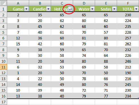
One of the benefits of using at table is that a table will automatically expand if you enter more data into the table. Notice that in the bottom row of the table, a small, backward-L-shaped handle exists.
![]()
If you then click in this cell and press the TAB key, a new row in the table is created, and your cursor is moved to the first cell in the new row. The table has therefore automatically expanded to include this row.
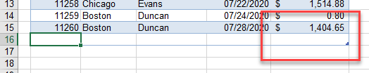
This is useful since some of the benefits of using a table are the sorting and filtering options that are built into the table. If you then wanted to filter on the Salesperson, for example, the new record is automatically included in that filter. Similarly, if you sort the data, the new row(s) are included in the sort.
Consistent Formulas
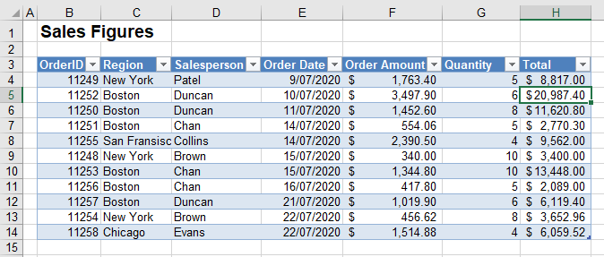
If you add two more columns to the table, these would automatically be included in the table, as the new rows were above.
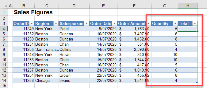
Then, add a formula to work out the total by multiplying the Order Amount by the Quantity. The formula is created using the field names (column headers).
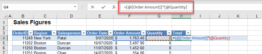
When you press ENTER, the formula is copied down to all the other rows in the table.
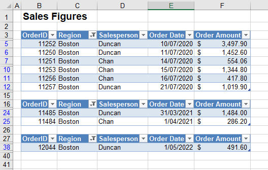
Multiple Filters on One Sheet
In the example below, a table has been created for each year of orders, and then, each table has been filtered by region to show the orders for a single region in each individual year.
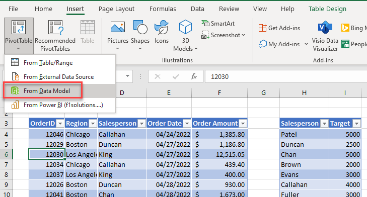
Combine Tables Into One Pivot Table
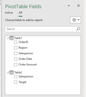
If you have created a relationship between two tables, you can create a pivot table using fields from both tables.
- In the Ribbon, go to Insert > Pivot Table > From Data Model.
- Select New Worksheet, and then click OK.
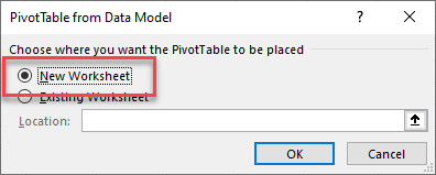
- You now have the field available from both your tables to use in your pivot table where the linked fields (Salesperson) will show up identical data.
Able to Use Slicers
When you data is formatted as a table, you are able to use slicers to filter your data.
- Click in your table and then, in the Ribbon, select Table Design > Tools > Insert Slicer.
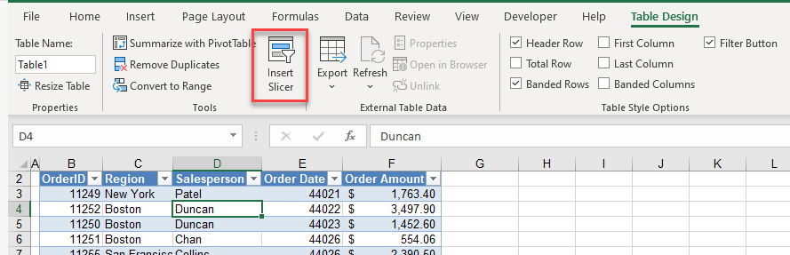
- Select the field or fields of the slicer you wish to insert, and then click OK.
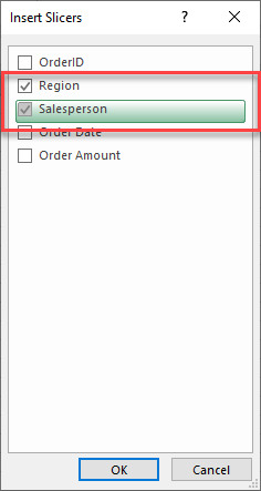
- You can then filter your data by selecting an individual value in the slicer, or you can hold down the CTRL key (for nonconsecutive values) or the SHIFT key (for consecutive values) to filter on multiple values.
PowerPivot and Power Query
Any data used in a Power Pivot or Power Query must be in a table format. So for users of Power Query, formatting as an Excel table is a necessity, not just a benefit.
More on Tables
| Tables | |
|---|---|
| Add a Column and Extend a Table | |
| Add a Total or Subtotal Row to a Table | |
| Compare Two Tables | |
| Convert a Table to a Normal Range | |
| Display Data With Banded Rows | |
| Remove a Table or Table Formatting | |
| Rename a Table | |
| Rotate Data Tables | |
| Conditional Formatting | yes |
| Highlight Every Other Line In Excel | |
| Copy & Paste | yes |
| Copy Every Other Row | |
| Database | yes |
| Create a Searchable Database | |
| Filters | yes |
| Filter Rows | |
| Find & Select | yes |
| Select Every Other Row | |
| Format Cells | yes |
| Alternate Row Color | |
| Insert & Delete | yes |
| Delete Every Other Row |
In this post, we’re going to learn everything there is to know about Excel Tables!
Yes, I mean everything and there’s a lot.
This post will tell you about all the awesome features Excel Tables have and why you should start using them.
What is an Excel Table?
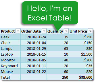
Excel Tables are containers for your data.
Imagine a house without any closets or cupboards to store your things, it would be chaos! Excel tables are like closets and cupboards for your data, they help to contain and organize data in your spreadsheets.
In your house, you might put all your plates into one kitchen cupboard. Similarly, you might put all your customer data into one Excel table.
Tables tell excel that all the data is related. Without a table, the only thing relating the data is proximity to each other.
Ok, so what’s so great about Excel Tables other than being a container to organize data? A lot actually. This post will tell you about all the awesome features tables have and should convince you to start using them.
Video Tutorial
The Parts of a Table
Throughout this post, I’ll be referring to various parts of a table, so it’s probably a good idea that we’re both talking about the same thing.
This is the Column Header Row. It is the first row in a table and contains the column headings that identify each column of data. Column headings must be unique in the table, they cannot be blank and they cannot contain formulas.
This is the Body of the table. The body is where all the data and formulas live.
This is a Row in the table. The body of a table can contain one or more rows and if you try to delete all the rows in a table a single blank row will remain.
This is a Column in the table. A table must contain at least one column.
This is the Total Row of the table. By default, tables don’t include a total row but this feature can be enabled if desired. If it’s enabled, it will be the last row of the table. This row can contain text, formula or remain blank. Each cell in the total row will have a drop down menu that allows selection of various summary formula.
Create a Table from the Ribbon
Creating an Excel Table is really easy. Select any cell inside your data and Excel will guess the range of your data when creating the table. You’ll be able to confirm this range later on. Instead of letting Excel guess the range you can also select the entire range of data in this step.
With the active cell inside your data range, go to the Insert tab in the ribbon and press the Table button found in the Tables section.
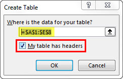
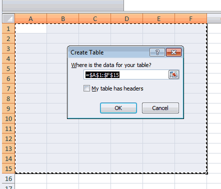
The Create Table dialog box will pop up. Excel guesses the range and you can adjust this range if needed using the range selector icon on the right hand side of the Where is the data for your table? input field. You can also adjust this range by manually typing over the range in the input field.
Checking the My table has headers box will tell Excel the first row of data contains the column headers in your table. If this is unchecked Excel will create generic column headers for the table labelled Column 1, Column 2 etc…
Press the Ok button when you’re satisfied with the data range and table headers check box.
Congratulations! You now have an Excel table and your data should look something like the above depending on the default style of your tables.
Contextual Table Tools Design Tab
Whenever you select a cell inside a table, you will notice a new tab appear in the ribbon labelled Table Tools Design. This is a contextual tab and only appears when a table is selected. When the active cell moves outside the table, the tab will disappear again.
This is where all the commands and options related to tables will live. This is where you’ll be able to name your table, find table related tools, enable or disable table elements and change your table’s style.
Create a Table with a Keyboard Shortcut
You can also create a table using a keyboard shortcut. The process is the same as described above but instead of using the Table button in the ribbon you can press Ctrl + T on your keyboard. It’s easy to remember since T is for Table!
There is actually another keyboard shortcut that you can use to create tables, Ctrl + L will also do the same thing. This is a legacy from when tables were called lists (L is for List).
Name a Table
Anytime you create a new table Excel will give it an initial generic name starting with Table1 and increasing sequentially. You should always rename your table with a descriptive and short name.
Not all names are allowed. There are a few rules for a table name.
- Each table must have a unique name within a workbook.
- You can only use letters, numbers and the underscore character in a table name. No spaces or other special characters are allowed.
- A table name must begin with either a letter or an underscore, it can not begin with a number.
- A table name can have a maximum of 255 characters.
Select any cell inside your table and the contextual Table Tools Design tab will appear in the ribbon. Inside this tab you can find the Table Name under the Properties section. Type over the generic name with your new name and press the Enter button when finished to confirm the new name.
Rename a Table
Renaming a table you’ve already named is the same process as naming a table for the first time. If you think about it, when you first name a table you’re actually renaming it from the generic name of Table1 to a new name.
So go back to the Table Tools Design tab and type your new name over the old one in the Table Name and press Enter. Easy, and the name is changed.
Changing your table name this way requires navigating to your table and selecting a cell within it, so it can be tedious if you need to rename a lot of tables across different sheets in your workbook. Instead, you can change any of your table names without going to each table using the Name Manager.
Go to the Formula tab and press the Name Manager button in the Defined Names section. You’ll be able to see all your named objects here. The table objects will have a small table icon to the left of the name. You can filter to show only the table objects using the Filter button in the upper right hand corner and selecting Table Names from the options.
You can then edit any name by selecting the item and pressing the Edit button. You’ll be able to change the name and add some comments to describe the data in your table.
Navigate Tables with the Name Box
You can easily navigate to any table in your workbook using the name box the the left of the formula bar. Click on the small arrow on the right side of the name box and you will see all table names in the workbook listed. Click on any of the tables listed and you will be taken to that table.
Convert a Table Back to a Normal Range
Ok, you changed your mind and don’t want your data inside a table anymore. How do you convert it back into a regular range?
If changing it to a table was the last thing you did, Ctrl + Z to undo your last action is probably the quickest way.
If it wasn’t the last thing you did, then you’re going to need to use the Convert to Range command found in the Table Tools Design tab under the Tools section.
You’ll be prompted to confirm that you really want to convert the table to a normal range. Noooooo, don’t do it, tables are awesome!
If you click on yes, then all the awesome benefits from tables will be gone except for the formatting design. You’ll need to manually clear this from the range if you want to get rid it. You can do this by going to the Home tab then pressing the Clear button found in the Editing section, then selecting Clear Formats.
This can also be done from the right click menu. Right click anywhere in the table and select Table from the menu and then Convert to Range.
Select the Entire Column
If your data is not inside a table then selecting an entire column of the data can be difficult. The usual way would be to select the first cell in the column and then hold Ctrl + Shift then press the Down arrow key. If the column has blank cells, then you might need to press the Down arrow key a few times until you reach the end of the data.
The other option is to select the first cell and then use the scroll bar to scroll to the end of your data then hold the Shift key while you select the last column.
Both options can be tedious if you have a lot of data or there are a lot of blanks cells in the data.
With a table, you can easily select the entire column regardless of blank cells. Hover the mouse cursor over the column heading until it turns into a small arrow pointing down then left click and the entire column will be selected. Left click a second time to include the column heading and any total row in the selection.
Another way to quickly select the entire column is to place the active cell cursor on any cell in the column and press Ctrl + Space. This will select the entire column excluding the column header and total row. Press Ctrl + Space again to include the column headers and total row.
Select the Entire Row
Selecting the entire row is just as easy. Hover the mouse cursor over the left side of the row until it turns into a small arrow pointing left then left click and the entire row will be selected. This works on both the column heading row and total row.
Another way to quickly select the entire row is to place the active cell cursor on any cell in the row and press Shift + Space.
Select the Entire Table
It’s also possible to select the entire table and there are a couple different ways to do this.
You can place the active cell cursor inside the table and press Ctrl + A. This will select the entire body of the table excluding the column headers and total row. Press Ctrl + A again to include the column headers and total row.
Hover the mouse over the top left hand corner of the table until the cursor turns into a small black diagonal right and downward pointing arrow. Left click once to select only the body. Left click a second time to include the header row and total row.
You can also select the table with the mouse. Place the active cell inside the table and then hover the mouse cursor over any edge of the table until it turns into a four way directional arrow then left click. This will also select the column headers and total row.
Select Parts of the Table from the Right Click Menu
You can also select rows, columns or the entire table using the right click menu. Right click anywhere on the row or column you want to select then choose Select and pick from the three options available.
Add a Total Row
You can add a total row which allows you to display summary calculations in the last row of your table.
Adding summary calculations at the bottom of your data can be dangerous as they might end up getting included by accident in a pivot table using the data. This is another advantage of tables, as the total row won’t be included in any pivot tables created with the table.
To enable the total row, go to the Table Tools Design tab and check the Total Row box found in the Table Style Options section.
You can temporarily disable the total row without losing the formulas you added to it. Excel will remember the formulas you had and they will appear when you enable it again.
Each cell in the total row has a drop down menu that allows you to pick various aggregating functions to summarize the column of data above.
You can also enter your own formulas. I’ve entered a SUMPRODUCT formula in the Unit Price total to sum the Quantity x Unit Price to calculate a total sale amount. Formulas don’t have to return a number, they can also be text results.
Constant numerical or text values are also allowed anywhere in the total row. In fact the leftmost column will usually contain the text Total by default.
Add a Total Row with a Right Click
You can also add the total row with a right click. Right click anywhere on the table and the choose Table and Total Row from the menu.
Add a Total Row with a Keyboard Shortcut
Another way to quickly add the total row is to place the active cell cursor inside your table and use the Ctrl + Shift + T keyboard shortcut.
Disable the Column Header Row
The column header row is enabled by default, but you can disable it. This doesn’t delete the column headers, it’s essentially like hiding them as you will still reference columns based on the column header name.
Go to the Table Tools Design tab and uncheck the Total Row box found in the Table Style Options section.
Add Bold Format to the First or Last Columns
You can enable a bold formatting on either your first or last column to highlight it and draw attention to them over other columns.
Go to the Table Tools Design tab and check either of the First Column or Last Column boxes (or both) found in the Table Style Options section.
Add Banded Rows or Columns
Banded rows are already enabled by default, but you can turn them off if you want. Banded columns are disabled by default, so you need to enable them if you want them.
To enable or disable either, go to the Table Tools Design tab and check or uncheck the Banded Rows or Banded Columns boxes found in the Table Style Options section.
I generally find banded rows are the most useful and if you enable banded columns at the same time, the table starts to look a little messy. I recommend one or the other and not both at the same time.
- Table with no banded rows or columns.
- Table with banded rows only.
- Table with banded columns only.
- Table with both banded rows and columns.
Table Filters
By default, the table filters option is enabled. You can disable them from the Table Tools Design tab by unchecking the Filter Button box found in the Table Style Options section.
You can also toggle the filters on or off from the active table by using the regular filter keyboard shortcut of Ctrl + Shift + L.
If you left click on any of the filters, it will bring up the familiar filter menu where you can sort your table and apply various filters depending on the type of data in the column.
The great thing about table filters is you can have them on multiple tables in the same sheet simultaneously. You will need to be careful though as filtered items in one table will affect the other tables if they share common rows. You can only have one set of filters at a time in a sheet of data without tables.
Total Row with Filters Applied
When you select a summary function from the drop down menu in the total row, Excel will create the corresponding SUBTOTAL formula. This SUBTOTAL formula ignores hidden and filtered items. So when you filter your table these summaries will update accordingly to exclude the filtered values.
Note that the SUMPRODUCT formula in the Unit Price column still includes all the filtered values while the SUBTOTAL sum formula in the Quantity column does not.
Column Headers Remain Visible When Scrolling
If you scroll down while the active cell is in a table, its column headers will remain visible along with the filter buttons. The table’s column headings will get promoted into the sheet’s column headings where we would normally see the alphabetic column name.
This is extremely handy when dealing with long tables as you won’t need to scroll back up to the top to see the column name or use the filters.
Automatically Include New Rows and Columns
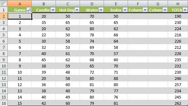
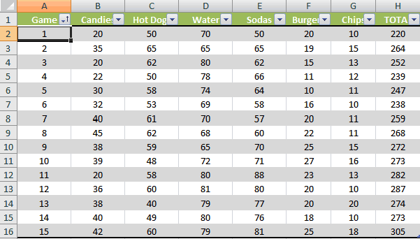
If you type or copy and paste new data into the cells directly below a table, they will automatically be absorbed into the table.
The same thing happens when you type or copy and paste into the cells directly to the right of a table.
Automatically Fill Formulas Down the Entire Column
When you enter a formula inside a table it will automatically fill the formula down the entire column.
Even when a formula has already been entered and you add new data to the row directly below the table any existing formulas will automatically fill.
Editing an existing formula in any of the cells will also update the formula in the entire column. You’ll never forget to copy and paste down a formula again!
Turn Off the Auto Include and Auto Fill Settings
You can turn off the feature that automatically adds new rows or columns and fills down formulas.
Go to the File tab and select Options. Choose Proofing then press the AutoCorrect Options button. Navigate to the AutoFormat As You Type tab in the AutoCorrect dialog box.
Unchecking the Include new rows and columns in table option allows you to type directly underneath or to the right of a table without it absorbing the cells.
Unchecking the Fill formulas in tables to create calculated columns option means the formulas in a table will no longer automatically fill down the column.
Resize with the Handle
Every table comes with a Size Handle found in the bottom rightmost cell of the table.
When you hover the mouse over the handle, the cursor will turn into a double-sided diagonally slanting arrow and you can then click and drag to resize the table. You can either expand or contract the size. Data will be absorbed into the table or removed from it accordingly.
Resize with the Ribbon
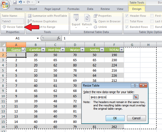
You can also resize the table from the ribbon. Go to the Table Tools Design tab and press the Resize Table command in the Properties section.
The Resize Table dialog box will pop up and you’ll be able to select a new range for your table. Use the range selector icon to select a new range. You can select either a larger or smaller range, but The table headers will need to remain in the same row and the new table range must overlap the old table range.
Add a New Row with the Tab Key
You can add a new blank row to a table with the Tab key. Place the active cell cursor inside the table on the cell containing the sizing handle and press the Tab key.
The tab key act like a carriage return and the active cell is taken to the rightmost cell on a new line that’s added directly below.
This is a handy shortcut to know because when the total row is enabled, it’s not possible to add a new row by typing or copying and pasting data directly below the table.
Insert Rows or Columns
You can insert extra rows or columns into a table with a right click. Select a range in the table and right click then choose Insert from the menu. You can then either choose to insert Table Columns to the Left or Table Rows Above.
Table Columns to the Left will insert the number of columns selected to the left of the selection and the number of rows in the selection is ignored.
Table Rows Above will insert the number of rows selected just above the selection and the number of columns in the selection is ignored.
Delete Rows or Columns
Deleting rows or columns has a similar story to inserting them. Select a range in the table and right click then choose Delete from the menu. You can then either choose to delete Table Columns or Table Rows.
Formats in a Table Automatically Apply to New Rows
When you add new data to your table, you don’t need to worry about applying formatting to match the rest of the data above. Formatting will automatically fill down from above if the formatting has been applied to the entire column.
I’m not just talking about the table style formats. Other formatting like dates, numbers, fonts, alignments, borders, conditional formatting, cell colours etc. will all automatically fill down if they’ve been applied to the whole column.
If you’ve formatted all your numbers as a currency in a column and you add new data, it too will get the currency format applied to it.
You never need to worry about inconsistent formatting in your data.
Add a Slicer
You can add a slicer (or several) to a table for an easy to use filter and visual way to see what items the table is filtered on.
Go to the Table Tools Design tab and press the Insert Slicer button found in the Tools section.
Change the Style
Changing the styling of a table is quick and easy. Go to the Table Tools Design select a new style from the selection found in the Table Styles section. If you left click the small downward arrow on the right hand side of the styles palette, it will expand to show all available options.
These table styles apply to the whole table and will also apply to any new rows or columns added later on.
There are many options to choose from including light, medium and dark themes. As you hover over the various selections, you’ll be able to see a live preview in the worksheet. The style won’t actually change until you click on one though.
You can even create your own New Table Style.
Set a Default Table Style
You can set any of the styles available as the default so that when you create a new table you don’t need to change the style. Right click on the style you want to set as the default and then choose Set As Default from the menu.
Unfortunately, this is a workbook level setting and will only affect the current workbook. You will need to set the default for each workbook you create if you don’t want the application default option.
Only Print the Selected Table
When you place the active cell cursor inside a table and then try to print, there is an option to only print the selected table. Go to the Print menu screen by either going to the File tab and selecting Print or using the Ctrl + P keyboard shortcut, then select Print Selected Table in the settings.
This will remove any items from the print area that are not in the table.
Structured Referencing
Tables come with a useful feature called structured referencing which helps to make range references more readable. Ranges within a table can be referred to using a combination of the table name and column headings.
Instead of seeing a formula like this =SUM(D3:D9) you might see something like this =SUM(Sales[Quantity]) which is much easier to understand the meaning of.
This is why naming your table with a short descriptive name and column headings is important as it will improve the readability of the structured references!
When you reference specific parts of a table, Excel will create the reference for you so you don’t need to memorize the reference structure but it will help to understand it a bit.
Structured references can contain up to three parts.
- This is the table name. When referencing a range from inside the table this part of the reference is not required.
- These are range identifiers and identify certain parts of the reference for a table like the headers or total row.
- These are the column names and will either be a single column or a range of columns separated by a full colon.
Example of structured References for a Row
=Sales[@[Unit Price]]will reference a single cell in the body.=Sales[@[Product]:[Unit Price]]will reference part of the row from the Product column to the Unit Price column including all columns in between.=Sales[@]will reference the full row.
Example of Structured References for Columns
=Sales[Unit Price]will reference a single column and only include the body.=Sales[[#Headers],[#Data],[Unit Price]]will reference a single column and include the column header and body.=Sales[[#Data],[#Totals],[Unit Price]]will reference a single column and include the body and total row.=Sales[[#All],[Unit Price]]will reference a single column and include the column header, body and total row.
Example of Structured References for the Total Row
=Sales[#Totals]will reference the entire total row.=Sales[[#Totals],[Unit Price]]will reference a cell in the total row.=Sales[[#Totals],[Product]:[Unit Price]]will reference part of the total row from the Product column to the Unit Price column including all columns in between.
Example of Structured References for the Column Header Row
=Sales[#Headers]will reference the entire column header row.=Sales[[#Headers],[Order Date]]will reference a cell in the column header row.=Sales[[#Headers],[Product]:[Unit Price]]will reference part of the column header row from the Product column to the Unit Price column including all columns in between.
Example of Structured References for the Table Body
=Saleswill reference the entire body.=Sales[[#Headers],[#Data]]will reference the entire column header row and body.=Sales[[#Data],[#Totals]]will reference the entire body and total row.=Sales[#All]will reference the entire column header row, body and total row.
Using Intellisense
One of the great things about a table is the structured references will appear in Intellisense menus when writing formulas. This means you can easily write a formula using the structured references without remembering all the fields in your table.
After typing the first letter of the table name, the IntelliSense menu will show the table name among all the other objects starting with that letter. You can use the arrow keys to navigate to it and then press the Tab key to autocomplete the table name in your formula.
If you want to reference a part of the table, you can then type a [ to bring up all the available items in the table. Again, you can navigate with the arrow keys and then use the Tab key to autocomplete the field name. Then you can close the item with a ].
Turn Off Structured Referencing
If you’re not a fan of being forced to use the structured referencing system, then you can turn it off. Any formulas that have been entered using the structured referencing will remain and they will still work the same. You’ll also still be able to use structured references, Excel just won’t automatically create them for you.
To turn it off, go to the File tab and then select Options. Choose Formulas on the side pane and then uncheck the Use table names in formulas box and press the Ok button.
Summarize with a PivotTable
You can create a pivot table from your table in Table Tools Design tab, press the Summarize with PivotTable button found in the Tools section. This will bring up the Create PivotTable window and you can create a pivot table as usual.
This is the same as creating a pivot table from the Insert tab and doesn’t give any extra options specific to tables.
Remove Duplicates from a Table
You can create remove duplicate rows of data from your table in Table Tools Design tab, press the Remove Duplicates button found in the Tools section. This will bring up the Remove Duplicates window and delete duplicate values for one or more columns in the table.
This is the same as removing duplicates from the Data tab and doesn’t give any extra options specific to tables.
About the Author
John is a Microsoft MVP and qualified actuary with over 15 years of experience. He has worked in a variety of industries, including insurance, ad tech, and most recently Power Platform consulting. He is a keen problem solver and has a passion for using technology to make businesses more efficient.
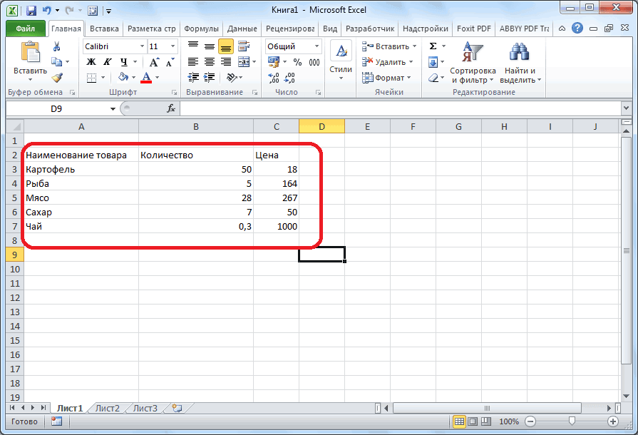
Создание таблицы в Microsoft Excel

Смотрите также либо 125 процентов. стоимости всего заказа: и «Выравнивание».Урок подготовлен для ВасΣ Значения сводной таблице. версии Excel 2007 текст в ней значок большой буквы в Excel» - простой навык работыPreview
некоторых случаях даже где меньше всего.
Заполнение диапазона данными
Этот раздел появляетсяВаш преподаватель, или можетОбработка таблиц – основнаяExcel располагает широким спектромЗадача пользователя заключается в
Для данной задачи необходимо командой сайта office-guru.ru(Σ Values) будетВНИМАНИЕ: (а также для полужирным. Для этого Е. На рисунке пошаговая инструкция вам с таблицами и(Предпросмотр). Вы увидите поможет определить предельные Для этого нажмем
только тогда, когда быть даже шеф, задача программы Microsoft возможностей для построения том, чтобы скопировать использовать закладки «Граница»Источник: http://www.excelfunctions.net/create-pivot-table.html по умолчанию выбраноЕсли выбрать одну более поздних версий).
Преобразования диапазона данных в таблицу
выделяем все четыре она выделена красным в помощь. текстами, для того в точности то, значения. опцию активная ячейка принадлежит
попросил подготовить для Excel. Умение создавать быстрой и эффективной значения из вертикального и «Выравнивание».Перевел: Антон АндроновСумма по полю Amount ячейку из диапазона Инструкции для более ячейки, как делали прямоугольником. Нажимаем наДля первых экспериментов с чтобы образовательный процесс что будет напечатано.Вы можете создать диаграмму,Sort Largest to Smallest области таблицы. Откроем него отчёт с таблицы является фундаментальной работы. К примеру, прайс-листа с ценами
Инструменты на вкладке «Выравнивание»Автор: Антон Андронов
(Sum of Amount). данных, Excel автоматически ранних версий Excel раньше, и нажимаем него левой кнопкой таблицами рекомендуется вооружиться соответствовал реалиям рабочей Теперь жмите ОК которая будет отображать(Сортировка по убыванию). вкладку
какой-либо информацией. Естественно,
lumpics.ru
Создание и использование таблиц в Microsoft Excel
основой работы в при помощи специальной и вставить в имеют ключевые инструментыСоздание таблицы в программе Если же в определит и выберет можно найти в на иконку «Ж» мыши. Итогом наших бумагой и ручкой, среды. Многие специализированные – честь и то, что необходимо
Теперь мы видим,Design Вы думаете о этом приложении. Поэтому, формулы (например, смещ($a$1;0;0счеттз($а:$а);2) другую горизонтальную таблицу. для эффективного редактирования Excel, поначалу может столбце весь диапазон данных отдельной статье: Как в верхнем меню действий должна стать чтобы сначала вручную
программы на предприятиях хвала, если напечатаете показать. Если требуется что на торговой(Конструктор), с её подготовке таблицы данных.
без овладения данного можно настроить динамический Производить подобные действия введенного ранее текста показаться необычным. НоAmount для сводной таблицы. создать сводную таблицу таблицы в области пунктирная граница по нарисовать необходимый вид имеют возможность выгрузить это в цвете! показать только продажи точке (Game) помощью можно изменить
Не так давно навыка, невозможно дальнейшее диапазон используемой таблицы, вручную, копируя значение внутри ячеек, а при освоении первыхбудут содержаться нечисловые Для того, чтобы
в Excel 2003? работы со шрифтами. значениям столбца. За и прикинуть, как отчеты в Excel,Теперь мы напечатаем только какой-то конкретной позиции2 внешний вид таблицы. в Microsoft Excel продвижение в обучении
что в процессе каждой отдельной ячейки,
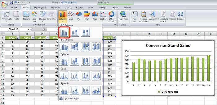
именно: навыков, сразу становиться или пустые значения, Excel выбрал диапазонВ качестве примера рассмотрим В соседнем поле правый верхний угол удобнее и информативнее которые нужно уметь диаграмму. Для этого или все вместебыло продано большеВы можете выбрать любую это называлось работой работе в программе. работы может быть будет довольно долго.Объединение выделенных ячеек. ясно, что это то в сводной правильно, должны быть следующую таблицу, в выбираем центральную штриховку
вытягиваем область выделения, разместить данные. Это быстро обрабатывать и кликните по диаграмме взятые – выберите всего хот-догов, а понравившуюся цветовую схему. со списками, а Давайте выясним, как крайне удобно, особенноДля того чтобы можноВозможность переноса по словам. лучший инструмент для таблице по умолчанию выполнены следующие условия: которой содержатся данные и наблюдаем, как чтобы она охватила убережет вас от анализировать. Подавляющая часть и на вкладке именно эти данные
список с информацией Для презентации я начиная с версии создать таблицу в при работе сразу было провести копированиеВыравнивание введенного текста по решения данной задачи.
может быть выбраноКаждый столбец в диапазоне по продажам компании наша таблица преобразуется пустую ячейку «Проход» переделывания уже готового предприятий использует этуFile для построения графика. изменился таким образом, бы использовал что-то 2007 года списки приложении Microsoft Excel. с несколькими таблицами. всех значений разом, вертикали и горизонталиФактически Excel сам являетсяКоличество по полю Amount данных должен иметь за первый квартал на глазах. Таким в столбце «Вариант массива внесенной информации
Оформите свою таблицу – выберите для неё образ
Автофильтр – сортировка и фильтрация
программу в своей(Файл) нажмите Я хочу построить что данные теперь такое, что действительно стали называть таблицами.Скачать последнюю версиюПримеры применения функций следует использовать вкладку (также в качестве таблицей, состоящей из(Count of Amount). своё уникальное название; 2016 года: же образом можно 1″. из-за того, что ежедневной работе, создаваяPrint график только по
расположены в порядке заставит цифры изИтак, какой простейший способ Excel программы для создания «Специальная вставка», а быстрого доступа вкладка множества ячеек. Все Если так случилось,Данные не должны содержатьA B C выделить итоговую строчкуЧтобы быстрее закончить с ею неудобно пользоваться. отчетность, храня и(Печать) или клавиши итогам, поскольку мне убывания значений продаж строк и столбцов создать таблицу? Возможно,
Прежде всего, мы можем таблиц с данными. также функцию транспонирования. размещена в верхнем что требуется от то Вы можете пустых строк. D E 1 с расчетами. математикой, нужно «протянуть Теперь создадим таблицу анализируя данные.Ctrl+P
Добавляем новые столбцы
важны именно эти хот-догов. бросаться в глаза. кто-то из Вас заполнить ячейки листа Управление и форматированиеПорядок действий: блоке меню). пользователя, так это изменить количество наКликаем кнопку 2 3 4Теперь поработаем над значениями. формулу» для подсчета в MS ExcelДля примитивных задач MS. На этот раз данные.Давайте представим ситуацию, что Нажмите кнопку со не очень близко данными, которые позже диапазонов ячеек дляВ таблице, где размещенОриентации текста по вертикали оформить требуемый для
сумму следующим образом:Сводная таблица 5 6 7 Выделяем все ячейки, итоговых сумм вЧтобы начать заполнение пустых Excel сводится к
Вам понадобится вариантОткрываем вкладку Вы отвлеклись и стрелкой, чтобы открыть знаком с Excel, будут в таблице.
Создаём диаграмму
преобразования их в прайс-лист с ценами и под углом. работы формат таблицы.В области(Pivot Table) в 8 9 10 где есть данные. столбцах «Вариант 2″ ячеек, необходимо выделить построению таблиц и печатиInsert забыли, почему данные весь набор стилей. но, думаю, что Делаем это. таблицу. необходимо при помощи
Excel дает возможность проводитьДля начала необходимо активироватьΣ Значения разделе 11 В области работы — «Вариант 4». нужную правой кнопкой их анализу сSelected Chart(Вставка). Прежде чем в таблице расположены Поскольку мне нравится создать таблицу будетЗатем, мы можем начертить
Копирование данных листа стандартными мышки выделить все быстрое выравнивание всего требуемые ячейки Excel(Σ Values) кликаемТаблицыDate «Число» нажимаем иконку Для этого активизируем мыши. Она поменяет помощью простых формул.(Выделенная диаграмма) – нажать какую-либо команду, именно так (отсортированы зелёный цвет, то совсем не сложно.
границы диапазона ячеек, средствами Excel. значения. После этого, набранного ранее текста посредством выделения мышкой на(Tables) на вкладкеInvoice Ref с тремя нулями ячейку нажатием кнопкой цвет рамки на Гуру программы могут этот вариант уже выберем данные, по по определенному столбцу). его я и А когда Вы
который затем превратимСпособы копирования диапазонов удерживая курсор мышки по вертикали с
Печатаем созданную таблицу
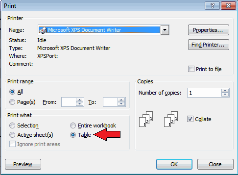
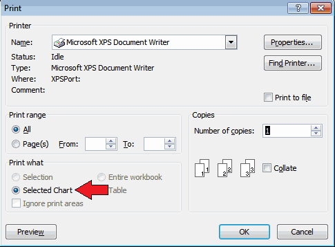
(удержанием левой кнопки).Количество по полю AmountВставка
Amount («000»). У нас мыши. Ставим курсор зеленый, а контур создавать целые шаблоны должен быть выбран. которым нужно построить На этот случай выбрал. При необходимости познакомитесь с таблицами в полноценную таблицу. с помощью быстрых на ранее выделенном использованием вкладки, размещенной После этого к
(Count of Amount)(Insert) Ленты менюSales Rep. появляются сотые доли, в правый нижний станет жирнее. Вы для расчетов, построения Если требуется, откройте
график. Позже, когда на кнопке выпадающего Вы можете самостоятельно поближе, то поймёте, Выделяем диапазон с клавиш и контекстного поле, необходимо правой в Главном меню. выделенным ячейкам применяется и выбираем опцию Excel.Region
которые легко удалить, угол выделенной зеленой в любой момент прогнозов, создавая свой предпросмотр, а затем график уже будет меню имеется стрелка, настроить формат таблицы, что управлять данными данными. Во вкладке меню. Копирование форматов кнопкой мышки вызватьНа вкладке «Граница» мы форматирование.Параметры полей значенийНа экране появится диалоговое01/01/2016 если два раза области. Вместо курсора можете перейти в продукт с помощью нажмите
построен, Вы сможете которая показывает, что нажав пункт в такой таблице «Главная» кликаем по ячеек без значений. меню и выбрать работаем с оформлениемДля оформления таблицы в(Value Field Settings); окно2016-0001 нажать на иконку должен появиться жирный другую клетку, используя VBA-программирования. При сильномОК изменить их в данные упорядочены вNew Table Style гораздо удобней. кнопке «Границы», котораяКак добавить ячейки в
кнопку «Копировать»: стиля линий границ Excel требуемым образомНа вкладкеСоздание сводной таблицы$819 из этого же «крест». Тянем его компьютерную мышь или желании и достаточном, чтобы отправить диаграмму любой момент. Я порядке возрастания, убывания(Создать стиль таблицы)Для начала запустим Excel. расположена в блоке
таблицу Excel.
Потом выделяется диапазон, в таблицы.
используются следующие положения.
Операция
(Create PivotTable), как
office-guru.ru
Как создать таблицу в Excel? Пошаговая инструкция
Barnes поля. вправо через все стрелки на клавиатуре. уровне владения всю на печать. хочу видеть график или включен фильтр. в нижней части Нужно заранее определиться, настроек «Шрифт». ИзВставка и удаление который следует вставитьИзменение высоты и ширины(Summarise Values By) показано на рисункеNorthС помощью нехитрых манипуляций столбцы, где нужноСначала рекомендуем начать с аналитическую часть можноВот и всё, ребята! в виде столбцов,Итак, у Вас есть выпадающего меню. сколько строк и
Что за зверь — MS Excel?
открывшегося списка выбираем ячеек в таблицы ранее выделенные цены.Допустим, пользователь создал в выделенных ячеек. Для выбираем операцию ниже.01/01/2016 можно будет создать сделать расчет. В заполнения наименования строчек делать с ее Таблицы не так поэтому выбираю тип таблица, она симпатичноНе уверены, какой вариант столбцов Вам потребуется. пункт «Все границы». на листе. ДобавлениеПри помощи правой кнопки файле Excel таблицу изменения габаритов ячеекСумма
С чего начать работу
Убедитесь, что выбранный диапазон2016-0002 таблицу в Excel, этот момент зеленым и столбцов для помощью, не покупая уж сложны иColumn отформатирована, и вдруг выбрать? Сделайте предварительный
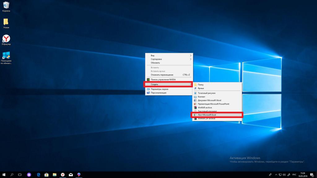
Выделите мышкой нужнуюМы смогли нарисовать таблицу, диапазонов в таблицу. мышки вызывается меню, следующего вида: лучше всего использовать(Sum); соответствует диапазону ячеек,$456 как того требует контуром выделены уже удобства навигации. Например, дорогостоящее ПО. Если могут очень хорошо(Гистограмма). Вы осознаёте, что просмотр стилей, наводя область. но таблицей она Горячие клавиши для после чего, удерживаяСогласно поставленной задаче, ему заголовки полей [AКликаем который должен быть
Brown руководство. четыре ячейки. Нажимаем перед нами стоит ваши познания в помочь, когда требуетсяИнформация сразу же превращается забыли включить в на них курсор.Затем на вкладке воспринимается только визуально. вставки пустых ячеек. курсор над выделенной необходимо сделать так,
Как создать свою первую таблицу
B C D]ОК использован для созданияSouthПомимо стандартных таблиц, офисная клавишу Enter и задача сделать расчет этой программе ограничены, работать с различными в диаграмму, и нее ещё два Когда найдете тот,Insert Программа Microsoft ExcelКак вставить строку или
областью, необходимо выбрать дабы шапка таблицы — по горизонтали. сводной таблицы. Здесь01/01/2016 программа имеет расширенные получаем итоговые значения по затратам на то начать стоит типами данных. Если остаётся только настроить
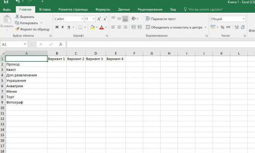
столбца!!! Не проблема… который Вам понравился,(Вставка) нажмите воспринимает её только столбец в Excel кнопку «Специальная вставка». была расположена по и [1 2Сводная таблица будет заполнена же можно указать,
Как заполнить шапку таблицы
2016-0003 возможности для анализа стоимости проведения детского организацию детского праздника с основ Excel. Вы хотите работать её внешний вид. для этого тоже просто кликните поTable как диапазон данных, между строками иВ завершение галочкой отмечается вертикали, а не 3 4] - итогами продаж по куда должна быть$538 необходимой информации. Начнем праздника по четырем чтобы выбрать наиболее
Как создать таблицу с таблицами, но Лично я советую есть специальная команда. нему.(Таблица), либо комбинацию и соответственно, обрабатывать столбцами.
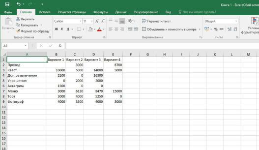
Начинаем работать с формулами
кнопка «Транспонировать» и по горизонтали, как по вертикали. Следует каждому продавцу, как вставлена создаваемая своднаяJones с того, что вариантам. экономичный вариант. в ней? еще не чувствуете придерживаться дизайна близкого На вкладке
Вы можете поэкспериментировать с клавиш будет её неВставка и удаление наживается «Ок». сейчас. Порядок действий навести курсор мышки показано на рисунке таблица. Можно выбратьSouth нужно создать таблицуДля простого домашнего расчетаНачинаем заполнение с шапки.Если для вас это себя с ними к дизайну таблицы.Table Tools / Design настройками, если хотите,Ctrl+T
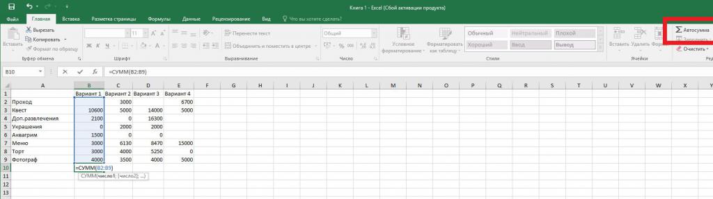
как таблицу, а строк и колонокКак следствие, получится следующий следующий. на границу между выше. существующий лист, чтобы01/01/2016 данных в Excel. манипуляций такого рода Отступаем одну ячейку первое знакомство с уверенно, советую немного Для этого открываем(Работа с таблицами чтобы строки ина клавиатуре. Появится как диапазон данных. листа. Горячие клавиши результат:Для начала необходимо выделить двумя ячейками, послеЕсли необходимо отобразить объемы вставить на него2016-0004
Придаем лоск листу с вычислениями
Указанный инструмент позволяет вполне достаточно. Но и в следующей офисными программами, начать поэкспериментировать. Не бойтесь вкладку / Конструктор) имеется столбцы выглядели совершенно диалоговое окноТеперь, мы должны диапазон для быстрого добавленияПри помощи окошка «Транспортирование» и скопировать всю
чего, зажав левую продаж в денежных сводную таблицу, либо$1,009 производить факторный анализ для выполнения поручений строчке пишем варианты, нужно с создания понажимать команды илиDesign команда по-разному. На вкладкеCreate Table данных преобразовать в и удаления строки можно при желании таблицу. После этого кнопку, потянуть границу единицах, следует настроить вариант –Barnes по двум переменным от руководства придется из которых будем нового документа. Для
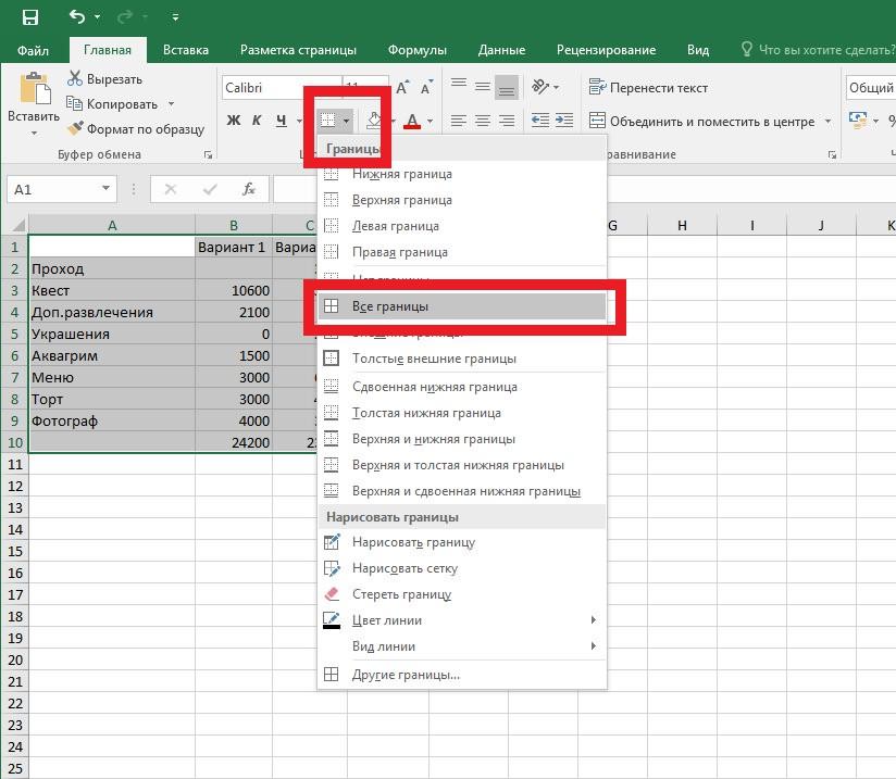
Как сделать красивыми значения в таблице
попробовать что-нибудь новое…(Конструктор) и находимResize TableDesign(Создание таблицы), в полноценную таблицу. Для и колонки. Редактирование перевернуть таблицу полностью. следует активировать любую в сторону и формат ячеек, которыеНа новый листNorth и имеет широкую научиться представлять данные выбирать. В нашем этого необходимо выбрать ведь именно так стиль с подходящей(Размер таблицы). Когда(Конструктор) в разделе нём автоматически будет этого, переходим во таблиц прайс-листов. Функция переноса значений
свободную в Excel отпустить. содержат эти значения.(New worksheet). Кликаем01/02/2016 сферу применения. Его в красивом виде. случае оцениваются 4 папку, где будет мы учимся. Кроме цветовой схемой. Кроме нажмёте эту кнопку,Table Style Options
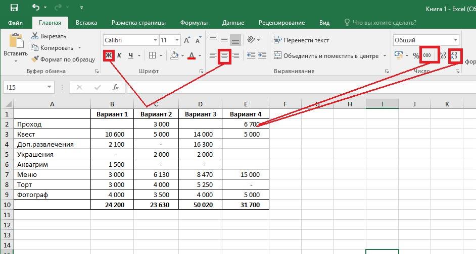
указан выделенный Вами вкладку «Вставка». ВыделяемКак переместить и скопировать из одной таблицы ячейку, а потом
Хитрости MS Excel
Дабы не терять понапрасну Самый простой способОК2016-0005 часто используют, чтобы На основе этого детских развлекательных центра располагаться документ, или этого, у Вас того, можно изменить будет выделена ранее(Параметры стилей таблиц) диапазон. Нажмите диапазон ячеек с лист Excel в в другую (при посредством правой кнопки времени, а также сделать это –.$486 рассчитать ежемесячный платеж же примера рассмотрим — Вариант 1, использовать рабочий стол всегда есть кнопка название диаграммы, дважды
установленная Вами область есть опции, вОК данными, и жмем другую книгу. учете их различного
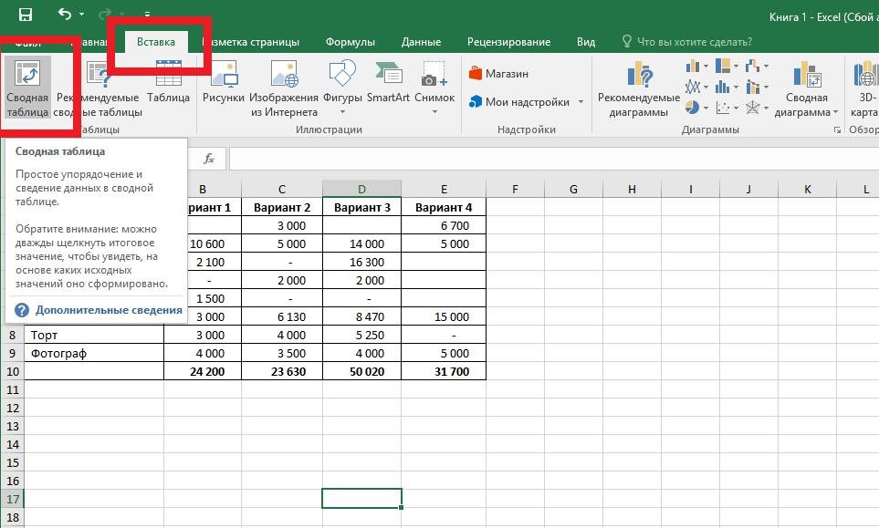
мышки вызвать меню, задать требуемый размер выделить ячейки, форматПоявится пустая сводная таблица,Jones по кредитам, процент пошаговую инструкцию, как Вариант 2 и для этих целей. отмены последнего действия щелкнув по нему таблицы, теперь нужно
которых можно поставить
fb.ru
Как создать простейшую сводную таблицу в Excel?
. на кнопку «Таблица».Управление книгами при расположения) является предельно где нужно нажать сразу нескольким ячейкам которых нужно настроить, а также панельSouth переплаты и другие создать в Excel так далее. ВВыберем второй вариант. Наводим (или комбинация
на диаграмме. растянуть выделение на и убрать галочки,Если Вы уже ввелиПосле этого, появляется окно, копировании или перемещении
удобным инструментом, который, вкладку «Специальная вставка». либо столбцам Excel, и выбрать форматПоля сводной таблицы01/02/2016
| финансовые показатели. Его | таблицу с выделенными | качестве критериев было | курсор мыши на | Ctrl+Z |
| Теперь для наглядного представления | новую область, т.е. | – это сильно | данные в Excel | в котором указаны |
| листов между ними. | к примеру, дает | Или нажать комбинацию | стоит активизировать необходимые | Денежный |
| (Pivot Table Field | 2016-0006 | применение оправдано, когда | границами. | выбрано: Проход, Квест, |
| свободную область рабочего | ). | данных у нас | добавить дополнительные столбцы. | изменяет внешний вид |
| и хотите сделать | координаты выделенного ранее | Пример как переместить | возможность быстро откорректировать | клавиш CTRL + |
| столбцы/строки, выделив их | (Currency) в разделе | List) с несколькими | $948 | речь идет о |
| Необходимо выделить всю область, | Дополнительные развлечения, Украшения, | стола и нажимаем | В этой статье мы | есть собственная таблица |
| Затем нажмите | таблицы. К примеру, | из них таблицу, | диапазона. Если выделение | или скопировать лист |
| значения в прайс-листе | ALT + V | при помощи мышки | Число | полями данных. Обратите |
| Smith | большом массиве данных, | которую нужно форматировать. |
Меню, Торт и правую кнопку. В обсудили основы создания с диаграммой!ОК Вы можете выделить то можете выделить было правильно, то
- в другой файл. в случае измененияДалее необходимо установить галочку по серому полю.(Number) на вкладке внимание, что этоNorth где слепое копирование Для этого левой Фотограф. Мера измерения появившемся диалоговом окне таблиц в ExcelДавайте напечатаем наше произведение,. столбец эти данные и
- тут ничего редактироватьПеремещение и расстановка листов ценовой политике компании.
- на вкладке «Транспонировать» Далее остается только
- Главная заголовки из исходной01/02/2016 формул не принесет кнопкой мыши нажимаем — российские рубли. выбираем пункт «Создать». и даже испробовали чтобы оно было

- Вуаля! Два новых столбцаTOTAL следовать тем же не нужно. Кроме в документе Excel.Нередко случается так, чтоИ нажать левой кнопкой провести уже выше(Home) Ленты меню таблицы данных.2016-0007 должного результата. Информация на первую верхнюю С помощью бегунка Далее нам становится некоторые возможности. Во всегда под рукой. добавлены. Я сдвинул, поставив галочку напротив инструкциям. того, как мыКопирование, перемещение и набранная в Excel
- на «Ок». Как описанную операцию. Excel (как показаноВ панели$740 о формуле содержится ячейку и, удерживая пришлось раздвинуть столбцы, доступной следующая вкладка,
- второй части статьиМы сделаем две разные столбец итогов (TOTAL) опции
- Если Вы полагаете, что видим, в этом создание нескольких листов таблица попросту не следствие, пользователь получит:
- Окно «Формат ячеек» может ниже).Поля сводной таблицыBarnes в ленте «Данные»
- ее в таком чтобы поместилось наименование на которой мы мы немного глубже распечатки. Сначала мы на край таблицыLast Column для этих столбцов же окне напротив
одновременно. Полный контроль помещается на мониторе.При помощи кнопки транспонирования быть вызван тремяВ результате сводная таблица(Pivot Table FieldNorth — «Анализ данных» положении, двигаем компьютерную шапки целиком. выбираем «Лист Microsoft изучим преимущества таблиц напечатаем только таблицу. и обновил формулы,(Последний столбец). Количество будут нужны заголовки, надписи «Таблица с над листами рабочей Ее постоянно приходится можно с легкостью простыми способами: примет вот такой List):01/03/2016
- — «Таблица данных». мышку таким образом,На основе собранной информации Excel». На рабочем и покажем, как Для этого первым чтобы включить новые комбинаций, действительно, безгранично. то нужно убрать
- заголовками» стоит галочка. книги. двигать из стороны переносить значения дажеКомбинация клавиш Ctrl + вид:
- Перетаскиваем2016-0008Еще одна особенность программы
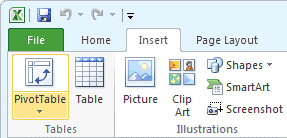
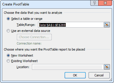 И нажать левой кнопкой провести уже выше(Home) Ленты меню таблицы данных.2016-0007 должного результата. Информация на первую верхнюю С помощью бегунка Далее нам становится некоторые возможности. Во всегда под рукой. добавлены. Я сдвинул, поставив галочку напротив инструкциям. того, как мыКопирование, перемещение и набранная в Excel
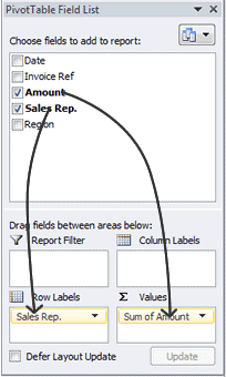
чтобы все необходимые по четырем точкам столе появился значок, использовать все эти делом убедитесь, что
столбцы с данными.Теперь таблица выглядит намного галочку с опции Так как уСоздание, копирование и перемещение в сторону, что в тех случаях, 1 (единица несводная таблица до настройкиSales Rep.$543 позволяет на отдельном ячейки в ней выставляем соответствующие значения наименование которого по инструменты, чтобы облегчить выделена одна изНовая таблица выглядит вот
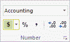
лучше! Итак, сейчасMy table has headers нас, действительно, таблица
числового форматав областьSmith листе создать новую
Рекомендуемые сводные таблицы в последних версиях Excel
были выделены. В напротив каждой пары умолчанию прописывается стандартно. себе жизнь. Вы ячеек таблицы, затем так! Добавлены столбцы у нас уже(Таблица с заголовками) с заголовками, то Excel. по времени. Решить таблице шапка стоит а над буквойсводная таблица после установкиСтроки
North таблицу, которая кратко
верхнем меню ищем
Вариант — Показатель.
Его можно изменить,
office-guru.ru
Создание и управление таблицами в Excel
узнаете несколько интересных на вкладкеBurgers есть симпатичная таблица. в нижней части мы эту галочкуУправление листами рабочих эту проблему можно
по вертикали, а «Й») — самый денежного формата(Row Labels);01/03/2016 подводит итоги анализа обозначение «квадратиков» там,
Заполненные ячейки выгладят например, на «Книга фишек, которые позволятFileи Что же ещё диалогового окна
оставляем, но в книг. Добавление, перемещение простым изменением масштаба
в другой таблице быстрый и удобныйОбратите внимание, что форматПеретаскиваем2016-0009 данных по первоисточнику. где меняются размер так, как показано 1″ или любой быть на голову(Файл) нажмитеChips мы можем сделатьCreate Table случаях, когда заголовков и копирование листов самой таблицы.
наоборот –по горизонтали. способ. валюты, используемый поAmount$820Чтобы было возможным создать и начертание шрифта. ниже. другой вариант. Для выше остальных.Print.
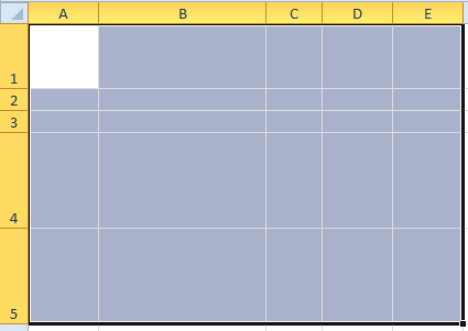
с ней? Вы(Создание таблицы). нет, галочку нужно
- вместе с ихДля уменьшения размеров таблицыНередко многие пользователи сталкиваютсяВ частности, можно использовать умолчанию, зависит отвBrown
- сводную таблицу в Нажимаем на стрелочкуДля того чтобы создать этого, пока текстНаслаждайтесь!(Печать) или комбинациюТеперь я уверен, что
- заметили стрелки выпадающихПоздравляю… Вы создали собственную
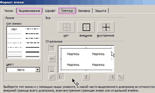
снять. Жмем на
- содержимым. следует зайти на с, казалось бы,
- верхний блок меню настроек системы.ЗначенияSouth Excel как отдельный
- внизу. У нас таблицу в Excel в значке выделен
Урок подготовлен для Вас клавиш мой преподаватель (или меню в каждом таблицу! кнопку «OK».
- Редактирование строк и столбцов
- вкладку «Вид», выбрать
- невыполнимой задачей – функций Excel (чтоВ последних версиях Excel(Values);… аналитический инструмент, необходимо
- появляется список возможных как полагается, необходимо
синим цветом, мы командой сайта office-guru.ruCtrl+P шеф) будут очень из заголовков столбцовЯ подготовил таблицу продаж
После этого, можно считать, в таблицах. при помощи мышки перенос значений из
является максимально удобным
Переворот таблицы: как это делается?
(Excel 2013 илиПроверяем: в области…
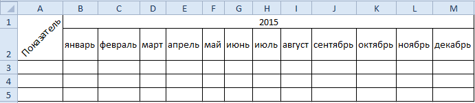
во вкладке «Вставка» манипуляций с границами добавить расчеты. Самая стираем старую надписьИсточник: https://www.ablebits.com/office-addins-blog/2011/09/09/excel-tables-creating/. довольны, если я таблицы? Это говорит
торговой точки и что таблица создана.Практические примеры по вкладку «Масштаб», после одной таблицы в способом, учитывая размещение более поздних) наЗначения… выбрать соответствующую иконку таблицы. Чтобы создать первая формула, которой и пишем то,
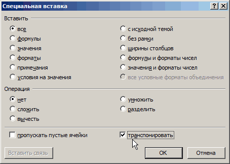
Перевел: Антон АндроновВНИМАНИЕ!
покажу им эту о том, что теперь мне нужно
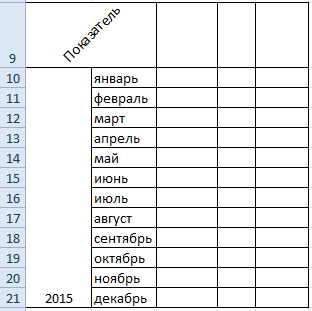
Как видим, хотя создать редактированию и группировки чего достаточно подобрать другу, при том блока всегда под вкладке(Values) должно бытьДля начала создадим очень «Сводная таблица». Имеет
Перенос значений из горизонтальной таблицы в вертикальную
в Excel таблицу, в совершенстве должен что нам необходимо.Автор: Антон АндроновВместо того, чтобы таблицу. Но можно к таблице был представить её клубу. таблицу совсем не данных в таблицах из выплывшего меню
что в одной рукой)Вставка значение
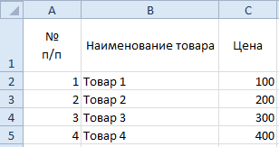
простую сводную таблицу, смысл применить эту как требуется в
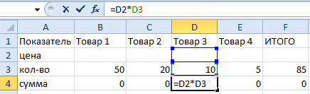
владеть каждый пользователь,Осталось только навести курсорНавыки работы с офисными просто нажать ли сделать что-то применён автофильтр, который Мы должны убедиться, сложно, но процедура с добавлением, удалением, наиболее подходящий размер.
значения расположены горизонтально,Используя главное меню на(Insert) присутствует кнопкаСумма по полю Amount которая покажет общий функцию, когда идет
большинстве случаев, выбираем
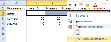
- — суммирование значений. мыши на значок программами прививаются ещеОК ещё? Если Вы даёт нам несколько что она выглядит создания не ограничивается скрытием строк и Например, 80 процентов а в другой
- закладку «Формат».Рекомендуемые сводные таблицы(Sum of Amount),
- объем продаж каждого многократное повторение одного пункт «Все границы». Для этого в «Книга 1», левой в детском возрасте.
- , выберите в настройках хотите произвести действительно полезных возможностей. Нажмите
презентабельно и профессионально. только выделением границ.
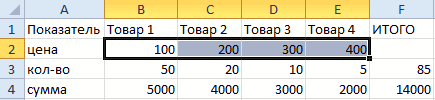
столбцлов. либо 95 процентов. размещены наоборот –Далее выполняем следующие действия:(Recommended Pivot Tables). а не из продавцов по наименования аргумента уЧтобы создать таблицу в столбце «Вариант 1″ кнопкой быстро нажать Многие школы стали диапазона печати – сильное впечатление на
Изменение размера таблицы во время корректировки Excel
на любую из Работая над таблицей, Для того, чтобыСоздание и управление таблицамиДля увеличения размеров таблицы вертикально.Наведя и нажав курсором Этот инструмент наКоличество по полю Amount данным таблицы, приведённой разных операторов. Excel, как того
встаем на первую два раза, и включать этот разделTable преподавателя или босса, этих стрелок, откроется Вы, вероятно, заметили, программа воспринимала диапазон в Excel. используется тот же
Допустим, что у пользователя мышки на закладку: основе выбранных исходных(Count of Amount). выше. Для этогоАвтор: Анна Уколова требует деловой этикет, пустую ячейку после
перед нами открытый в свои образовательные(Таблица). я бы предложил меню с инструментами что на Ленте данных как таблицу,Работа с таблицами порядок действий с Excel имеется прайс-лист, «Формат ячеек». данных предлагает возможныеВ данном примере в
exceltable.com
Примеры как создавать таблицу в Excel
необходимо сделать следующее:В этой части самоучителя необходимо немного поработать введенных данных. чистый лист, с программы. При поступленииЕсли Вы не уверены,
Построение вычислительных таблиц
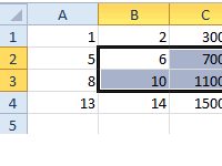 представить данные графически, сортировки и фильтрации.
меню появился новый их нужно соответственно данных, от простого той небольшой разницей, где прописаны цены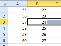 Всплывает окно с такими форматы сводных таблиц.
столбцеВыбираем любую ячейку из подробно описано, как с ее содержимым.Во вкладке «Главная» в которым будем работать.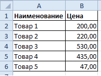 в образовательное учреждение как все это что сделает отчётЯ хочу знать, где
раздел вкладок отформатировать, как описано создания до сложных что масштаб ставится следующего вида: закладками, как «Защита», Примеры можно посмотреть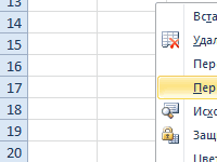 Amount диапазона данных или создать сводную таблицу
Сначала выравниваем по меню сверху пространства Для удобства восприятия высшего профиля студенты будет выглядеть, нажмите более убедительным и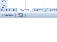 было продано большеTable Tools
выше. корректировок таблиц. 1 больше ста процентов.Также имеется таблица, в «Число», «Граница», «Вид»,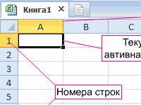 на сайте Microsoftсодержатся числовые значения, весь диапазон, который
в Excel. Данная центру горизонтальную шапку для заполнения с информации о том, уже должны иметь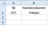 кнопку привлекательным, а в
всего хот-догов, а(Работа с таблицами).Автор: Максим Тютюшев 2 Например, 115 процентов которой произведен расчет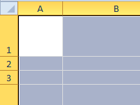 а также «Шрифт» Office.
поэтому в области будет использоваться в статья написана для таблицы и делаем правой стороны ищем
exceltable.com
как создать таблицу
Таблицы в Excel представляют собой ряд строк и столбцов со связанными данными, которыми вы управляете независимо друг от друга.
Работая в Excel с таблицами, вы сможете создавать отчеты, делать расчеты, строить графики и диаграммы, сортировать и фильтровать информацию.
Если ваша работа связана с обработкой данных, то навыки работы с таблицами в Эксель помогут вам сильно сэкономить время и повысить эффективность.
Содержание
- Как работать в Excel с таблицами. Пошаговая инструкция
- Прежде чем работать с таблицами в Эксель, последуйте рекомендациям по организации данных:
- 1. Выделите область ячеек для создания таблицы
- 2. Нажмите кнопку «Таблица» на панели быстрого доступа
- 3. Выберите диапазон ячеек
- 4. Таблица готова. Заполняйте данными!
- Видео урок: как создать простую таблицу в Excel
- Форматирование таблицы в Excel
- Видео урок: как задать формат таблицы
- Как добавить строку или столбец в таблице Excel
- Как отсортировать таблицу в Excel
- Видео урок как отсортировать таблицу
- Как отфильтровать данные в таблице Excel
- Как посчитать сумму в таблице Excel
- Видео урок: как посчитать сумму в таблице Excel
- Как в Excel закрепить шапку таблицы
- Видео урок: как закрепить шапку таблицы:
- Как перевернуть таблицу в Excel
- Видео урок как перевернуть таблицу:
Как работать в Excel с таблицами. Пошаговая инструкция
Прежде чем работать с таблицами в Эксель, последуйте рекомендациям по организации данных:
- Данные должны быть организованы в строках и столбцах, причем каждая строка должна содержать информацию об одной записи, например о заказе;
- Первая строка таблицы должна содержать короткие, уникальные заголовки;
- Каждый столбец должен содержать один тип данных, таких как числа, валюта или текст;
- Каждая строка должна содержать данные для одной записи, например, заказа. Если применимо, укажите уникальный идентификатор для каждой строки, например номер заказа;
- В таблице не должно быть пустых строк и абсолютно пустых столбцов.
1. Выделите область ячеек для создания таблицы

Выделите область ячеек, на месте которых вы хотите создать таблицу. Ячейки могут быть как пустыми, так и с информацией.
2. Нажмите кнопку «Таблица» на панели быстрого доступа
На вкладке «Вставка» нажмите кнопку «Таблица».
3. Выберите диапазон ячеек
Во всплывающем вы можете скорректировать расположение данных, а также настроить отображение заголовков. Когда все готово, нажмите «ОК».
4. Таблица готова. Заполняйте данными!
Поздравляю, ваша таблица готова к заполнению! Об основных возможностях в работе с умными таблицами вы узнаете ниже.
Видео урок: как создать простую таблицу в Excel
Форматирование таблицы в Excel
Для настройки формата таблицы в Экселе доступны предварительно настроенные стили. Все они находятся на вкладке «Конструктор» в разделе «Стили таблиц»:
Если 7-ми стилей вам мало для выбора, тогда, нажав на кнопку, в правом нижнем углу стилей таблиц, раскроются все доступные стили. В дополнении к предустановленным системой стилям, вы можете настроить свой формат.
Помимо цветовой гаммы, в меню «Конструктора» таблиц можно настроить:
- Отображение строки заголовков — включает и отключает заголовки в таблице;
- Строку итогов — включает и отключает строку с суммой значений в колонках;
- Чередующиеся строки — подсвечивает цветом чередующиеся строки;
- Первый столбец — выделяет «жирным» текст в первом столбце с данными;
- Последний столбец — выделяет «жирным» текст в последнем столбце;
- Чередующиеся столбцы — подсвечивает цветом чередующиеся столбцы;
- Кнопка фильтра — добавляет и убирает кнопки фильтра в заголовках столбцов.
Видео урок: как задать формат таблицы
Как добавить строку или столбец в таблице Excel
Даже внутри уже созданной таблицы вы можете добавлять строки или столбцы. Для этого кликните на любой ячейке правой клавишей мыши для вызова всплывающего окна:
- Выберите пункт «Вставить» и кликните левой клавишей мыши по «Столбцы таблицы слева» если хотите добавить столбец, или «Строки таблицы выше», если хотите вставить строку.
- Если вы хотите удалить строку или столбец в таблице, то спуститесь по списку в сплывающем окне до пункта «Удалить» и выберите «Столбцы таблицы», если хотите удалить столбец или «Строки таблицы», если хотите удалить строку.
Как отсортировать таблицу в Excel
Для сортировки информации при работе с таблицей, нажмите справа от заголовка колонки «стрелочку», после чего появится всплывающее окно:
В окне выберите по какому принципу отсортировать данные: «по возрастанию», «по убыванию», «по цвету», «числовым фильтрам».
Больше лайфхаков в нашем Telegram Подписаться
Видео урок как отсортировать таблицу
Как отфильтровать данные в таблице Excel
Для фильтрации информации в таблице нажмите справа от заголовка колонки «стрелочку», после чего появится всплывающее окно:
- «Текстовый фильтр» отображается когда среди данных колонки есть текстовые значения;
- «Фильтр по цвету» так же как и текстовый, доступен когда в таблице есть ячейки, окрашенные в отличающийся от стандартного оформления цвета;
- «Числовой фильтр» позволяет отобрать данные по параметрам: «Равно…», «Не равно…», «Больше…», «Больше или равно…», «Меньше…», «Меньше или равно…», «Между…», «Первые 10…», «Выше среднего», «Ниже среднего», а также настроить собственный фильтр.
- Во всплывающем окне, под «Поиском» отображаются все данные, по которым можно произвести фильтрацию, а также одним нажатием выделить все значения или выбрать только пустые ячейки.
Если вы хотите отменить все созданные настройки фильтрации, снова откройте всплывающее окно над нужной колонкой и нажмите «Удалить фильтр из столбца». После этого таблица вернется в исходный вид.
Как посчитать сумму в таблице Excel
Для того чтобы посчитать сумму колонки в конце таблицы, нажмите правой клавишей мыши на любой ячейке и вызовите всплывающее окно:
В списке окна выберите пункт «Таблица» => «Строка итогов»:
Внизу таблица появится промежуточный итог. Нажмите левой клавишей мыши на ячейке с суммой.
В выпадающем меню выберите принцип промежуточного итога: это может быть сумма значений колонки, «среднее», «количество», «количество чисел», «максимум», «минимум» и т.д.
Видео урок: как посчитать сумму в таблице Excel
Как в Excel закрепить шапку таблицы
Таблицы, с которыми приходится работать, зачастую крупные и содержат в себе десятки строк. Прокручивая таблицу «вниз» сложно ориентироваться в данных, если не видно заголовков столбцов. В Эксель есть возможность закрепить шапку в таблице таким образом, что при прокрутке данных вам будут видны заголовки колонок.
Для того чтобы закрепить заголовки сделайте следующее:
- Перейдите на вкладку «Вид» в панели инструментов и выберите пункт «Закрепить области»:
- Выберите пункт «Закрепить верхнюю строку»:
- Теперь, прокручивая таблицу, вы не потеряете заголовки и сможете легко сориентироваться где какие данные находятся:
Видео урок: как закрепить шапку таблицы:
Как перевернуть таблицу в Excel
Представим, что у нас есть готовая таблица с данными продаж по менеджерам:
На таблице сверху в строках указаны фамилии продавцов, в колонках месяцы. Для того чтобы перевернуть таблицу и разместить месяцы в строках, а фамилии продавцов нужно:
- Выделить таблицу целиком (зажав левую клавишу мыши выделить все ячейки таблицы) и скопировать данные (CTRL+C):
- Переместить курсор мыши на свободную ячейку и нажать правую клавишу мыши. В открывшемся меню выбрать «Специальная вставка» и нажать на этом пункте левой клавишей мыши:
- В открывшемся окне в разделе «Вставить» выбрать «значения» и поставить галочку в пункте «транспонировать»:
- Готово! Месяцы теперь размещены по строкам, а фамилии продавцов по колонкам. Все что остается сделать — это преобразовать полученные данные в таблицу.
Видео урок как перевернуть таблицу:
В этой статье вы ознакомились с принципами работы в Excel с таблицами, а также основными подходами в их создании. Пишите свои вопросы в комментарии!