
When we need to collect data from others, they may write different things from their perspective. Still, we need to make all the related stories under one. Also, it is common that while entering the data, they make mistakes because of typo errors. For example, assume in certain cells, if we ask users to enter either “YES” or “NO,” one will enter “Y,” someone will insert “YES” like this, and we may end up getting a different kind of results. So in such cases, creating a list of values as pre-determined values allows the users only to choose from the list instead of users entering their values. Therefore, in this article, we will show you how to create a list of values in Excel.
Table of contents
- Create List in Excel
- #1 – Create a Drop-Down List in Excel
- #2 – Create List of Values from Cells
- #3 – Create List through Named Manager
- Things to Remember
- Recommended Articles
You can download this Create List Excel Template here – Create List Excel Template
#1 – Create a Drop-Down List in Excel
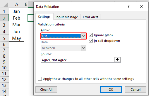
We can create a drop-down list in Excel using the “Data Validation in excelThe data validation in excel helps control the kind of input entered by a user in the worksheet.read more” tool, so as the word itself says, data will be validated even before the user decides to enter. So, all the values that need to be entered are pre-validated by creating a drop-down list in Excel. For example, assume we need to allow the user to choose only “Agree” and “Not Agree,” so we will create a list of values in the drop-down list.
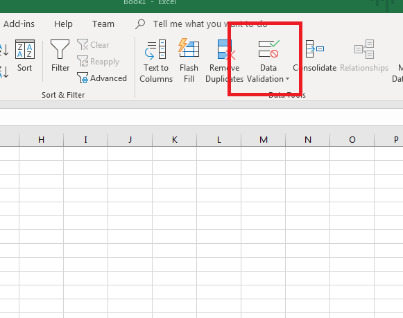
- In the Excel worksheet under the “Data” tab, we have an option called “Data Validation” from this again, choose “Data Validation.”

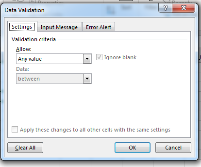
- As a result, this will open the “Data Validation” tool window.
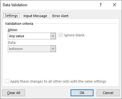
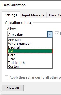
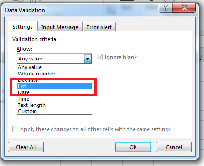
- The “Settings” tab will be shown by default, and now we need to create validation criteria. Since we are creating a list of values, choose “List” as the option from the “Allow” drop-down list.
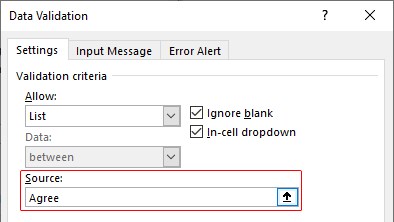
- For this “List,” we can give a list of values to be validated in the following way, i.e., by directly entering the values in the “Source” list.

- Enter the first value as “Agree.”
- Once the first value to be validated is entered, we need to enter “comma” (,) as the list separator before entering the next value. So, enter “comma” and enter the following values as “Not Agree.”
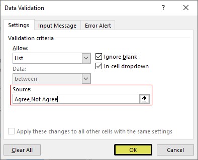
- After that, click on “Ok,” and the list of values may appear in the form of the “drop-down” list.

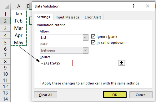
#2 – Create a List of Values from Cells
The above method is to get started, but imagine the scenario of creating a long list of values or your list of values changing now and then. Then, it may get difficult to return and edit the list of values manually. So, by entering values in the cell, we can easily create a list of values in Excel.
Follow the steps to create a list from cell values.
- We must first insert all the values in the cells.

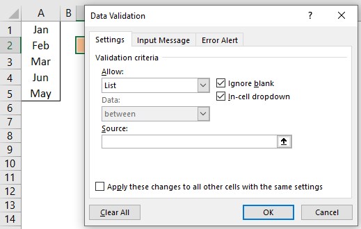
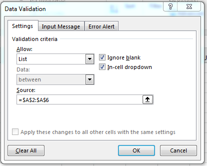
- Then, open “Data Validation” and choose the validation type as “List.”

- Next, in the “Source” box, we need to place the cursor and select the list of values from the range of cells A1 to A5.

- Click on “OK,” and we will have the list ready in cell C2.

So values to this list are supplied from the range of cells A1 to A5. Any changes in these referenced cells will also impact the drop-down list.
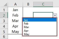
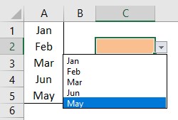
For example, in cell A4, we have a value as “Apr,” but now we will change that to “Jun” and see what happens in the drop-down list.
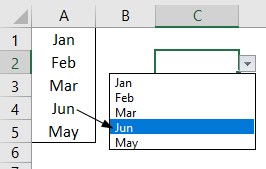
Now, look at the result of the drop-down list. Instead of “Apr,” we see “Jun” because we had given the list source as cell range, not manual entries.
#3 – Create List through Named Manager
There is another way to create a list of values, i.e., through named ranges in excelName range in Excel is a name given to a range for the future reference. To name a range, first select the range of data and then insert a table to the range, then put a name to the range from the name box on the left-hand side of the window.read more.
- We have values from A1 to A5 in the above example, naming this range “Months.”

- Now, select the cell where we need to create a list and open the drop-down list.
- Now place the cursor in the “Source” box and press the F3 key to an open list of named ranges.
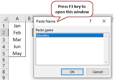
- As we can see above, we have a list of names, choose the name “Months” and click on “OK” to get the name to the “Source” box.
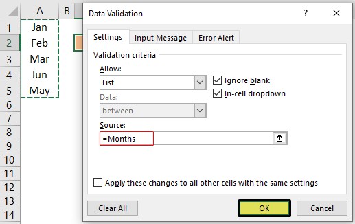
- Click on “OK,” and the drop-down list is ready.
Things to Remember
- The shortcut key to open data validation is “ALT + A + V + V.“
- We must always create a list of values in the cells so that it may impact the drop-down list if any change happens in the referenced cells.
Recommended Articles
This article has been a guide to Excel Create List. Here, we learn how to create a list of values in Excel also, create a simple drop-down method and make a list through name manager along with examples and downloadable Excel templates. You may learn more about Excel from the following articles: –
- Custom List in Excel
- Drop Down List in Excel
- Compare Two Lists in Excel
- How to Randomize List in Excel?
Excel for Microsoft 365 Excel 2021 Excel 2019 Excel 2016 Excel 2013 Excel 2010 Excel 2007 Excel Starter 2010 More…Less
When you want to display a list of values that users can choose from, add a list box to your worksheet.
Add a list box to a worksheet
-
Create a list of items that you want to displayed in your list box like in this picture.

-
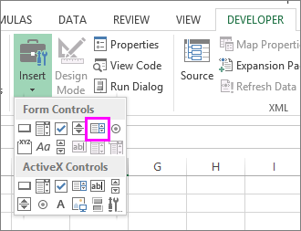
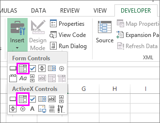
Click Developer > Insert.
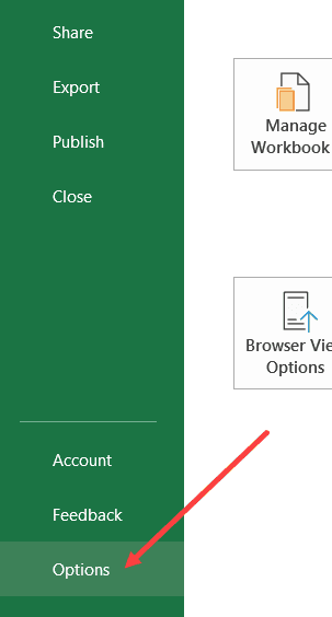
Note: If the Developer tab isn’t visible, click File > Options > Customize Ribbon. In the Main Tabs list, check the Developer box, and then click OK.
-
Under Form Controls, click List box (Form Control).
-
Click the cell where you want to create the list box.
-
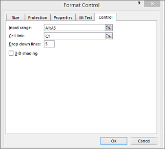
Click Properties > Control and set the required properties:
-
In the Input range box, type the range of cells containing the values list.
Note: If you want more items displayed in the list box, you can change the font size of text in the list.
-
In the Cell link box, type a cell reference.
Tip: The cell you choose will have a number associated with the item selected in your list box, and you can use that number in a formula to return the actual item from the input range.
-
Under Selection type, pick a Single and click OK.
Note: If you want to use Multi or Extend, consider using an ActiveX list box control.
-
Add a combo box to a worksheet
You can make data entry easier by letting users choose a value from a combo box. A combo box combines a text box with a list box to create a drop-down list.
You can add a Form Control or an ActiveX Control combo box. If you want to create a combo box that enables the user to edit the text in the text box, consider using the ActiveX Combo Box. The ActiveX Control combo box is more versatile because, you can change font properties to make the text easier to read on a zoomed worksheet and use programming to make it appear in cells that contain a data validation list.
-
Pick a column that you can hide on the worksheet and create a list by typing one value per cell.
Note: You can also create the list on another worksheet in the same workbook.
-
Click Developer > Insert.
Note: If the Developer tab isn’t visible, click File > Options > Customize Ribbon. In the Main Tabs list, check the Developer box, and then click OK.
-
Pick the type of combo box you want to add:
-
Under Form Controls, click Combo box (Form Control).
Or
-
Under ActiveX Controls, click Combo Box (ActiveX Control).
-
-
Click the cell where you want to add the combo box and drag to draw it.
Tips:
-
To resize the box, point to one of the resize handles, and drag the edge of the control until it reaches the height or width you want.
-
To move a combo box to another worksheet location, select the box and drag it to another location.
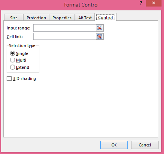
Format a Form Control combo box
-
Right-click the combo box and pick Format Control.
-
Click Control and set the following options:
-
Input range: Type the range of cells containing the list of items.
-
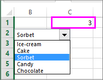
Cell link: The combo box can be linked to a cell where the item number is displayed when you select an item from the list. Type the cell number where you want the item number displayed.
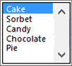
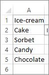
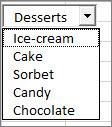
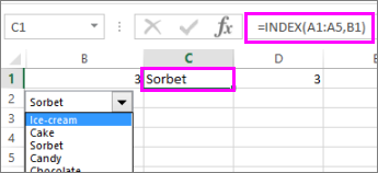
For example, cell C1 displays 3 when the item Sorbet is selected, because it’s the third item in our list.
Tip: You can use the INDEX function to show an item name instead of a number. In our example, the combo box is linked to cell B1 and the cell range for the list is A1:A2. If the following formula, is typed into cell C1: =INDEX(A1:A5,B1), when we select the item «Sorbet» is displayed in C1.
-
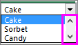
Drop-down lines: The number of lines you want displayed when the down arrow is clicked. For example, if your list has 10 items and you don’t want to scroll you can change the default number to 10. If you type a number that’s less than the number of items in your list, a scroll bar is displayed.
-
-
Click OK.
Format an ActiveX combo box
-
Click Developer > Design Mode.
-
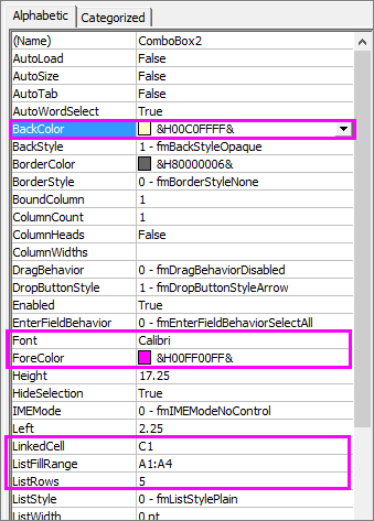
Right-click the combo box and pick Properties, click Alphabetic, and change any property setting that you want.
Here’s how to set properties for the combo box in this picture:
To set this property
Do this
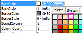
Fill color
Click BackColor > the down arrow > Pallet, and then pick a color.
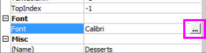
Font type, style or size
Click Font > the… button and pick font type, size, or style.
Font color
Click ForeColor > the down arrow > Pallet, and then pick a color.
Link a cell to display selected list value.
Click LinkedCell
Link Combo Box to a list
Click the box next to ListFillRange and type the cell range for the list.
Change the number of list items displayed
Click the ListRows box and type the number of items to be displayed.
-
Close the Property box and click Designer Mode.
-
After you complete the formatting, you can right-click the column that has the list and pick Hide.
Need more help?
You can always ask an expert in the Excel Tech Community or get support in the Answers community.
See Also
Overview of forms, Form controls, and ActiveX controls on a worksheet
Add a check box or option button (Form controls)
Need more help?
Want more options?
Explore subscription benefits, browse training courses, learn how to secure your device, and more.
Communities help you ask and answer questions, give feedback, and hear from experts with rich knowledge.
![]()
Download Article
![]()
Download Article
If you’re wondering how to create a multiple-line list in a single cell in Microsoft Excel, you’ve come to the right place. Whether you want a cell to contain a bulleted list with line breaks, a numbered list, or a drop-down list, inserting a list is easy once you know where to look. This wikiHow will teach you three helpful ways to insert any type of list to one cell in Excel.
-
1
Double-click the cell you want to edit. If you want to create a bullet or numerical list in a single cell with each item on its own line, start by double-clicking the cell into which you want to type the list.
-
2
Insert a bullet point (optional). If you want to preface each list item with a bullet rather than a number or other character, you can use a key shortcut to insert the bullet symbol. Here’s how:
- Mac: Press Option + 8.
-
Windows:
- If you have a numeric keypad on the side of your keyboard, hold down the Alt key while pressing 7 on the keypad.[1]
- If not, click the Insert menu, select Symbol, type 2022 into the «Character code» box at the bottom, and then click Insert.
- If 2022 didn’t bring up a bullet point, select the Wingdings font instead, and then enter 159 as the character code. You can then click Insert to add the bullet point.
- If you have a numeric keypad on the side of your keyboard, hold down the Alt key while pressing 7 on the keypad.[1]
Advertisement
-
3
Type your first list item. Don’t press Enter or Return after typing.
- If you want your list to be numbered, preface the first list item with 1. or 1).
-
4
Press Alt+↵ Enter (PC) or Control+⌥ Option+⏎ Return on a Mac. This adds a line break so you can start typing on the next line of the same cell.[2]
-
5
Type the remaining list items. To continue your list, just enter another bullet point on the second line, type the list item, and press Alt + Enter or Control + Option + Return to open a new line. When you’re finished, you can click anywhere else on your sheet to exit the cell.


Advertisement
-
1
Create your list in another app. If you’re trying to paste a bullet list (or other type of list) into a single cell rather than have it spread across multiple cells, there’s a trick to pasting the list. Start by creating your list in an app like Word, TextEdit, or Notepad.
- If you create a bulleted list in Word, the bullets will copy over to your cell when pasted into Excel. Bullets may not copy from other apps.
-
2
Copy the list. To do this, just highlight the list, right-click the highlighted area, and then select Copy.
-
3
Double-click a cell in Excel. Double-clicking the cell before pasting makes it so the list items will all appear in the same cell.
-
4
Right-click the cell. The context menu will expand.
-
5
Click the clipboard icon under «Paste Options.» The icon has a clipboard and a black rectangle. This pastes the list into the cell you double-clicked. Each list item will appear on its own line within the same cell.


Advertisement
-
1
Open the workbook in which you want to create a drop-down list. If you want to be able to click a cell to view and select from a drop-down list, you can create a list with Excel’s data validation tool.[3]
-
2
Create a new worksheet in the workbook. You can do this by clicking the + next to the existing workbook sheets at the bottom of Excel. This worksheet is where you’ll enter the items that you want to appear in your drop-down list.
- After you create the list on a separate sheet and add it to a table, you’ll be able to create a drop-down list containing the list data in any cell you want.
-
3
Type each list item into a single column. Enter every possible list choice into its own separate cell. The items you type will all be available in the drop-down list.
- If you plan to make a lot of drop-down menus and want to use this same sheet to create all of them, add a header to the top of the list. For example, if you’re making a list of cities, you could type City into the first cell. This header won’t actually appear on the drop-down list you create—it’s just for organization on this sheet that contains list data.
-
4
Highlight the entire table and press Ctrl+T. Include the header at the top of the list when highlighting. This opens the Create Table dialog.
-
5
Choose a header option and click OK. If you added a header to the top of your list, check the box next to «My table has headers.» If not, make sure there is no checkmark there before clicking OK.
- Now that your list is in a table, you can make changes to it after creating your drop-down list, and your drop-down list will update automatically.
-
6
Sort the list alphabetically. This will keep your list organized once you add it to your sheet. To do this, just click the arrow next to your header cell and select Sort A to Z.
-
7
Click the cell on the worksheet in which you want to add the list. This can be any cell on any worksheet in the workbook.
-
8
Type a name for the list into the cell. This is the cell where the list will appear, so give it a name that indicates the type of option you should choose from that list. For example, if you made a list of cities, you could type City here.
-
9
Click the Data tab and select Data Validation. Make sure the cell is selected before doing this. If you don’t see Data Validation in the toolbar, click the icon in the «Data Tools» section that has two black rectangles with a green checkmark and a red circle with a line through it. This opens the Data Validation window.
-
10
Click the «Allow» menu and select List. Additional options will expand.
-
11
Click the up-arrow in the «Source» field. This minimizes the Data Validation window so you can select your list data.
-
12
Select the list (without the header) and press ↵ Enter or ⏎ Return. Click back over to the tab that has your list data and drag the mouse cursor over just the list items. Pressing Enter or Return will add the range to the «Source» field.
-
13
Click OK. The selected cell now has a drop-down list. If you need to add or remove items from the list, you can simply make those changes on your new worksheet and they’ll automatically propagate to the list.


Advertisement
Ask a Question
200 characters left
Include your email address to get a message when this question is answered.
Submit
Advertisement
Thanks for submitting a tip for review!
About This Article
Article SummaryX
1. Double-click the cell.
2. Press Alt + 7 or Option + 8 to add a bullet point.
3. Type a list item.
4. Press Alt + Enter (PC) or Control + Option + Return (Mac) to go to the next line.
5. Repeat until your list is finished.
Did this summary help you?
Thanks to all authors for creating a page that has been read 62,222 times.
Is this article up to date?
Excel has some useful features that allow you to save time and be a lot more productive in your day-to-day work.
One such useful (and less-known) feature in the Custom Lists in Excel.
Now, before I get to how to create and use custom lists, let me first explain what’s so great about it.
Suppose you have to enter numbers the month names from Jan to Dec in a column. How would you do it? And no, doing it manually is not an option.
One of the fastest ways would be to have January in a cell, February in an adjacent cell and then use the fill handle to drag and let Excel automatically fill in the rest. Excel is smart enough to realize that you want to fill the next month in each cell in which you drag the fill handle.
Month names are quite generic and therefore it’s available by default in Excel.
But what if you have a list of department names (or employee names or product names), and you want to do the same. Instead of manually entering these or copy-paste these, you want these to appear magically when you use the fill handle (just like month names).
You can do that too…
… by using Custom Lists in Excel
In this tutorial, I will show you how to create your own custom lists in Excel and how to use these to save time.
How to Create Custom Lists in Excel
By default, Excel already has some pre-fed custom lists that you can use to save time.
For example, if you enter ‘Mon’ in one cell ‘Tue’ in an adjacent cell, you can use the fill handle to fill the rest of the days. In case you extend the selection, keep on dragging and it will repeat and give you the day’s name again.

Below are the custom lists that are already in-built in Excel. As you can see, these are mostly days and month names as these are fixed and will not change.

Now, suppose you want to create a list of departments that you often need in Excel, you can create a custom list for it. This way, the next time you need to get all the departments name in one place, you don’t need to rummage through old files. All you need to do is type the first two in the list and drag.

Below are the steps to create your own Custom List in Excel:
- Click the File tab

- Click on Options. This will open the ‘Excel Options‘ dialog box

- Click on the Advanced option in the left-pane

- In the General option, click on the ‘Edit Custom Lists’ button (you may have to scroll down to get to this option)

- In the Custom Lists dialog box, import the list by selecting the range of cells that have the list. Alternatively, you can also enter the name manually in the List Entries box (separated by comma or each name in a new line)

- Click on Add


As soon as you click on Add, you would notice that your list now becomes a part of the Custom Lists.

In case you have a large list that you want to add to Excel, you can also use the Import option in the dialog box.
Pro tip: You can also create a named range and use that named range to create the custom list. To do this, enter the name of the named range in the ‘Import list from cells’ field and click OK. The benefit of this is that you can change or expand the named range and it will automatically get adjusted as the custom list
Now that you have the list in Excel backend, you can use it just like you use numbers or month names with Autofill (as shown below).

While it’s great to be able to quickly get these custom lits names in Excel by doing a simple drag and drop, there is something even more awesome that you can do with custom lists (that’s what the next section is about).
Create Your Own Sorting Criteria Using Custom Lists
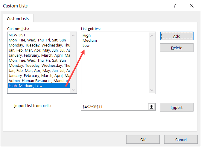
One great thing about custom lists is that you can use it to create your own sorting criteria. For example, suppose you have a dataset as shown below and you want to sort this based on High, Medium, and Low.

You can’t do this!
If you sort alphabetically, it would screw the alphabetical order (it will give you High, Low, and Medium and not High, Medium, and Low).
This is where Custom Lists really shine.
You can create your own list of items and then use these to sort the data. This way, you will get all the High values together at the top followed by the medium and low values.
The first step is to create a custom list (High, Medium, Low) using the steps shown in the previous section (‘How to Create Custom Lists in Excel‘).
Once you have the custom list created, you can use the below steps to sort based on it:
- Select the entire dataset (including the headers)
- Click the Data tab

- In the Sort and Filter group, click on the Sort icon. This will open the Sort dialog box

- In the Sort dialog box, make the following selections:
- Sort by Column: Priority
- Sort On: Cell Values
- Order: Custom Lists. When the dialog box opens, select the sorting criteria you want to use and then click on OK.

- Click OK


The above steps would instantly sort the data using the list you created and used as criteria while sorting (High, Medium, Low in this example).

Note that you don’t necessarily need to create the custom list first to use it in sorting. You can use the above steps and in Step 4 when the dialog box opens, you can create a list right there in that dialog box.
Some Examples Where you can Use Custom Lists
Below are some of the cases where creating and using custom lists can save you time:
- If you have a list that you need to enter manually (or copy-paste from some other source), you can create a custom list and use that instead. For example, this could be department names in your organization, or product names or regions/countries.
- If you’re a teacher, you can create a list of your student names. That way, when you are grading them the next time, you don’t need to worry about entering the student names manually or copy-pasting it from some other sheet. This also ensures that there are fewer chances of errors.
- When you need to sort data based on criteria that are not in-built in Excel. As covered in the previous section, you can use your own sorting criteria by making a custom list in Excel.
So this is all that you need to know about Creating Custom Lists in Excel.
I hope you found this useful.
You may also like the following Excel tutorials:
- How to Sort by the Last Name in Excel
- How to SORT in Excel (by Rows, Columns, Colors, Dates, & Numbers)
- How to Sort By Color in Excel
- How to Sort Worksheets in Excel
- Automatically Sort Data in Alphabetical Order using Formula
A Custom List in Excel is very handy to fill a range of cells with your own personal list.
It could be a list of your team members at work, countries, regions, phone numbers, or customers. The main goal of a custom list is to remove repetitive work and manual errors.
It is extremely useful when you need to fill in the same data from time to time. There are two options to create a list in Excel that can be used repeatedly by using the fill handle.
In this tutorial, you will learn how to create a list in Excel:
- Using Pre-existing List
- Create a list in Excel manually
- Import from another worksheet
Let’s look at each of these methods one-by-one!
Watch it on YouTube and give it a thumbs-up!

Download this Excel Workbook and follow along with the tutorial on how to create a list in Excel :
Using Pre-existing List
At first, it might seem like magic how Excel does this!
There are some lists that are already stored in Excel like days of the week and months in a year.

To demonstrate the power of Excel’s Custom Lists, we’ll explore what’s currently in Excel’s memory as a default list:
STEP 1: Type February in the first cell

STEP 2: From that first cell, click the lower right corner and drag it to the next 5 cells to the right

STEP 3: Release and you will see it get auto-populated to July (The succeeding months after February)

Create a list in Excel manually
You can also manually add new values in the Custom List box and re-use them whenever you wish to.
Let us go straight into the Options in Excel to view how it’s being done, and how you can create your own Custom List:
STEP 1: Select the File tab

STEP 2: Click Options

STEP 3: Select the Advanced option

STEP 4: Scroll all the way down and under the General section, click Edit Custom Lists.

Here you can see the built-in default Excel lists of the calendar months and the days.
If you click on a Custom List, you will see under List entries that it is greyed out and you cannot make any changes. This indicated that it is a default Excel Custom List.

STEP 5: You can create & add your own Custom List under the List entries section.
Click on NEW LIST under the Custom Lists area and then manually enter your list, entering one entry per line:

After typing the values, click Add.
In our screenshot below, we added the values of the Greek alphabet (alpha, beta, gamma, and so on)
Click OK once done.

STEP 6: Click OK again

STEP 7: Now let’s go back into our Excel workbook to see our new Custom List in action. Type alpha on a cell.

STEP 8: From that cell, click the lower right corner and drag it to the next 5 cells to the right

STEP 9: Release and you will see it get auto-populated to zeta, which is based on our Custom List created in Step 8

Next up is a demonstration of how to make a list in Excel by importing data from another worksheet.
Import from another worksheet
You can easily import a custom list from another worksheet. Follow the steps below to get this done:
STEP 1: Go to the File Tab.

STEP 2: Select Options from the left panel.

STEP 3: In the Excel Options dialog box, select Advanced.

STEP 4: Under the General section, click on the Edit Custom List button.

STEP 5: In the Custom List dialog box, select the small arrow up button.

STEP 6: Select the range containing the custom list.

STEP 7: Click on Import.

STEP 8: Once the list will appear under list entries and click OK.

STEP 9: Click OK.

Now, your custom list is stored in Excel!
STEP 10: Type the first entry of the list “XS” in cell A8.

STEP 11: From that first cell, click the lower right corner and drag it to the next 6 cells to the right.

The entire list will be displayed in the selected range!

You can even create this list vertically. Simply, type the XS in a cell. Click on the lower right corner and drag the cell downwards.

The list will appear vertically!
Conclusion
In this article, you have learned how to make a list in Excel so that you don’t have to type the same list over and over again. You use the Custom list feature in Excel and store it in Excel and use it whenever necessary.
You can either use the pre-existing list, manually type the list or link it from another worksheet!
Make sure to download our FREE PDF on the 333 Excel keyboard Shortcuts here:

You can learn more about how to use Excel by viewing our FREE Excel webinar training on Formulas, Pivot Tables, Power Query, and Macros & VBA!

Bottom Line: Learn 4 different techniques for creating a list of numbers in Excel. These include both static and dynamic lists that change when items are added or deleted from the list.
Skill Level: Beginner
Watch the Tutorial
Download the Excel File
You can download the worksheet that I use in the video here:
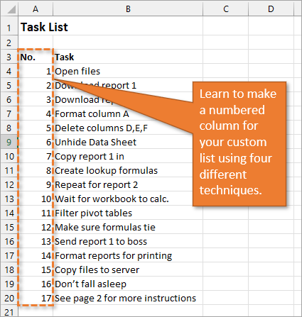
If you have a list of items in Excel and you’d like to insert a column that numbers the items, there are several ways to accomplish this. Let’s look at four of those ways.
1. Create a Static List Using Auto-Fill
The first way to number a list is really easy. Start by filling in the first two numbers of your list, select those two numbers, and then hover over the bottom right corner of your selection until your cursor turns into a plus symbol. This is the fill handle.
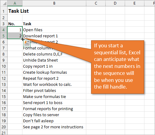
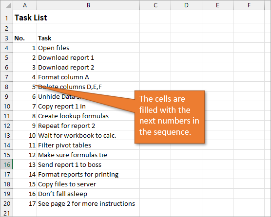
When you double-click on that fill handle (or drag it down to the end of your list), Excel will fill in the blanks with the next numbers in the sequence.
An alternate way to create this same numbered list is to type a 1 in the first cell and then double-click the fill handle. Because Excel doesn’t have a second number to identify a sequence or pattern, it will fill down the columns with 1s. But you will notice that a menu is available at the end of your column, and from that menu, you can select the option to Fill Series. This will change the 1s to a sequential list of numbers.
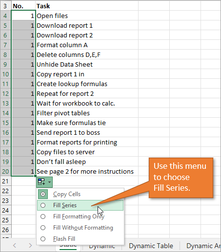
The numbered column we’ve created in both instances is static. This means it doesn’t change when you make additions or deletions to the corresponding list of items. For example, if I insert a new row in order to add another task, there is a break in the numbered column as well, and I would have to repeat the same steps to correct the list.
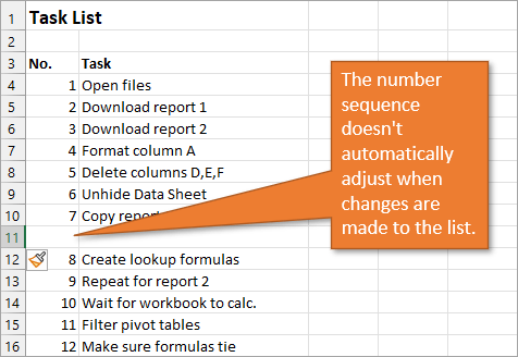
So, unless we want the numbers to always remain as they are, a better option would be to create a dynamic list.
2. Create a Dynamic List Using a Formula
We can use formulas to create a dynamic list where the numbers update when we add or delete rows from the list.
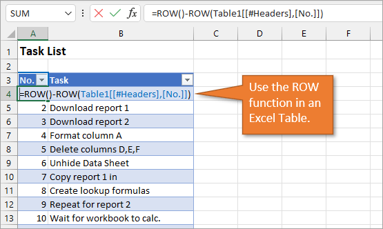
To use a formula for creating a dynamic number list, we can use the ROW function. The ROW function returns the row number of a cell. If we don’t specify a cell for ROW, it just returns the current row number of whatever is selected.
In our example, the first cell in our list doesn’t start on Row 1. It starts on Row 4. But we don’t want our list to start at 4; we want it to start at 1. To subtract the extra 3, our formula will include a minus sign and then the ROW function again, but this time pointed to the cell above our formula (which is in Row 3).
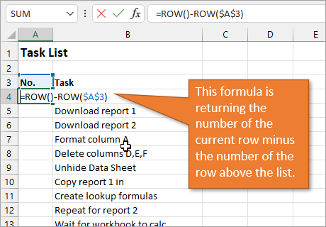
We use the absolute values (dollar signs) in our cell selection because we don’t want that number to change as we copy the formula down the list. In other words, we always want to subtract 3 from the row number to give us our list number.
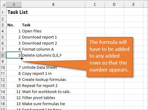
When we copy down the formula, we have a numbered list that will adjust when we add or delete rows. However, when adding a row, we will have to copy the formula into the newly inserted cell.
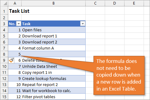
This additional step of copying the formula into new rows can be avoided if we use Excel Tables.
3. Create a Dynamic List Using a Formula in an Excel Table
If we write the same formula but we use an Excel table, the only difference we will make in the formula is that we reference the column header instead of the absolute cell value.
Because we are using an Excel Table, the formula automatically fills down to the other rows. When we add a row to the table, the formula will automatically populate in the new cell.
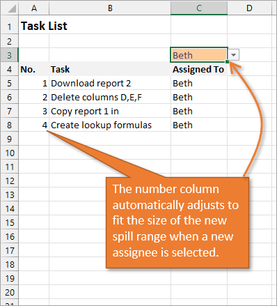
4. Create a Dynamic List Using Dynamic Array Formulas
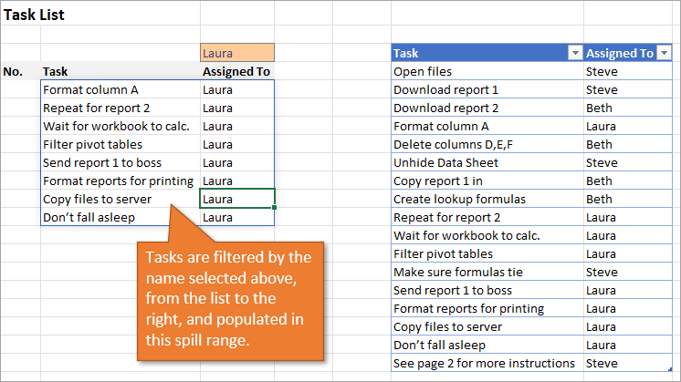
Below, I have a table that is populated using Dynamic Array Formulas. The FILTER formula spills a range of results based on whatever name is selected in the orange cell.
The Dynamic Array formula we will use is SEQUENCE. This will return a sequence for the number of rows we identify in the formula. To tell Excel how many rows there are, we will use the ROW function as the argument for sequence. The argument for ROW is just the spill range. The way to notate the spill range is to simply place a hashtag after the name of the first cell in the range. So our formula looks like this:
=SEQUENCE(ROWS(B5#))
Once we complete our formula and hit Enter, the list will be numbered.
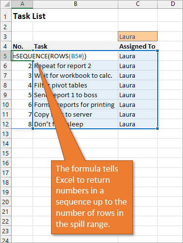
With this formula in place, if the size of the range changes when a new name is selected, the numbered column for the list will automatically adjust as well.
Bonus Tip: Formatting Your Numbered List
If you want to add periods or other punctuation to your numbered list:
- Select the entire list and right-click to choose Format Cells. Or use the keyboard shortcut Ctrl + 1.
- Choose the Custom option on the Number tab.
- Then in the Type field, type in the number 0 with whatever punctuation you would like to surround your number.
Here, I’ve just added a period.
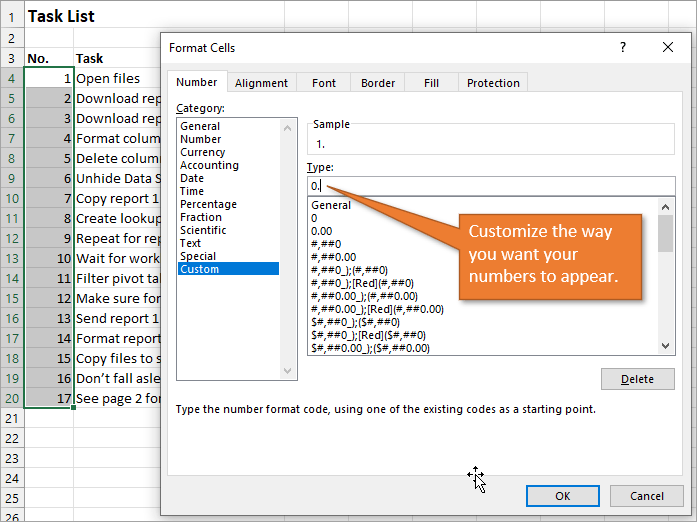
When you hit OK, you will have formatted the entire selection.
Related Posts
Here are a few similar posts that may interest you.
- Excel Tables Tutorial Video – Beginners Guide for Windows & Mac
- New Excel Features: Dynamic Array Formulas & Spill Ranges
- How to Prevent Excel from Freezing or Taking A Long Time when Deleting Rows
Conclusion
I hope these four ways to create ordered lists are helpful for you. If you have questions or feedback, I would love to hear them in the comments. Have a great week!

Excel 2019 is used in many organizations to fill out information on customers, orders and products. Some of the data items are repetitive, meaning that you don’t type data into a cell but rather select from a data list. For instance, you might want to select a state from a dropdown list in a column that stores the state for a customer address. You can make it easier to fill out forms in Excel 2019 using data lists, and this article shows you how to create them.
Set Up the List
Before you create a dropdown list in Excel, you need a list of data to use. Since you can make multiple worksheets in one Excel workbook, most people use a separate sheet to populate the data list. You can then configure any specific cell in the Excel form to point to this list of data. You then set the cell as a list, and Excel does the rest for you.
You don’t have to use a separate sheet to populate a data list. You can use the same sheet or even a separate workbook. You can use a separate workbook, but any changes to this workbook could affect the data list. Also, if the workbook is moved to a different directory or storage location, your list will no longer function.
For simplicity, this article’s examples use the same workbook and worksheet, but just know that you can use references to separate worksheets and workbooks for your own data lists.
Create a blank worksheet in a currently opened workbook, or you can create a new workbook to store the new data list. In the following scenario, a list of states is used for a data list. We’ll add five states to the first column (A) in a new worksheet.
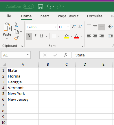
(List of states set up for a dropdown)
In the image above, five states were added to their own cells. Notice at the top that «State» is used to label the column list. This is beneficial for the dropdown that we’ll make, and it helps label data so that others can understand what the list is used for. The list can be as long as it needs to be, but we’ve only added five states for simplicity.
You now need a place to display the dropdown that will contain these values. For simplicity, we’ll set up a dropdown in the same worksheet. Make sure that you label the dropdown as well so that users know what the dropdown list is for.
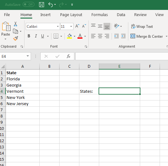
(Location of the state dropdown and its label)
In the image above, the cell E4 is selected as the cell that will contain the dropdown list. In D4, the label «States:» is displayed so that users know a list of states will be shown in the dropdown. It also helps users understand that they must select a state when they fill out the form. Labeling cells is an important part of creating effective spreadsheets that store the right data, especially among several users that add data and revise it periodically.
Creating a Dropdown Based on External Data
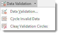
With the cell next to the «States:» label selected, click the «Data» tab. The «Data» tab has several data tools that you can use to work with lists. Click the «Data Validation» button, which is found in the «Data Tools» section of the «Data» tab.
(Location of the «Data Validation» button)
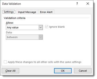
Clicking this button displays another dropdown selection. Click the «Data Validation» option, and a new window opens where you can configure your data list and cell that contains the options for a user to choose from.
(Data validation configuration window)
In the window above, you have several options to set a dropdown using a list of data. For a dropdown, you need to choose the «List» option. The «List» option is found in the «Allow» dropdown box.
(Select «List» for the validation criteria)
In the image above, notice that the «Allow» dropdown has the «List» option selected. This option tells Excel 2019 that you want to use a data list. If you hadn’t already created a data list in an external workbook or in a worksheet in the current workbook, you would need to cancel out of this window and create a list. For this reason, it’s better to create a list of data that you want to display in a dropdown before setting up this configuration option.
When you select «List» from the dropdown, a new list of options display in the «Data Validation» window. The «Source» text box is where you can type the range of cells. With a list of only five states, it’s easy to take a look at the cells that contain states and type them into this text box. However, when you have a range of cells that span several rows, you’d have to scroll down the spreadsheet to find the last cell in the list. You could also have empty cells that you miss as you scroll down the list. Instead of typing the cell range manually, you can click the arrow up button adjacent to the «Source:» text box. This opens a view of your spreadsheet where you can use your mouse to select the cells that contain a list of data.
Click the arrow button next to the «Source» text box to trigger the data selection feature. The «Data Validation» window collapses and then only the Source text box displays. Use the mouse to highlight each state. You don’t need to click the states individually. Instead, click the first state and drag your mouse to the last state in the list. The data validation tool will automatically create the range in the text box with the right textual labels that reference cells containing the information to display in the dropdown.
(Data list selected and displayed in Source text box)
Click the «Input Message» tab to see a list of options to prompt the user with information when the input cell is selected. In some scenarios, having a label such as «State» is not enough to explain what the user should input. You might need additional information to explain what is needed using a prompt. You could set a Note but these notes are used for revisions and not the best option for setting instructional information. With an Input Message, you can prompt the user and display additional information when the cell is selected.
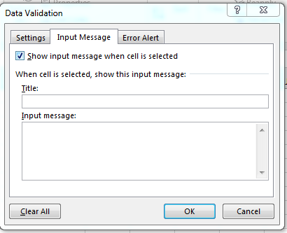
(Input message configuration window)
The input configuration window contains a title and an input message. The «Title» text box is where you set up the main title that the user will see when clicking the cell. The «Input Message» is arguably the more important input text box. This text box describes the purpose of the input selected by the user. It gives additional information to help the user understand the right data selection when filling out the Excel 2019 form.
Fill out these two input fields if you think more information is needed for the user as the form is filled out. Click the «Error Alert» tab to set up an error message or warning for the user should one occur.
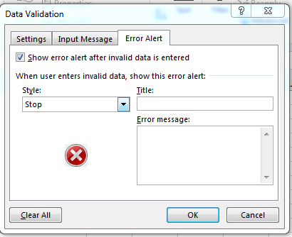
(Error alert option for a data dropdown)
In the configuration window above, the check box labeled «Show error alert after invalid data is entered» tells Excel to stop the user and display the configured error should the user enter invalid input. For instance, we have five states from which the user can select in a dropdown. If the user decides to enter a state that isn’t in the list, then Excel would display an error and prompt the user to re-enter information to valid input. You can remove this selection to skip the option, but you should only skip this option if you do not want to restrict data entry to only what’s available in the dropdown list.
In the «Style» dropdown, you can choose if you want to stop the user (the default), or if you want the message to show as an informational note or a warning. This gives you granular control of invalid data errors, so that you can choose if you want to allow the user to continue filling out the form even if data is incorrectly entered.
The «Title» and «Error message» input boxes are the text displayed to the user. Just like the ‘Input Message» option, the «Error message» text box is the most important because it gives the user detailed information on why the input is invalid.
After you make your choices in all three tabs, click the «OK» button, and Excel 2019 sets up the dropdown list in the selected cell.
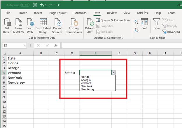
(Dropdown using a data list)
You can test the new dropdown data list by selecting data. You can also test the error messages by setting the cell to a state that does not match one in the set list.
For instance, first click the arrow in the dropdown and select «Florida.» Notice that no error message is displayed. Next, click the dropdown cell, which is E4 in this example. Type the word «Text» in the input cell. Click away from the input cell by clicking cell F1. Notice that an error message displays indicating that incorrect input was detected.
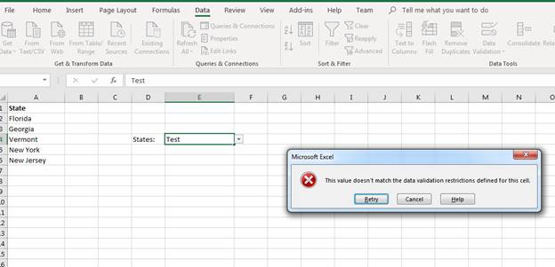
(Error message displayed from invalid input)
This error and validation control let you stop invalid input so that you can keep a spreadsheet of data that follows a strict rule set. By blocking invalid input, you can ensure that only a specific set of data is added to your input forms.
Dropdown lists are a common part of forms, and Excel makes it easy to create them whether the list contains 2 or 2000 cells. Dropdown lists are valuable when you have a set list of items from which you want users to choose, so they cannot just type any value into a cell. Using data lists makes creating long forms with multiple dropdown lists faster and remember that you aren’t limited to just the current sheet. You can reference any worksheet or workbook that contains your data by just adding the appropriate reference syntax in your data validation options.
Managing Data
Entering and managing lots of data can be a daunting task. It’s easy to get overwhelmed in all of those rows and columns of information. The solution is to use a form. A form is simply a dialog box that lets you display or enter information one record (or row) at a time. It can also make the information more visually appealing and easier to understand.
Most people who are familiar with the MS Office suite associate complex forms with Excel’s sister program Access, but you can use them in Excel as well. In fact, you can even share data between the two programs.
There are two kinds of forms available in MS Excel: data forms and worksheet forms.
-
Data forms are generally used for data entry. They are simple forms that list the contents of a single column. What’s more, they can display up to 32 fields at a time. This is especially helpful when dealing with a data range that reaches across more columns than will fit on a screen. You can insert, alter, delete, and even find records with data forms.
-
Worksheet forms are more sophisticated and specialized. They can be customized to fit the information at hand or to fill a particular need. They can even be complex and appealing enough to be printed or distributed online. Worksheet forms must be created using the Microsoft Visual Basic Editor.
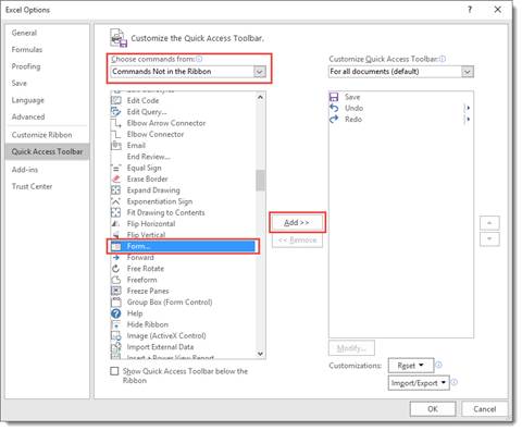
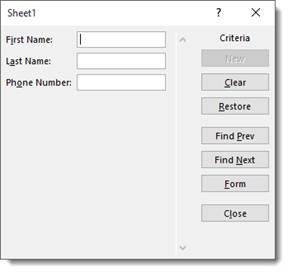
Adding the Form Button to the Quick Access Toolbar
The Form button is not included in the ribbon, but you can add it to the Quick Access Toolbar, which, if you remember, is in the upper left hand corner of the application window.
To add the Form button, click the arrow to the right of the Quick Launch toolbar and select More Commands. This will launch the Excel Options window, which can also be accessed by clicking Options on the File tab.
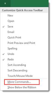
In the «Choose commands from» box, select Commands Not In the Ribbon, then scroll down through the list until you find Forms. Select it and click Add. When you are finished, click OK.
This is what the Form button looks like:  .
.
Adding Records Using the Data Form
When you click the Form button for the first time, Excel will analyze the row of field names and entries for the first record. It uses that information to create a data form.
Let’s click on the Form button now.
The first record appears in the dialogue box:
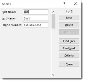
Click Find Next to find the next record.
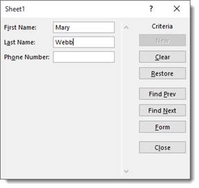
If you want to add a new record using the data form, click New.
As you can see in the snapshots above, the number of the record appears above the New button.
However, when you click the New button, it lets you know that it’s a new record.
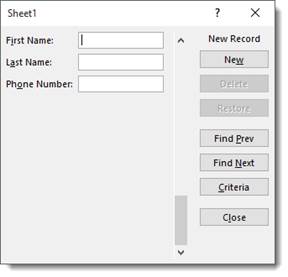
Let’s add a new record.
Enter the information, then hit Enter.
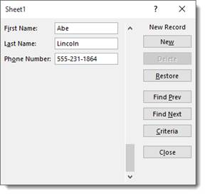
The new record appears in your list:
You can hit ESC when you’re done adding records.
Editing Records in the Data Form
In addition to adding records, you can also edit them. You can use the data form to find records that need updated or removed from the list.
To do this, click the Form button on the Quick Access Toolbar.
Find the record that you want to update or remove.

Now click in any of the fields to update the data. You can also delete data in the field.
Hit Enter.
Navigating Through Records in the Data Form
If you have a lot of records, navigating through them can be a challenge. The data form makes it a bit easier.
If you want to move to the next record in the data form, press Enter or the down arrow key.
To move to the previous record, hit the up arrow or press Shift+Enter.
To move to the first record in the data list, press CTRL+ ? (up arrow) or press CTRL+PgUp.
To go to a new data form that comes after the last record, press CTRL+ ? (down arrow) or CTRL+PgDn.
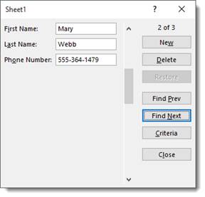
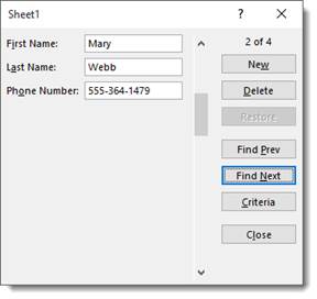
Find Records in the Data Form
If you want to find a specific record, you can use the Criteria button in the data form. It’s pictured below.
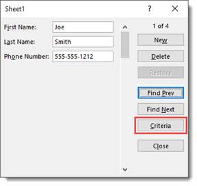
When you click the Criteria button, Excel 2019 clears the field entries in the data form. Instead, the word Criteria is displayed.
Let’s push the Criteria button to show you what we mean.
We now see a blank data form.
Notice that the word Criteria is above the new button, and the new button is inactive since we’re searching for a record.
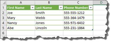
Now, let’s say you’re looking for a woman named Mary Webb, but you have 5000 women named Mary in your list.
Enter the criteria: Mary Webb.
Now click the Find Next button.
As you can see, it brings up the record.
You can also include the following operators in search criteria to help you find the record you need:
-
? for single
-
* for multiple wildcard characters
-
= Equal to
-
> Greater than
-
< Less than
-
>= Greater than or equal to
-
<= Less than or equal to
-
<> Not equal to
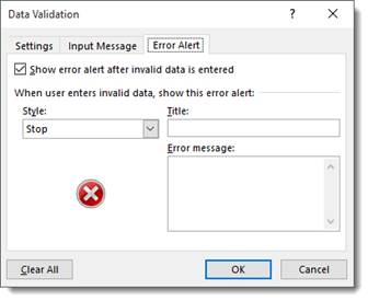
Data Validation
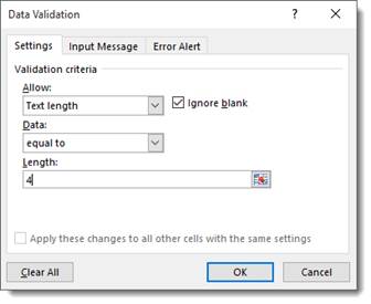
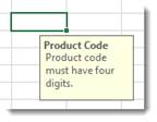
Data Validation lets you choose what information is acceptable to enter into a cell. For instance, you may have a product code that has four digits. You can set up a cell so that anything other than a 4-digit number will display an error message.
To set up data validation, select a cell or cells, then click the Data tab. Go to Data Validation in the Data Tools group.
Choose Data Validation from the dropdown menu.
You’ll see this window:
Since we’re going to set up a cell to accept only a 4-digit number, we will select Text length from the drop down menu that says «Allow» over it. From the Data dropdown menu, we are going to select «equal to» and in the length text field we will type «4.» That tells Excel we want an entry with four characters.
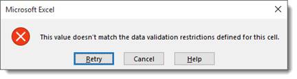
From here, we can hit OK and have Excel 2019 provide a generic warning that looks like this:
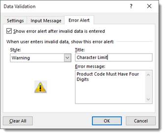
Alternatively, we can create a custom warning by selecting the Error Alert tab. Which looks like this:
Here we have selected the Warning style and entered the text for our error alert.
When a user enters a code of less or greater than four digits, the message will look like this:
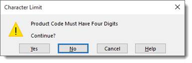
There are three kinds of error messages available in Excel: information messages, warning messages, and stop messages. Information messages and warning messages do not prevent invalid information to be entered into the cell; they simply inform the user that such an entry has been made. Users can choose to ignore the warning. A stop message, on the other hand, will not allow an invalid entry. It has two buttons, Cancel and Retry. Cancel restores the cell to its original value, and retry returns them to the cell for further editing.
You can also set up a message to remind users what the restrictions or expectations are. Use the Input Message tab to create a custom reminder.
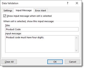
It will display anytime the cell or the range of cells is selected, as in the example below.
Auditing
MS Excel gives you a variety of tools to audit information in a worksheet. Just like data forms, formula auditing can take some of the confusion and frustration out of dealing with lots of different formulas. You can also see which cells have invalid information in them.
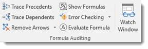
To use these tools, go to the Formulas tab, then the Formula Auditing group.
Select Error Checking and choose Error Checking from the dropdown menu.
That said, it is not always apparent which cells have formulas in them. Therefore, the first step to evaluate the formulas is to find them. Click the Show Formulas button, as highlighted below.
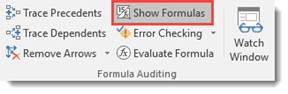
As you can see in the example below, the whole numbers will be changed to the formulas and the formula cells will be selected.
To make it easier to see the cells when they are no longer selected, you can click the fill  button. This will fill the selected cells with very visible yellow.
Let’s take a closer look at the other functions in the Formula Auditing group.
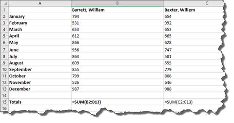
These two buttons allow you to trace (and turn off trace) precedents in a formula. A precedent cell is one that is referred to by a formula in another cell.
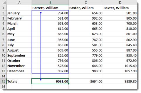
B2 thru B13 are precedents because they are referred to in the formula in cell B15. As you can see, the trace precedents button shows you the relationship between the cells.
The next button removes all arrows. 
The Watch Window (pictured below) is useful when you’re not sure if alterations to the value in a cell will affect a formula. You can easily remind yourself of the formula by adding it to the watch window.

The Evaluate Formula function will perform the calculations of a formula in slow motion so you can see each step. To use it, select a formula, then click the Evaluate Formula button  in the toolbar. You will see a box that looks like this:
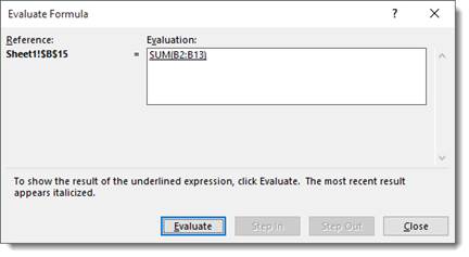
Click the Evaluate button to see Excel 2019 perform the calculations in slow motion. Use the Step In and Step Out buttons to navigate through each step in the formula.
Introduction to Data Plotting Using 3D Maps
Excel lets you explore your data in a worksheet by plotting it on a map. For example, you might want to create a 3D map to show the cities where your customers live. You will need an image of a map in either .jpg, .png, or .bmp format. If the data you wish to plot on a map doesn’t relate to cities, but perhaps instead locations in a warehouse, you’ll want to upload an image that relates to your data. That said, you will also need data that relates to the picture so that your data can be plotted using an XY coordinate system.
To create the 3D map, go to the Insert tab, then click the 3D Map button.

It may take a moment to load, but you will see the 3D Map screen.
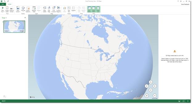
To create a map customized for your data, click New Tour.

Go to Home>New Scene in the 3D Map screen.
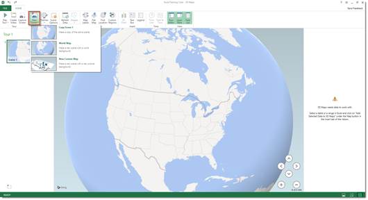
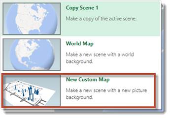
From the dropdown menu, select New Custom Map.
You will then see this dialogue box:
Locate the background picture you want to use.
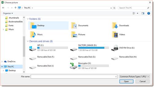
Click Open.

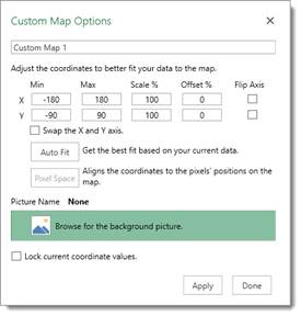
You can now see your picture open in the 3D Map window. Use the dialogue box to adjust the XY coordinates if needed.
Click Apply, then Done.
![]()
Creating a list in Excel
A list is a sequence of rows of related data. You can use lists whenever you need to organize large amounts of similar data, such as a database of names and addresses. You create a list in much the same way you create a worksheet. You enter information into a list by entering data into cells. Although you can change list elements after you have created a list, it is best to spend time planning your list before you begin entering data.
You plan your list by determining the column labels you want to include, the type of desired output, and how you might want to report or sort information in your database. For example, if you need to sort the list by last name, be sure to include a separate field for last names.
Identifying the Parts of a List
A list consists of records and fields. A record is a set of related data that corresponds to a row in the list. It contains alphanumeric data that, for example, might refer to the name, address, zip code, and telephone number of one person. Records are organized into fields according to the columns in your list and named according to the column labels. For example, you might name a field Last Name, Address 2, or Phone Number. The parts of a list are shown in Figure 1-1.
Each column of information in a list must have a column label as Excel uses these column labels as field names. You must start your first row of data directly below the column labels. If you don’t, Excel won’t recognize the column labels as belonging to the list. If you need to differentiate the column labels from the data, underline the labels or use a border along the bottom of the row of column labels.
For instructor-led MS Excel classes in Los Angeles call us on 888.815.0604.
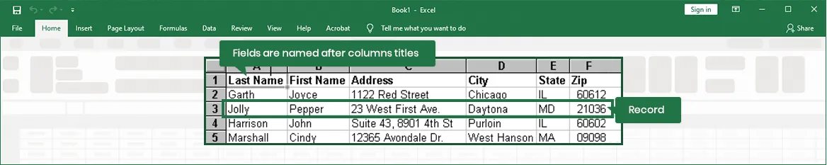
Figure 1-1: Parts of a List
Entering Column Labels in a List
Once you have decided which fields you need and how you would like them displayed in your list, you can enter the column labels. You enter column labels into the worksheet the same way you would enter text into a worksheet cell.
Remember the following rules when creating column labels:
- Use only alphanumeric characters.
- Column labels must be in the row directly above the data.
- Column labels can be up to 32,767 characters long, but shorter names are easier to use.
- Column labels must be unique.
- Don’t put blank rows or dashed lines under the column labels.
- Don’t use labels that look like range names, formulas, or cell addresses.
Method
To enter column labels in a list:
- In the first cell of the first row of the list, enter a column label.
- Move one cell to the right.
- Enter the second column label.
- Repeat steps 2 and 3 until finished.
Exercise
In the following exercise, you will enter column labels in a list.
- Start Excel. [Excel loads, and Book 1 opens. Sheet 1 is the active sheet].
-
In Sheet 1, in cell A2:H2, type the column labels listed below, in order, formatting the cells in Arial, 12 points, bold
ID NO
MAKE
MODEL
DOORS
AUTO
CONVRT
IN
RATE - If necessary, adjust the column widths of the worksheet so that you can clearly see all the field names.
- Save the workbook as Auto Research.
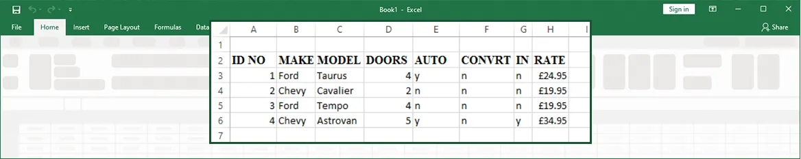
Figure 1-2: List Data
In this article, we will show you how to create, delete, and use a Custom List in Microsoft Excel. The Custom List feature is useful for the users who have to type a specific list in every Excel spreadsheet. If this is the case with you, this post will help you save time.

How can an Excel Custom List make your work easier and faster?
Excel has some built-in Lists that include names of the days and names of the months. You cannot edit or delete these built-in lists. Let’s understand the benefits of these built-in lists. Let’s say, you have to prepare data for weekly analysis of rainfall. In this data, you have to enter days’ names. If you do not know the usage of the Custom Lists, you have to type the days’ names manually which will take time. On the other hand, the user who knows the usage of the Custom List will type only the name of the day, say, Monday, and drag the cell. After that, Excel will fill all the cells with the days’ names in the correct order. This is how a Custom List makes your work easier and faster.
Can you create your own Custom List in Excel?
Yes, you can create your own Custom List in Excel. You can find the respective option int he Advanced category. From here, you need to use the Edit Custom Lists option to start creating the list. In this article, we have explained the process of creating, deleting, and using a Custom List in Microsoft Excel.
The steps to create a Custom List in Microsoft Excel are as follows:
- Launch Microsoft Excel and create a Custom List.
- Go to “File > Options.”
- Select the Advanced category from the left pane.
- Click on the Edit Custom Lists button.
- Import your Custom List from the Excel worksheet.
- Click OK.
Let’s see these steps in detail.
1] Launch Microsoft Excel and create a Custom List. Here, we have created a sample list of names of some states of the USA.
2] Click on the File menu and then select Options. This will open the Excel Options window.
3] In the Excel Options window, select the Advanced category from the left side. Now, scroll down the right side and click on the Edit Custom Lists button. You will find this button in the General section.

4] Now, click inside the box next to the Import list from cells. After that, select the range of the cells to insert the list. See the below screenshot.

5] Click on the Import button. When you click on the Import button, your list will be added to the Custom LIsts menu. Now, click OK and exit the Excel Options window.
You can also create a Custom List from the List Entries box. For this, first, type your Custom List in the List entries box and then click on the Add button. This will add your list to the Custom Lists menu.

How do I delete a Custom List in Excel?
Deleting a Custom List is easy. You need to select the list that you want to delete and then click on the Delete button. We have explained the steps for the same above in this article. No matter whether you have one or multiple lists in your spreadsheet, you need to follow the same steps to delete them all.
We have learned how to create a Custom List in Excel. Now, let’s see how to delete a Custom List in Excel. As we have described previously in this article, you cannot delete the built-in list in Excel. But you can delete those you have created.

To delete a Custom List in Excel, go to “File > Options > Advanced > Edit Custom Lists.” After that, select the list that you want to delete from the Custom Lists menu and then click on the Delete button. A popup window will appear showing you a message “List will be permanently deleted.” Click OK. This will delete the Custom List from Excel.
How to use a Custom List in Excel
Now, let’s talk about how to use a Custom List in Excel.

Follow the instructions below:
- Click on a cell in the document in which you want to insert your Custom List.
- Type the name from which your Custom List starts.
- Drag the cells to the bottom. This will fill up all the remaining entries automatically.
What are the two ways to create a Custom List?
The following are the two ways to create a Custom List in Microsoft Excel:
- By using the Import option.
- By using the List Entries box.
We have explained both of these methods above in this article.
That’s it.
Read next:
- How to create a Combination Chart in Microsoft Excel.
- How to create a drop-down list in Excel and Google Sheets.
If you create a custom list in Excel, you can easily fill a range with your own list of departments, clients, cities, credit card numbers, etc. This can save time and reduce errors.
First, we will look at an example of a built-in list.
1. Type Sun into cell B2.

2. Select cell B2, click on the lower right corner of cell B2 and drag it across to cell H2.

How does Excel know this?
3. On the File tab, click Options.
4. Under Advanced, go to General and click Edit Custom Lists.

Here you can find the built-in ‘days of the week’ lists. Also notice the ‘months of the year’ lists.
5. To create your own custom list, type some list entries, and click Add.

Note: you can also import a list from a worksheet.
6. Click OK.
7. Type London into cell C2.

8. Select cell C2, click on the lower right corner of cell C2 and drag it down to cell C5.

Note: a custom list is added to your computer’s registry, so you can use it in other workbooks.