Create database with excel

Do you need to create and use a database? This post is going to show you how to make a database in Microsoft Excel.

Excel is the most common data tool used in businesses and personal productivity across the world.

Since Excel is so widely used and available, it tends to get used frequently to store and manage data as a makeshift database. This is especially true with small businesses since there is no budget or expertise available for more suitable tools.

This post will show you what a database is and the best practices you should follow if you’re going to try and use Excel as a database.

Get the example files used in this post with the above link and follow along below!

What is a Database?

A database is a structured set of data that is often in an electronic format and is used to organize, store. and retrieve data.

For example, a database might be used to store customer names, addresses, orders, and product information.

Databases often have key features that make them an ideal place to store your data.

Database vs Excel

An Excel spreadsheet is not a database, but it does have a lot of great and easy-to-use features for working with data.

Here are some of the key features of a database and how they compare to an Excel file.

Feature	Database	Excel
Create, read, update, and delete records	✔️	✔️ Excel allows anyone to add or edit data. This can be viewed as a negative consideration.
Data types	✔️	⚠️ Excel allows for simple data types such as text, numbers, dates, boolean, images, and error values. But lacks more complex data types such as date and timezones, files, or JSON.
Data validation	✔️	⚠️ Excel has some data validation features, but you can only apply one rule at a time and these can easily be overridden on purpose or by accident.
Access and security	✔️	❌ Excel doesn’t have any access or security controls. This is usually managed through your on-premise network or through SharePoint online. But anyone can access your Excel file if it’s downloaded and sent to them.
Version control	✔️	❌ Excel has no version control. This can be managed through SharePoint.
Backups	✔️	❌ Excel has no automated backups. These can be manually created or automated in SharePoint.
Extract and query data	✔️	✔️ Excel allows you to extract and query data through Power Query which is easy to learn and use.
Perform calculations	✔️	✔️ Excel has a large library of functions that can be used in calculated columns inside tables. Excel also has the DAX formula language for calculated columns in Power Pivot.
Aggregate and summarize data	✔️	✔️ Excel can easily aggregate and summarize data with formulas, pivot tables, or power pivots.
Relationships	✔️	✔️ Excel has many lookup functions such as XLOOKUP, as well as table merge functionality in Power Query, and 1 to many relationships in Power Pivot.
Scale with large amounts of data	✔️	⚠️ Excel can hold up to 1,048,576 rows of data in a single sheet. Tools like Power Query and Power Pivot can help you deal with larger amounts of data but they will be constrained based on your hardware specifications.
User friendly	❌ A database might not be user-friendly and may come with a steep learning curve that your intended users won’t be able to handle.	✔️ Most people have some experience with using Excel.
Cost	❌ Can be expensive to set up, run, and maintain a proper database tool.	✔️ Your organization might already have access to and use Excel.

This is not a comprehensive list of features that a database will have, but they are some of the major features that will usually make a proper database a more suitable option.

The features that a database has depends on what database it is. Not all databases have the same features and functionality.

You will need to decide what features are essential for your situation in order to decide if you should use Excel or some other database tool.

💡 Tip: If you have Excel for Microsoft 365, then consider using Dataverse for Teams as your database instead of Excel. Dataverse has many of the great database features mentioned above and it is included in your Microsoft 365 license at no additional cost.

Relational Database Design

A good deal of thought should happen about the structure of your database before you begin to build it. This can save you a lot of headaches later on.

Most databases have a relational design. This means the database contains many related tables instead of one table that contains all the data.

Suppose you want to track orders in your database.

One option is to create a single flat table that contains all the information about the order, the products, and the customer that created the order.

This isn’t very efficient as you end up creating multiple entries of the same customer information such as name, email, and address. You can see in the above data, column G, H, and I contains a lot of duplicate values.

A better option is to create separate tables to store the Order, Product, and Customer data.

The Order data can then reference a unique identifier in the Product and Customer data that will relate the tables and avoid unnecessary duplicate data entry.

This same example data might look like this when reorganized into multiple related tables.

1. An Orders table that contains the Item and Customer ID field.
2. A Products table that relates to the Item fields in the Orders table.
3. A Customers table that relates to the Customer ID in the Orders table.

This avoids duplicated data entry in a flat single table structure and you can use the Item or Customer ID unique identifier to look up the related data in the respective Products or Customers tables.

Tabular Data Structure in Excel

If you’re going to use Excel as your database, then you’re going to need your data in tabular format. This refers to the way the data is structured.

The above example shows a product order dataset in tabular format. A tabular data format is best suited for Excel due to the row and column structure of a spreadsheet.

Here are a few rules your data should follow so that it’s in tabular format.

• 1st row should contain column headings. This is just a short and descriptive name for the data contained below.
• No blank column headings. Every column of data should have a name.
• No blank columns or blank rows. Blank values within a field are ok, but columns or rows that are entirely blank should be removed.
• No subtotals or grand totals within the data.
• One row should represent exactly one record of data.
• One column should contain exactly one type of data.

In the above orders example data, you can see B2:E2 contains the column headings of an Order ID, Customer ID, Order Date, Item, and Quantity.

The dataset has no blank rows or columns, and no subtotals are included.

Each row in the dataset represents an order for one type of product.

You’ll also notice each column contains one type of data. For example, the Item column only contains information on the name of the product and does not include other product information such as the price.

⚠️ Warning: If you don’t adhere to this type of structure for your data, then summarizing and analyzing your data will be more difficult later. Tools such as pivot tables require tabular data!

Use Excel Tables to Store Data

Excel has a feature that is specifically for storing your tabular data.

An Excel Table is a container for your tabular datasets. They help keep all the same data together in one object with many other benefits.

💡 Tip: Check out this post to learn more about all the amazing features of Excel Tables.

You will definitely want to use a table to store and organize any data table that will be a part of your dataset.

How to Create an Excel Table

Follow these steps to create a table from an existing set of data.

1. Select any cell inside your dataset.
2. Go to the Insert tab in the ribbon.
3. Select the Table command.

This will open the Create Table menu where you will be able to select the range containing your data.

When you select a cell inside your data before using the Table command, Excel will guess the full range of your dataset.

You will see a green dash line surrounding your data which indicates the range selected in the Create Table menu. You can click on the selector button to the right of the range input to adjust this range if needed.

1. Check the My table has headers option.
2. Press the OK button.

📝 Note: The My table has headers option needs to be checked if the first row in your dataset contains column headings. Otherwise, Excel will create a table with generic column heading titles.

Your Excel data will now be inside a table! You will immediately see that it’s inside a table as Excel will apply some default format which will make the table range very obvious.

💡 Tip: You can choose from a variety of format options for your table from the Table Design tab in the Table Styles section.

The next thing you will want to do with your table is to give it a sensible name. The table name will be used to reference the table in formulas and other tools, so giving it a short descriptive name will help you later when reading formulas.

1. Go to the Table Design tab.
2. Click on the Table Name input box.
3. Type your new table name.
4. Press the Enter key to accept the new name.

Each table in your database will need to be in a separate table, so you will need to repeat the above process for each.

How to Add New Data to Your Table

You will likely need to add new records to your database. This means you will need to add new rows to your tables.

Adding rows to an Excel table is very easy and you can do it a few different ways.

You can add new rows to your table from the right-click menu.

1. Select a cell inside your table.
2. Right-click on the cell.
3. Select Insert from the menu.
4. Select Table Rows Above from the submenu.

This will insert a new blank row directly above the selected cells in your table.

You can add a blank row to the bottom of your table with the Tab key.

1. Place the active cell cursor in the lower right cell of the table.
2. Press the Tab key.

A new blank row will be added to the bottom of the table.

But the easiest way to add new data to a table is to type directly below the table. Data entered directly underneath the table is automatically absorbed into the table!

Excel Workbook Layout

If you are going to create an Excel database, then you should keep it simple.

Your Excel database file should contain only the data and nothing else. This means any reports, analysis, data visualization, or other work related to the data should be done in another Excel file.

Your Excel database file should only be used for adding, editing, or deleting the data stored in the file. This will help decrease the chance of accidentally changing your data, as the only reason to open the file will be to intentionally change the data.

Each table in the database should be stored in a separate worksheet and nothing else except the table should be in that sheet. You can then name the worksheet based on the table it contains so your file is easy to navigate.

💡 Tip: Place your table starting in cell A1 and then hide the remaining columns. This way it is clear the sheet should only contain the table and nothing else.

The only other sheet you might optionally include is a table of contents to help organize the file. This is where you can list each table along with the fields it contains and a description of what these fields are.

💡 Tip: You can hyperlink the table name listed in the table of contents to its associated sheet. Select the name and press Ctrl + K to create a hyperlink. This can help you navigate the workbook when you have a lot of tables in your database.

Use Data Validation to Prevent Invalid Data

Data validation is a very important feature for any database. This allows you to ensure only specific types of data are allowed in a column.

You might create data validation rules such as.

• Only positive whole numbers are entered in a quantity column.
• Only certain product names are allowed in the product column.
• A column can’t contain any duplicate values.
• Dates are between two given dates.

Excel’s data validation tools will help you ensure the data entered in your database follow such rules.

Follow these steps to add a data validation rule to any column in your table.

1. Left-click on the column heading to select the entire column.

When you hover the mouse cursor over the top of your column heading in a table, the cursor will change to a black downward pointing arrow. Left-click and the entire column will be selected.

The data validation will automatically propagate to any new rows added to the table.

1. Go to the Data tab.
2. Click on the Data Validation command.

This will open up the Data Validation menu where you will be able to choose from various validation settings. If there is no active validation in the cell, you should see the Any values option selected in the Allow criteria.

Only Allow Positive Whole Number Values

Follow these steps from the Data Validation menu to allow only positive whole number values to be entered.

1. Go to the Settings tab in the Data Validation menu.
2. Select the Whole number option from the Allow dropdown.
3. Select the greater than option from the Data dropdown.
4. Enter 0 in the Minimum input box.
5. Press the OK button.

💡 Tip: Keep the Ignore blank option checked if you want to allow blank cells in the column.

This will apply the validation rule to the column and when a user tries to enter any number other than 1, 2, 3, etc… they will be warned the data is invalid.

Only Allow Items from a List

Selecting items from a dropdown list is a great way to avoid incorrect text input such as customer or product names.

Follow these steps from the Data Validation menu to create a dropdown list for selecting text values in a column.

1. Go to the Settings tab in the Data Validation menu.
2. Select the List option from the Allow dropdown.
3. Check the In-cell dropdown option.
4. Add the list of items to the Source input.
5. Press the OK button.

📝 Note: If you place the list of possible options inside an Excel Table and select the full column for the Source reference, then the range reference will update as you add items to the table.

Now when you select a cell in the column you will see a dropdown list handle on the right of the cell. Click on this and you will be able to choose a value from a list.

Only Allow Unique Values

Suppose you want to ensure the list of products in your Products table is unique. You can use the Custom option in the validation settings to achieve this.

1. Go to the Settings tab in the Data Validation menu.
2. Select the Custom option from the Allow dropdown.

=(COUNTIFS(INDIRECT("Products[Item]"),A2)=1)

1. Enter the above formula in the Formula input.
2. Press the OK button.

The formula counts the number of times the current row’s value appears in the Products[Item] column using the COUNTIFS function.

It then determines if this count is equal to 1. Only values where the formula evaluates to 1 are allowed which means the product name can’t have been in the list already.

📝 Note: You need to reference the column by name using the INDIRECT function in order for the range to grow as you add items to your table!

Show Input Message when Cell is Selected

The data validation menu allows you to show a message to your users when a cell is selected. This means you can add instructions about what types of values are allowed in the column.

Follow these steps to add an input message in the Data Validation menu.

1. Go to the Input Message tab in the Data Validation menu.
2. Keep the Show input message when cell is selected option checked.
3. Add some text to the Title section.
4. Add some text to the Input message section.
5. Press the OK button.

When you select a cell in the column which contains the data validation, a small yellow pop-up will appear with your Title and Input message text.

Prevent Invalid Data with Error Message

When you have a data validation rule in place, you will usually want to prevent invalid data from being entered.

This can be achieved using the error message feature in the Data Validation menu.

1. Go to the Error Alert tab in the Data Validation menu.
2. Keep the Show error alert after invalid data is entered option checked.
3. Select the Stop option in the Style dropdown.
4. Add some text to the Title section.
5. Add some text to the Error message section.
6. Press the OK button.

📝 Note: The Stop option is essential if you want to prevent the invalid data from being entered rather than only warning the user the data is invalid.

When you try to enter a repeated value in the column your custom error message will pop up and prevent the value from being entered in the cell.

Data Entry Form for Your Excel Database

Excel doesn’t have any fool-proof methods to ensure data is entered correctly, even when data validation techniques previously mentioned are used.

When a user copies and pastes or cuts and pastes values, this can override data validation in a column and cause incorrect data to enter into your database.

Using a data entry form can help to avoid data entry errors and there are a couple of different options available.

• Use a table for data entry.
• Use the quick access toolbar data entry form.
• Use Microsoft Forms for data entry.
• Use Microsoft Power Automate app for data entry.
• Use Microsoft Power Apps for data entry.

💡 Tip: Check out this post for more details on the various data entry form options for Excel.

Tools such as Microsoft Forms, Power Automate, and Power Apps will give you more data validation, access, and security controls over your data entry compared with the basic Excel options.

Access and Security for Your Excel Database

Excel isn’t a secure option for your data.

Whatever measures you set up in your Excel file to prevent users from changing data by accident or on purpose will not be foolproof.

Whoever has access to the file will be able to create, read, update, and delete data from your database if they are determined. There are also no options to assign certain privileges to certain users within an Excel file.

However, you can manage access and security to the file from SharePoint.

💡 Tip: Check out this post from Microsoft about recommendations for securing SharePoint files for more details.

When you store your Excel file in SharePoint you’ll also be able to see recent changes.

1. Go to the Review tab.
2. Click on the Show Changes command.

This will open up the Changes pane on the right-hand side of the Excel sheet.

It will show you a chronological list of all the recent changes in the workbook, who made those changes, when they made the change, and what the previous value was.

You can also right-click on a cell and select Show Changes. This will open the Changes pane filtered to only show the changes for that particular cell.

This is a great way to track down the cause of any potential errors in your data.

Query Your Excel Database with Power Query

Your Excel database file should only be used to add, edit, or delete records in your tables.

So how do you use the data for anything else such as creating reports, analysis, or dashboards?

This is the magic of Power Query! It will allow you to connect to your Excel database and query the data in a read-only manner. You can build all your reports, analysis, and dashboards in a separate file which can easily be refreshed with the latest data from your Excel database file.

Here’s how to use power query to quickly import your data into any Excel file.

1. Go to the Data tab.
2. Click on the Get Data command.
3. Choose the From File option.
4. Choose the From Excel Workbook option in the submenu.

This will open a file picker menu where you can navigate to your Excel database file.

1. Select your Excel database file.
2. Click on the Import button.

⚠️ Warning: Make sure your Excel database file is closed or the import process will show a warning that it’s unable to connect to the file because it’s in use!

Clicking on the Import button will then open the Navigator menu. This is where you can select what data to load and where to load it.

The Navigator menu will list all the tables and sheets in the Excel file. Your tables might be listed with a suffix on the name if you’ve named the sheets and tables the same.

1. Check the option to Select multiple items if you want to load more than one table from your database.
2. Select which tables to load.
3. Click on the small arrow icon next to the Load button.
4. Select the Load To option in the Load submenu.

This will open the Import Data menu where you can choose to import your data into a Table, PivotTable, PivotChart, or only create a Connection to the data without loading it.

1. Select the Table option.
2. Click on the OK button.

Your data is then loaded into an Excel Table in the new workbook.

The best part is you can always get the latest data from the source database file. Go to the Data tab and press the Refresh All button to refresh the power query connection and import the latest data.

💡 Tip: You can do a lot more than just load data with Power Query. You can also transform your data in just about any imaginable way using the Transform Data button in the Navigator menu. Check out this post on how to use Power Query for more details about this amazing tool.

Analyze and Summarize Your Excel Database with Power Pivot

Power Query isn’t the only database tool Excel has. The data model and Power Pivot add-in will help you slice and dice relational data inside your Excel pivot tables.

When you load your data with Power Quer, there is an option to Add this data to the Data Model in the Import Data menu.

This option will allow you to build relationships between the various tables in your database. This way you’ll be able to analyze your orders by category even though this field doesn’t appear in the Orders table.

You can build your table relationships from the Data tab.

1. Go to the Data tab.
2. Click on either the Relationships or Manage Data Model command.

Now you’ll be able to analyze multiple tables from your database inside a single pivot table!

Conclusions

Data is an essential part of any business or organization. If you need to track customers, sales, inventory, or any other information then you need a database.

If you need to create a database on a budget with the tools you have available then Microsoft Excel might be the best option and is a natural fit for any tabular data because of its row and column structure.

There are many things to consider when using Excel as a database such as who will have access to the files, what type of data will be stored, and how you will use the data.

Features such as Tables, data validation, power query, and power pivot are all essential to properly storing, managing, and accessing your data.

Do you use Excel as a database? Do you have any other tips for using Excel to manage your dataset? Let me know in the comments below!

Many users are actively using Excel to generate reports for their subsequent editing. Reports are using for easy viewing of information and a complete control over data management during working with the program.



Table is the interface of the workspace of the program. A relational database structures the information in the rows and columns. Despite the fact that the standard package MS Office has a standalone application for creating and maintaining databases named Microsoft Access, users are actively using Microsoft Excel for the same purpose. After all program features allow you to: sort; format; filter; edit; organize and structure the information.

That is all that you need for working with databases. The only caveat: the Excel program is a versatile analytical tool that is more suitable for complex calculations, computations, sorting, and even for storage structured data, but in small amounts (no more than one million records in the same table, in the 2010 version).

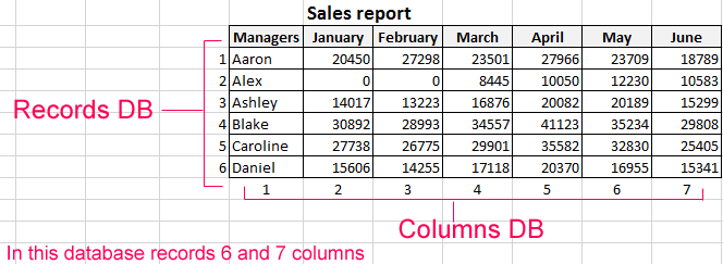
Database Structure — Excel table

Database — a data set distributed in rows and columns for easily searching, organizing and editing. How to make the database in Excel?

All information in the database is contained in the records and fields:

• Record is database (DB) line, which includes information about one object.
• Field is the column in the database that contains information of the same type about all objects.
• Records and database fields correspond to the rows and columns of a standard Microsoft Excel spreadsheet.

If you know how to do a simple table, then creating a database will not be difficult.



Creating DB in Excel: step by step instructions

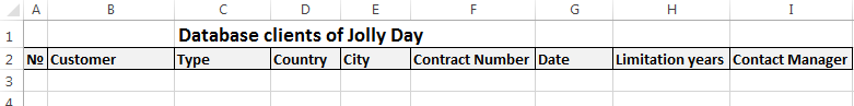
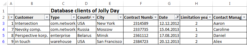
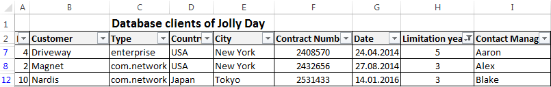
Step by step to create a database in Excel. Our challenge is to form a client database. For several years, the company has several dozens of regular customers. It is necessary to monitor the contract term, the areas of cooperation and to know contacts, data communications, etc.

How to create a customer database in Excel:

1. Enter the name of the database field (column headings).



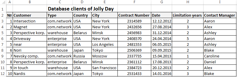
2. Enter data into the database. We are keeping order in the format of the cells. If it is a numerical format so it should be the same numerical format in the entire column. Data are entered in the same way as in a simple table. If the data in a certain cell is the sum on the values of other cells, then create formula.



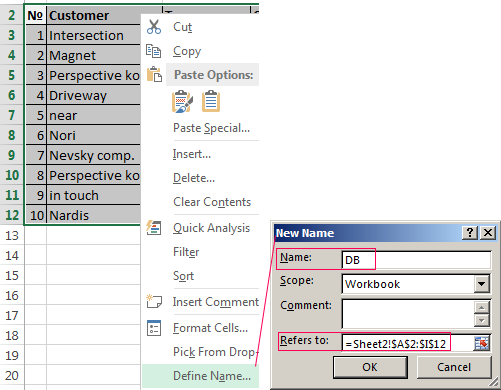
3. To use the database turn to tools «DATA».



4. Assign the name of the database. Select the range of data — from the first to the last cell. Right mouse button — the name of the band. We give any name. Example — DB. Check that the range was correct.

The main work of information entering into the DB is made. For easy using this information it is necessary to pick out the needful information, filter and sort the data.

How to maintain a database in Excel

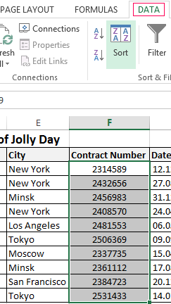
To simplify the search for data in the database, we’ll order them. Tool «Sort» is suitable for this purpose.

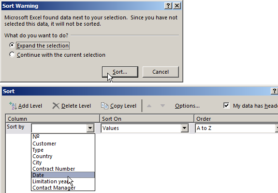
1. Select the range you want to sort. For the purposes of our fictitious company the column «Date». Call the tool «Sort».



2. Then system offers automatically expand the selected range. We agree. If we sort the data of only one column and the rest will leave in place so the information will be wrong. Then the menu will open parameters where we have to choose the options and sorting values.

The data distributed in the table by the term of the contract.

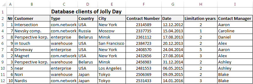
Now, the manager sees to whom it is time to renew the contract and with which companies we continue the partnership.

Database during the company’s activity is growing to epic proportions. Finding the right information is getting harder. To find specific text or numbers you can use:

By simultaneously pressing Ctrl + F or Shift + F5. «Find and Replace» search box appears.

Filtering the data

By filtering the data the program hides all the unnecessary information that user does not need. Data is in the table, but invisible. At any time, data can be recovered.

There are 2 filters which are often used In Excel:

• AutoFilter;
• filter on the selected range.

AutoFilter offers the user the option to choose from a pre-filtering list.

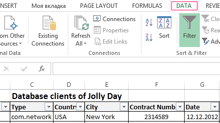
1. On the «DATA» tab, click the button «Filter».



2. Down arrows are appearing after clicking in the header of the table. They signal the inclusion of «AutoFilter».
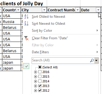
3. Click on the desired column direction to select a filter setting. In the drop-down list appears all the contents of the field. If you want to hide some elements reset the birds in front of them.



4. Press «OK». In the example we hide clients who have concluded contracts in the past and the current year.



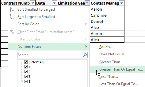
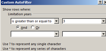
5. To set a condition to filter the field type «Greater Than», «Less Than», «Equals», etc. values, select the command «Number Filters» in the filter list.



6. If we want to see clients in a customer table whom we signed a contract for 3 years or more, enter the appropriate values in the AutoFilter menu.

Done!

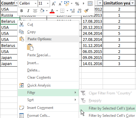
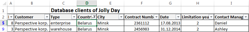
Let’s experiment with the values filtered by the selected cells. For example, we need to leave the table only with those companies that operate in Belarus.

1. Select the data with information which should remain prominent in the database. In our case, we find the column country — «РБ «. We click on the cell with right-click.



2. Perform a sequence command: «Filter»–«Filter by Selected Cell’s Value». Done.

Sum can be found using different parameters if the database contains financial information:

• the sum of (summarize data);
• count (count the number of cells with numerical data);
• average (arithmetic mean count);
• maximum and minimum values in the selected range;
• product (the result of multiplying the data);
• standard deviation and variance of the sample.

Using the financial information in the database:

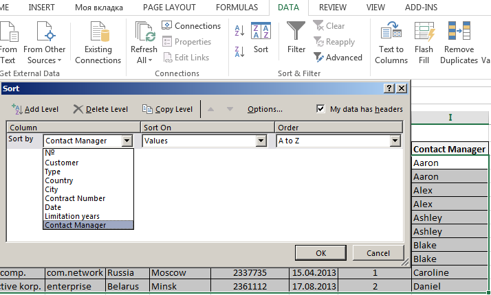
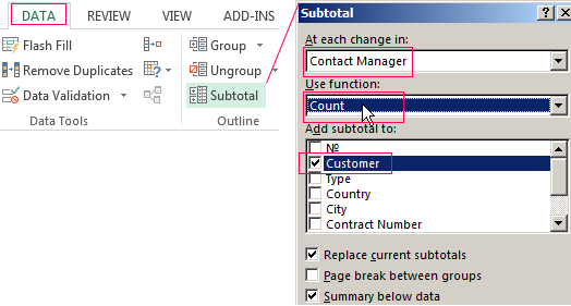
1. Then the menu will open parameters where we have to choose the options and sorting values «Contact Manager».



2. Select the database range. Go to the tab «DATA» — «Subtotal».



3. Select the calculation settings In the dialog box.

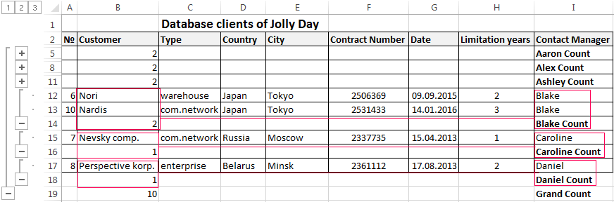
Tools on the «DATA» tab allows to segment the DB. Sort information in terms with relevance to company goals. Isolation of purchasers of goods groups help to promote the marketing of the product.

Prepared sample templates for conducting client base segment:

1. Template for manager which allows monitors the result of outgoing calls to customers download.
2. The simplest template. Customer in Excel free template database download.
3. Example database from this article download example.

Templates can be adjusted for your needs: reduce, expand, and edit.

303

303 people found this article helpful

How to Create a Database in Excel

Track contacts, collections, and other data

Updated on January 30, 2021

What to Know

• Enter data in the cells in columns and rows to create a basic database.
• If using headers, enter them into the first cell in each column.
• Do not leave any rows blank within the database.

This article explains how to create a database in Excel for Microsoft 365, Excel 2019, Excel 2016, Excel 2013, Excel 2010, Excel for Mac, Excel for Android, and Excel Online.

Enter the Data

The basic format for storing data in an Excel database is a table. Once a table has been created, use Excel’s data tools to search, sort, and filter records in the database to find specific information.

To follow along with this tutorial, enter the data as it is shown in the image above.

Enter the Student IDs Quickly

1. Type the first two ID’s, ST348-245 and ST348-246, into cells A5 and A6, respectively.
2. Highlight the two ID’s to select them.
3. Drag the fill handle to cell A13.

The rest of the Student ID’s are entered into cells A6 to A13 correctly.

Enter Data Correctly

When entering the data, it is important to ensure that it is entered correctly. Other than row 2 between the spreadsheet title and the column headings, do not leave any other blank rows when entering your data. Also, make sure that you don’t leave any empty cells.

Data errors caused by incorrect data entry are the source of many problems related to data management. If the data is entered correctly initially, the program is more likely to give you back the results you want.

Rows Are Records

Each row of data in a database is known as a record. When entering records, keep these guidelines in mind:

• Do not leave any blank rows in the table. This includes not leaving a blank row between the column headings and the first row of data.
• A record must contain data about only one specific item.
• A record must also contain all the data in the database about that item. There can’t be information about an item in more than one row.

Columns Are Fields

While rows in an Excel database are referred to as records, the columns are known as fields. Each column needs a heading to identify the data it contains. These headings are called field names.

• Field names are used to ensure that the data for each record is entered in the same sequence.
• Data in a column must be entered using the same format. If you start entering numbers as digits (such as 10 or 20), keep it up. Don’t change partway through and begin entering numbers as words (such as ten or twenty). Be consistent.
• The table must not contain any blank columns.

Create the Table

Once the data has been entered, it can be converted into a table. To convert data into a table:

1. Highlight the cells A3 to E13 in the worksheet.
2. Select the Home tab.
3. Select Format as Table to open the drop-down menu.
4. Choose the blue Table Style Medium 9 option to open the Format as Table dialog box.
5. While the dialog box is open, cells A3 to E13 on the worksheet are surrounded by a dotted line.
6. If the dotted line surrounds the correct range of cells, select OK in the Format as Table dialog box.
7. If the dotted line does not surround the correct range of cells, highlight the correct range in the worksheet and then select OK in the Format as Table dialog box.

Drop-down arrows are added beside each field name, and the table rows are formatted in alternating light and dark blue.

Use the Database Tools

Once you have created the database, use the tools located under the drop-down arrows beside each field name to sort or filter your data.

Sort Data

1. Select the drop-down arrow next to the Last Name field.
2. Select Sort A to Z to sort the database alphabetically.
3. Once sorted, Graham J. is the first record in the table, and Wilson R is the last.

Filter Data

1. Select the drop-down arrow next to the Program field.
2. Select the checkbox next to Select All to clear all check boxes.
3. Select the checkbox next to Business to add a check mark to the box.
4. Select OK.
5. Only two students, G. Thompson and F. Smith are visible because they are the only two students enrolled in the business program.
6. To show all records, select the drop-down arrow next to the Program field and select Clear Filter from «Program.»

Expand the Database

To add additional records to your database:

1. Place your mouse pointer over the small dot in the bottom right-hand corner of the table.
2. The mouse pointer changes into a two-headed arrow.
3. Press and hold the right mouse button and drag the pointer down to add a blank row to the bottom of the database.
4. Add the following data to this new row:
   Cell A14: ST348-255
   Cell B14: Christopher
   Cell C14: A.
   Cell D14: 22
   Cell E14: Science

Complete the Database Formatting

1. Highlight cells A1 to E1 in the worksheet.
2. Select Home.
3. Select Merge and Center to center the title.
4. Select Fill Color to open the fill color drop-down list.
5. Choose Blue, Accent 1 from the list to change the background color in cells A1 to E1 to dark blue.
6. Select Font Color to open the font color drop-down list.
7. Choose White from the list to change the text color in cells A1 to E1 to white.
8. Highlight cells A2 to E2 in the worksheet.
9. Select Fill Color to open the fill color drop-down list.
10. Choose Blue, Accent 1, Lighter 80 from the list to change the background color in cells A2 to E2 to light blue.
11. Highlight cells A4 to E14 in the worksheet.
12. Select Center to center align the text in cells A14 to E14.

Database Functions

Syntax: Dfunction(Database_arr , Field_str|num , Criteria_arr)

Where Dfunction is one of the following:

• DAVERAGE
• DCOUNT
• DCOUNTA
• DGET
• DMAX
• DMIN
• DPRODUCT
• DSTDEV
• DSTDEVP
• DSUM
• DVAR
• DVARP

Type: Database

Database functions are convenient when Google Sheets is used to maintain structured data, like a database. Each database function, Dfunction, computes the corresponding function on a subset of a cell range regarded as a database table. Database functions take three arguments:

• Database_arr is a range, an embedded array, or an array generated by an array expression. It is structured so that each row after Row 1 is a database record, and each column is a database field. Row 1 contains the labels for each field.
• Field_str|num indicates which column (field) contains the values to be averaged. This can be expressed as either the field name (text string) or the column number, where the left-most column would be represented as 1.
• Criteria_arr is a range, an embedded array, or an array generated by an array expression. It is structured such that the first row contains the field name(s) to which the criterion (criteria) will be applied, and subsequent rows contain the conditional test(s).

The first row in Criteria specifies field names. Every other row in Criteria represents a filter, a set of restrictions on the corresponding fields. Restrictions are described using Query-by-Example notation and include a value to match or a comparison operator followed by a comparison value. Examples of restrictions are: «Chocolate», «42», «>= 42», and «<> 42». An empty cell means no restriction on the corresponding field.

A filter matches a database row if all the filter restrictions (the restrictions in the filter’s row) are met. A database row (a record) satisfies Criteria if at least one filter matches it. A field name may appear more than once in the Criteria range to allow multiple restrictions that apply simultaneously (for example, temperature >= 65 and temperature <= 82).

DGET is the only database function that doesn’t aggregate values. DGET returns the value of the field specified in the second argument (similarly to a VLOOKUP) only when exactly one record matches Criteria; otherwise, it returns an error indicating no matches or multiple matches.

Thanks for letting us know!

Get the Latest Tech News Delivered Every Day

Subscribe

As a business owner or project manager, you’re handling most things on your own at the beginning. Marketing, brand strategy, client communication—the list goes on! But there’s one thing you must have to scale: data management. 

Databases aren’t just for big companies with hundreds or thousands of clients and products. It’s for anyone who wants to put manual work on autopilot, so they can track, retrieve, and protect all types of information. 

If you’re using Excel as a temporary tool to import and export work, try ClickUp! You’ll have free access to actionable reports, change records, and powerful integrations—without the tech headache.

How to Create a Database in Excel

If you’ve struggled with creating or maintaining a database, you might feel every day is Day One because tracking is a labor-intense task in Excel.

So let’s learn how to create a database in Excel to sidestep the complexities and get to the good part: interacting with our data!

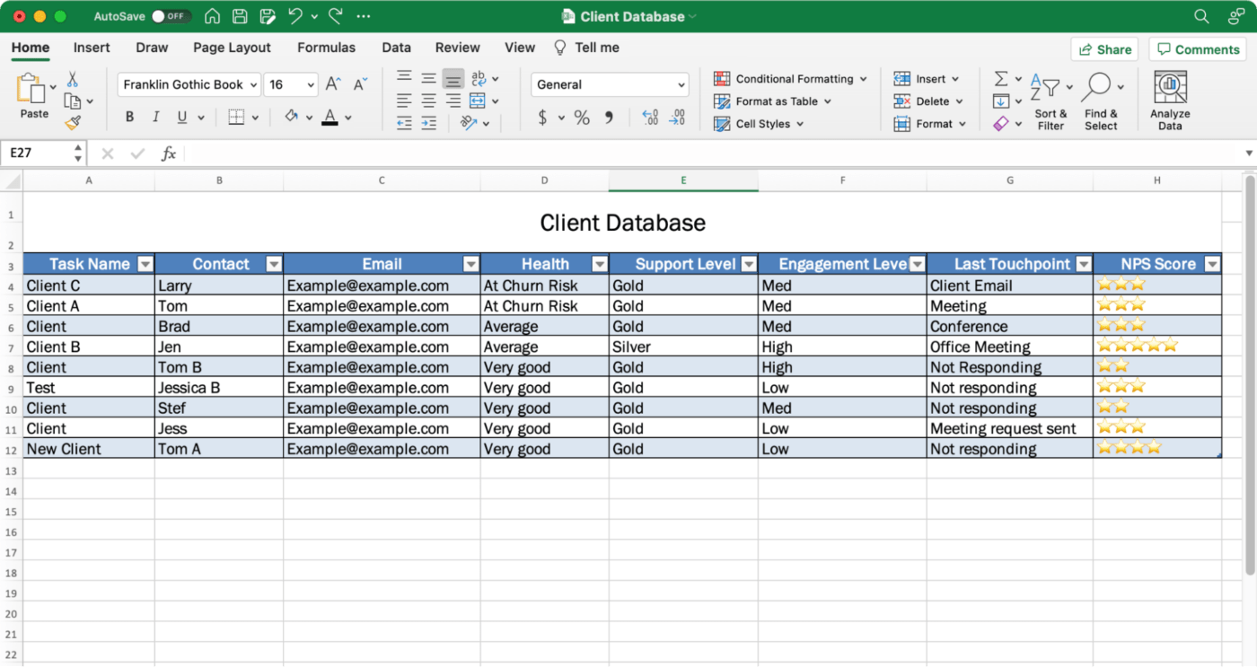
In this guide, we use Microsoft Word for Mac Version 16.54 to demonstrate a Client Management database. The features mentioned may look different if you’re on another platform or version.

Step 1: Set up a data spreadsheet framework 

Open an Excel spreadsheet, place your cursor in the A1 cell, and type in your database title. 

Go to the next row, and from left to right, use the Tab key to move through your blank database to add your column headers. Feel free to use this list as inspiration for your spreadsheet:

• Client Name
• Contact Name
• Email
• Health Level (drop down)
• Support Level (drop down)
• Engagement Level (drop down)
• Last Touchpoint
• NPS Score

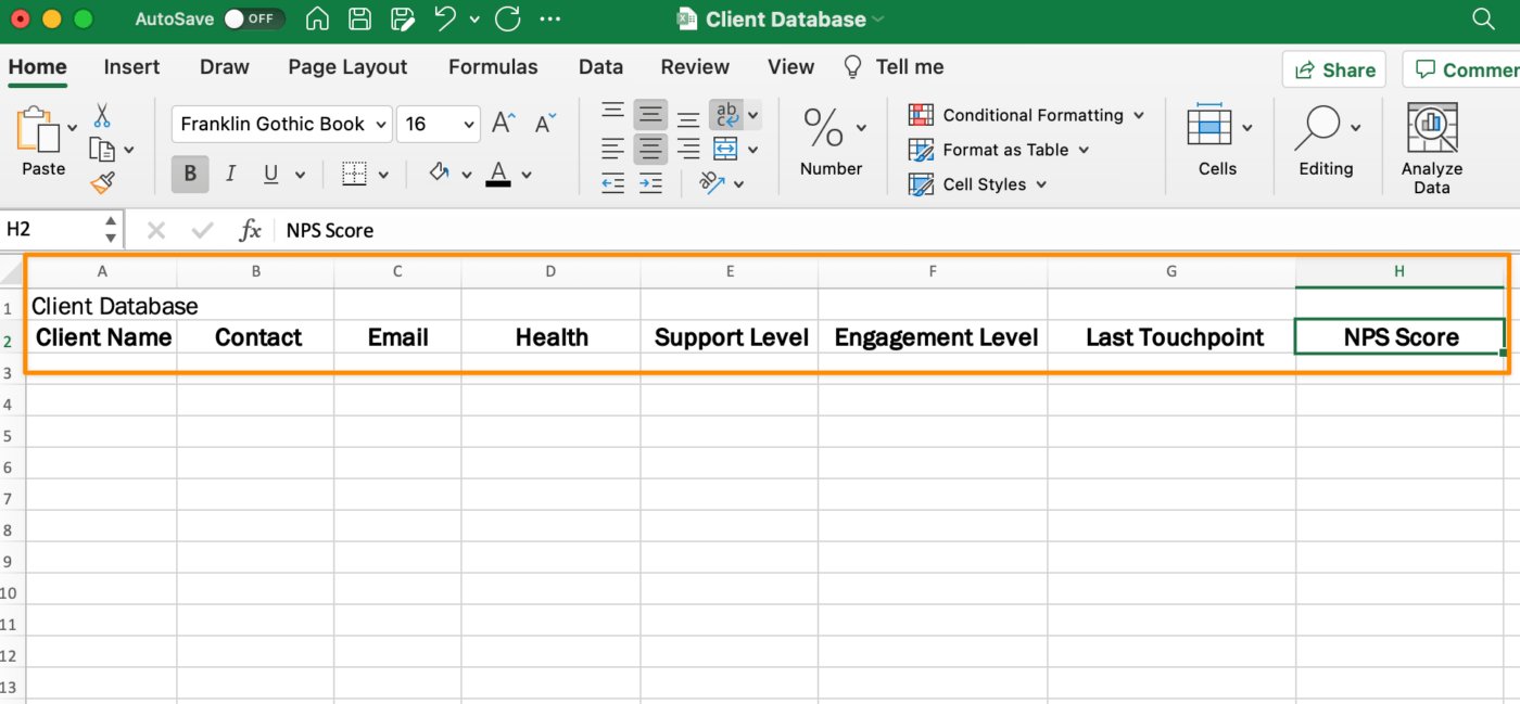
Go back to your database title and highlight the first row up to the last column of your table. From the Home tab in the menu toolbar, click Merge & Center. 

Step 2: Add or import data

You have the option to manually enter data or import data from an existing database using the External Data tab. Keep in mind you will have a database field for certain columns. Here’s another list for inspiration: 

• Client Name
• Contact Name
• Email
• Health Level (drop down: At Churn Risk, Average, Very Good)
• Support Level (drop down: Gold, Silver)
• Engagement Level (drop down: High, Medium, Low)
• Last Touchpoint
• NPS Score

Bulk editing can be scary in Excel, so take this part slow!

Step 3: Convert your data into a table

Now let’s convert your data into a data model table!

Click inside any cell with data (avoid blank rows), and from the menu toolbar, go to Insert tab > Table. All the rows and columns with your data will be selected. We don’t want the title to be included in the table, so we have to manually highlight the table without the title. Then, click OK. 

Step 4: Format the table 

From the Table tab in the menu toolbar, choose any table design to fit your preference. Knowing where your table will be displayed will help you decide. Looking at a spreadsheet on a big screen in a conference room versus a 16-inch laptop makes all the difference to a person’s experience with the data!

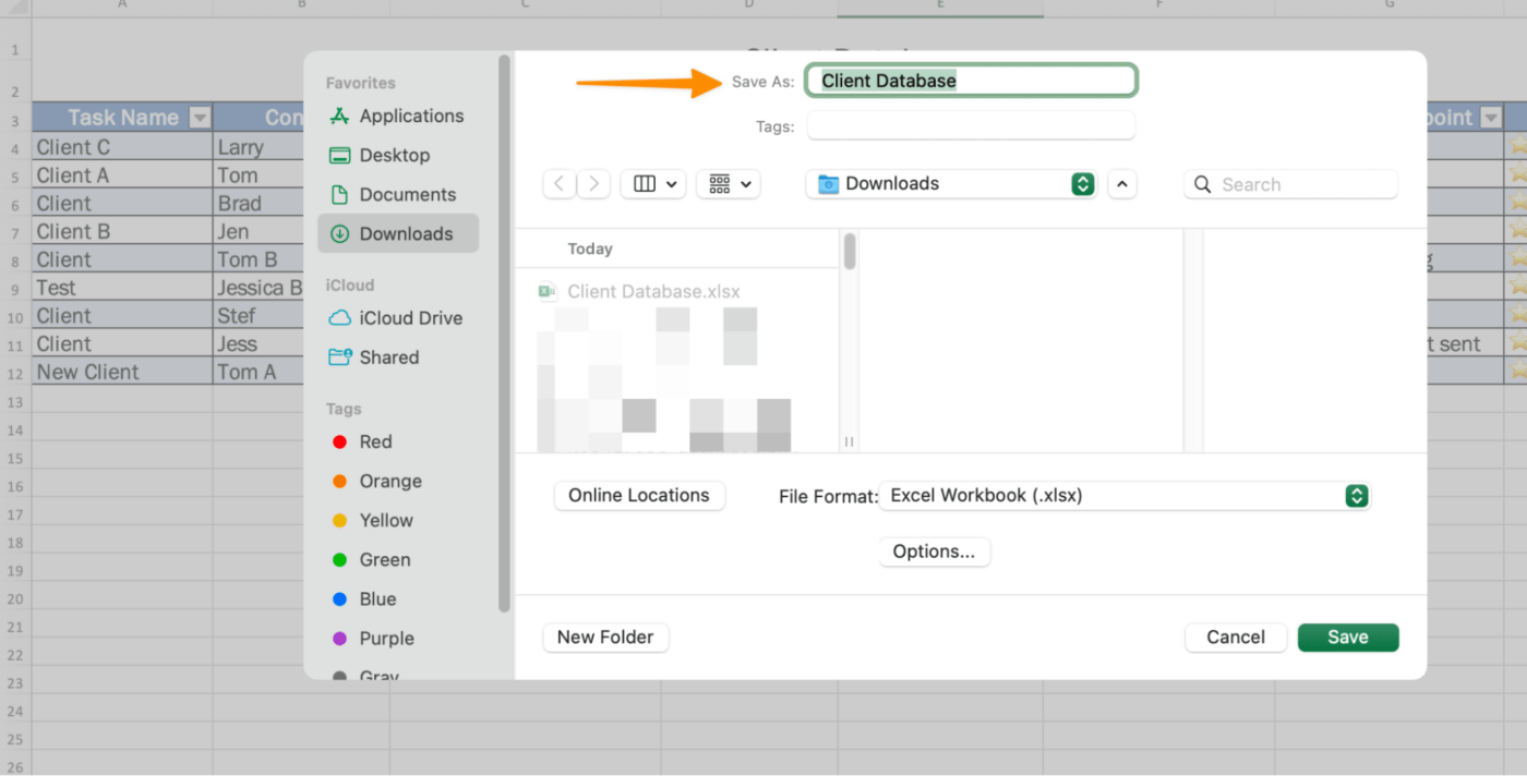
Step 5: Save your database spreadsheet

Finally, save your spreadsheet because you will have to come back and manually edit your database multiple times a day or week with the latest information. Set up Future You for success, so you don’t risk starting over! 

Go to File > Save As > Name your database > click Save. 

Free Database Templates

Check out these pre-made templates to jumpstart your database-building task!

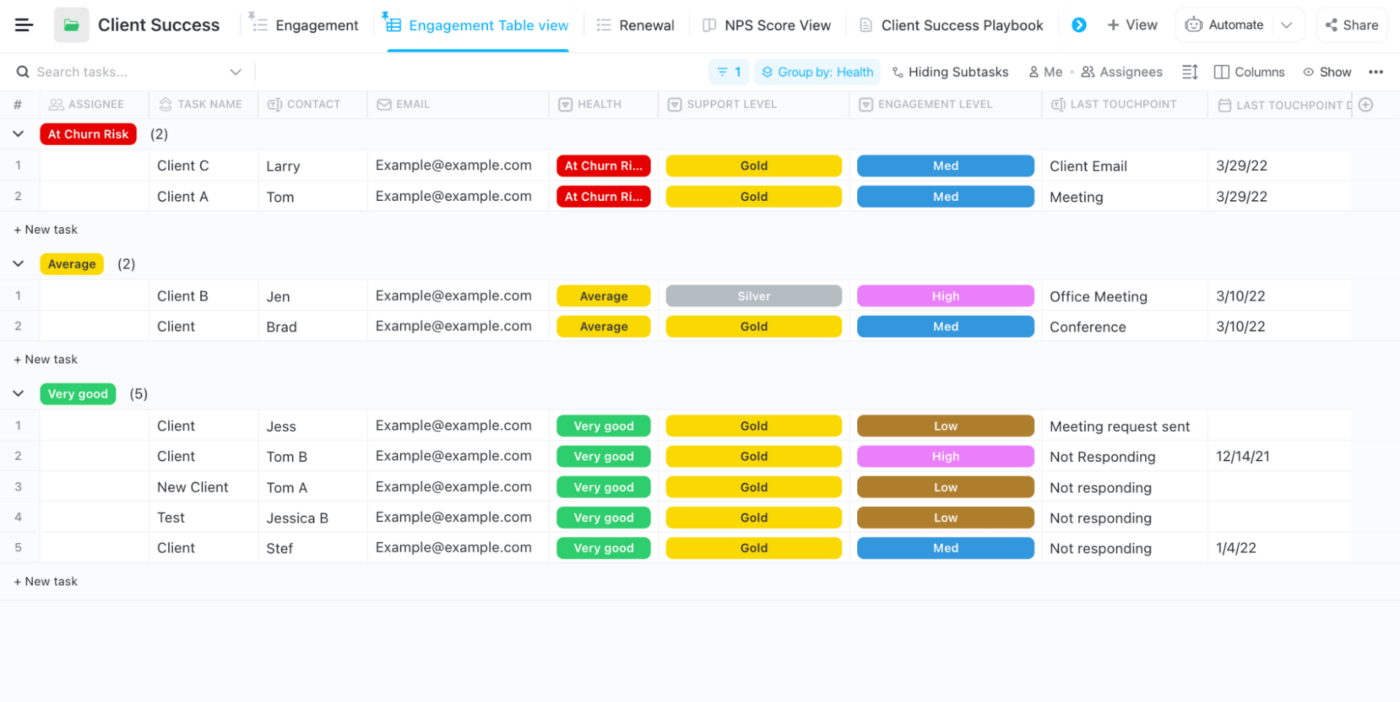
1. Client Success Template by ClickUp 

2. Excel’s Inventory List Template

3. Excel’s Warehouse Inventory Template

4. Excel’s Contact List Template

Related Resources:

• Excel Alternatives
• How to Create a Project Timeline in Excel
• How to Make a Calendar in Excel
• How to create Gantt charts in Excel
• How to create a Kanban board in Excel
• How to create a burndown chart in Excel
• How to create a flowchart in Excel
• How to Create an Org Chart in Excel
• How to Make a Graph in Excel
• How to Make a KPI Dashboard in Excel

How to Make a Database With ClickUp’s Table View

If you’re in a position where you’ll be using the database daily—meaning it’s an essential tool to get your work done—Excel won’t support your growth long-term.

Excel isn’t a database software built for the modern workplace. Workers are on-the-go and mobile-first. An Excel workflow sucks up time that should be spent making client connections and focusing on needle-moving tasks. 

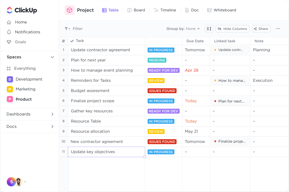
If you need a solution to bring project and client management under one roof, try ClickUp! 

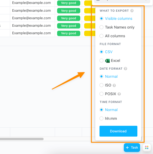
The process of building a simple but powerful database is easy in ClickUp. Import your work from almost anywhere with ClickUp’s free Excel and CSV import feature. Or vice versa! After you build a database in ClickUp, you can export it as an Excel or CSV file.

Is end-to-end security a non-negotiable term for your database tool? Same for ClickUp!

ClickUp has one of the strictest policies in our industry to ensure your data never gets into the hands of third parties. If you have a security question or concern, please feel free to ask us any time! 

Using a Table view in ClickUp is like using an Excel spreadsheet, only: 

• Data organization possibilities are endless with ClickUp Custom Fields 
• Advanced filtering options make searching for data and activity stress-free
• Tasks in ClickUp empower you to plan, organize, and collaborate on any project
• Native or third-party integrations in ClickUp connect your favorite tools together
• Formatting options take fewer clicks to view only the data you need right away 

There’s a stocked library of free Sales and CRM ClickUp templates for you to play in a digital sandbox with data examples if you want to see the potential of ClickUp—or get a few database ideas for your own.

We hope you feel more comfortable in the database-building process. You have other options than Excel to move your business closer to your goals.