
Many users are actively using Excel to generate reports for their subsequent editing. Reports are using for easy viewing of information and a complete control over data management during working with the program.
Table is the interface of the workspace of the program. A relational database structures the information in the rows and columns. Despite the fact that the standard package MS Office has a standalone application for creating and maintaining databases named Microsoft Access, users are actively using Microsoft Excel for the same purpose. After all program features allow you to: sort; format; filter; edit; organize and structure the information.
That is all that you need for working with databases. The only caveat: the Excel program is a versatile analytical tool that is more suitable for complex calculations, computations, sorting, and even for storage structured data, but in small amounts (no more than one million records in the same table, in the 2010 version).
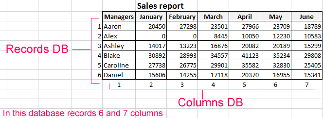
Database Structure — Excel table
Database — a data set distributed in rows and columns for easily searching, organizing and editing. How to make the database in Excel?
All information in the database is contained in the records and fields:
- Record is database (DB) line, which includes information about one object.
- Field is the column in the database that contains information of the same type about all objects.
- Records and database fields correspond to the rows and columns of a standard Microsoft Excel spreadsheet.
If you know how to do a simple table, then creating a database will not be difficult.
Creating DB in Excel: step by step instructions
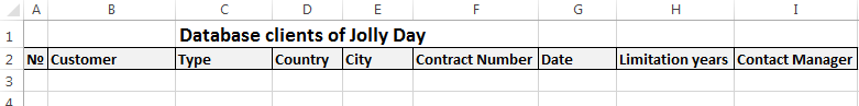
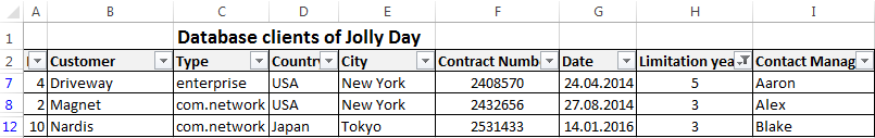
Step by step to create a database in Excel. Our challenge is to form a client database. For several years, the company has several dozens of regular customers. It is necessary to monitor the contract term, the areas of cooperation and to know contacts, data communications, etc.
How to create a customer database in Excel:
- Enter the name of the database field (column headings).
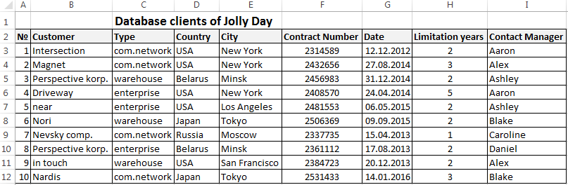
- Enter data into the database. We are keeping order in the format of the cells. If it is a numerical format so it should be the same numerical format in the entire column. Data are entered in the same way as in a simple table. If the data in a certain cell is the sum on the values of other cells, then create formula.
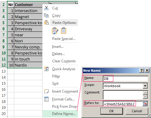
- To use the database turn to tools «DATA».
- Assign the name of the database. Select the range of data — from the first to the last cell. Right mouse button — the name of the band. We give any name. Example — DB. Check that the range was correct.
The main work of information entering into the DB is made. For easy using this information it is necessary to pick out the needful information, filter and sort the data.
How to maintain a database in Excel
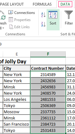
To simplify the search for data in the database, we’ll order them. Tool «Sort» is suitable for this purpose.
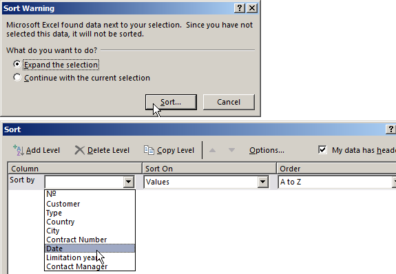
- Select the range you want to sort. For the purposes of our fictitious company the column «Date». Call the tool «Sort».
- Then system offers automatically expand the selected range. We agree. If we sort the data of only one column and the rest will leave in place so the information will be wrong. Then the menu will open parameters where we have to choose the options and sorting values.
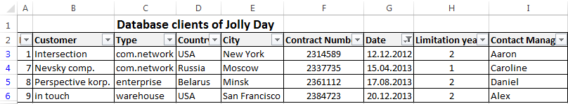
The data distributed in the table by the term of the contract.
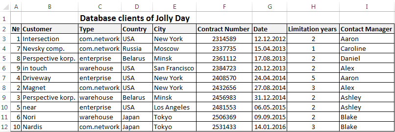
Now, the manager sees to whom it is time to renew the contract and with which companies we continue the partnership.
Database during the company’s activity is growing to epic proportions. Finding the right information is getting harder. To find specific text or numbers you can use:
By simultaneously pressing Ctrl + F or Shift + F5. «Find and Replace» search box appears.
Filtering the data
By filtering the data the program hides all the unnecessary information that user does not need. Data is in the table, but invisible. At any time, data can be recovered.
There are 2 filters which are often used In Excel:
- AutoFilter;
- filter on the selected range.
AutoFilter offers the user the option to choose from a pre-filtering list.
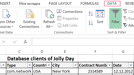
- On the «DATA» tab, click the button «Filter».
- Down arrows are appearing after clicking in the header of the table. They signal the inclusion of «AutoFilter».
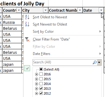
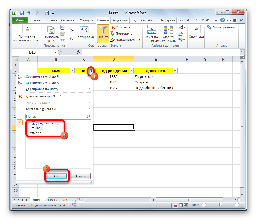
- Click on the desired column direction to select a filter setting. In the drop-down list appears all the contents of the field. If you want to hide some elements reset the birds in front of them.
- Press «OK». In the example we hide clients who have concluded contracts in the past and the current year.
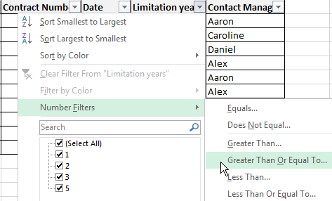
- To set a condition to filter the field type «Greater Than», «Less Than», «Equals», etc. values, select the command «Number Filters» in the filter list.
- If we want to see clients in a customer table whom we signed a contract for 3 years or more, enter the appropriate values in the AutoFilter menu.
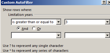
Done!
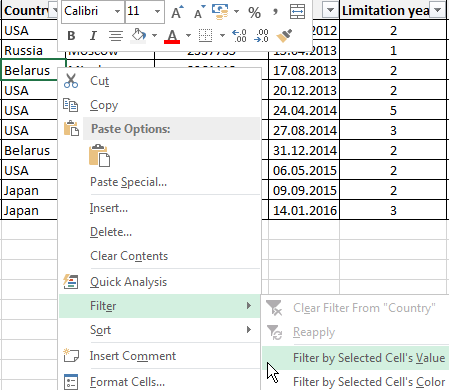
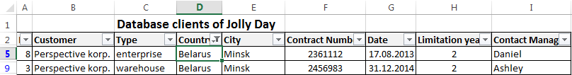
Let’s experiment with the values filtered by the selected cells. For example, we need to leave the table only with those companies that operate in Belarus.
- Select the data with information which should remain prominent in the database. In our case, we find the column country — «РБ «. We click on the cell with right-click.
- Perform a sequence command: «Filter»–«Filter by Selected Cell’s Value». Done.
Sum can be found using different parameters if the database contains financial information:
- the sum of (summarize data);
- count (count the number of cells with numerical data);
- average (arithmetic mean count);
- maximum and minimum values in the selected range;
- product (the result of multiplying the data);
- standard deviation and variance of the sample.
Using the financial information in the database:
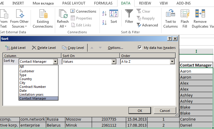
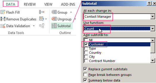
- Then the menu will open parameters where we have to choose the options and sorting values «Contact Manager».
- Select the database range. Go to the tab «DATA» — «Subtotal».
- Select the calculation settings In the dialog box.
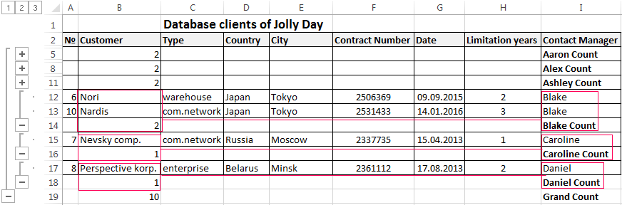
Tools on the «DATA» tab allows to segment the DB. Sort information in terms with relevance to company goals. Isolation of purchasers of goods groups help to promote the marketing of the product.
Prepared sample templates for conducting client base segment:
- Template for manager which allows monitors the result of outgoing calls to customers download.
- The simplest template. Customer in Excel free template database download.
- Example database from this article download example.
Templates can be adjusted for your needs: reduce, expand, and edit.
Содержание
- Процесс создания
- Создание таблицы
- Присвоение атрибутов базы данных
- Сортировка и фильтр
- Поиск
- Закрепление областей
- Выпадающий список
- Вопросы и ответы

В пакете Microsoft Office есть специальная программа для создания базы данных и работы с ними – Access. Тем не менее, многие пользователи предпочитают использовать для этих целей более знакомое им приложение – Excel. Нужно отметить, что у этой программы имеется весь инструментарий для создания полноценной базы данных (БД). Давайте выясним, как это сделать.
Процесс создания
База данных в Экселе представляет собой структурированный набор информации, распределенный по столбцам и строкам листа.
Согласно специальной терминологии, строки БД именуются «записями». В каждой записи находится информация об отдельном объекте.
Столбцы называются «полями». В каждом поле располагается отдельный параметр всех записей.
То есть, каркасом любой базы данных в Excel является обычная таблица.
Создание таблицы
Итак, прежде всего нам нужно создать таблицу.
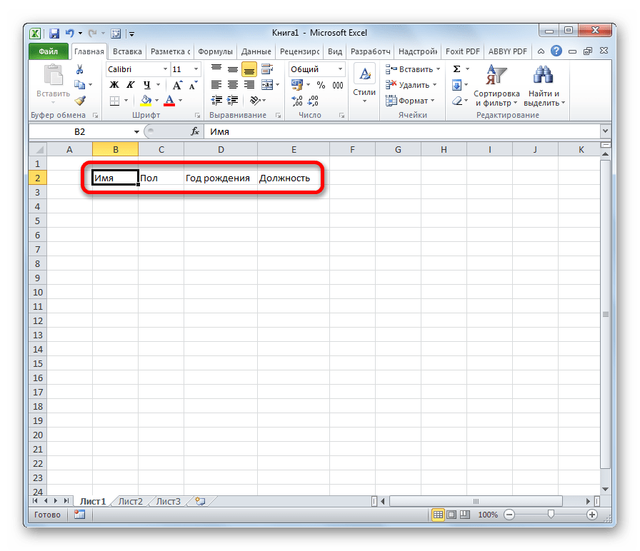
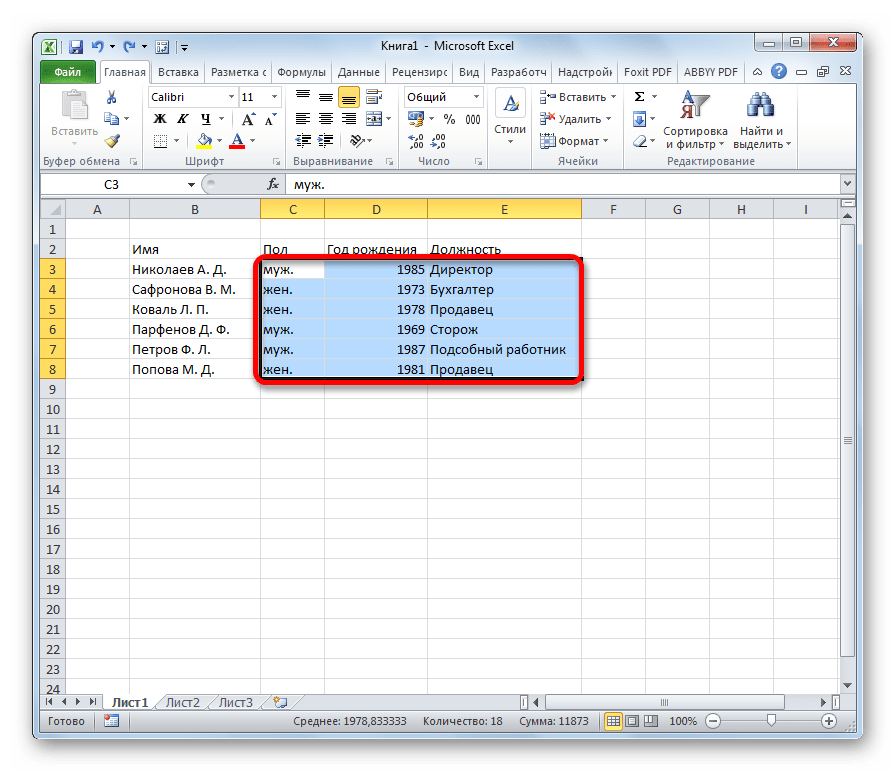
- Вписываем заголовки полей (столбцов) БД.
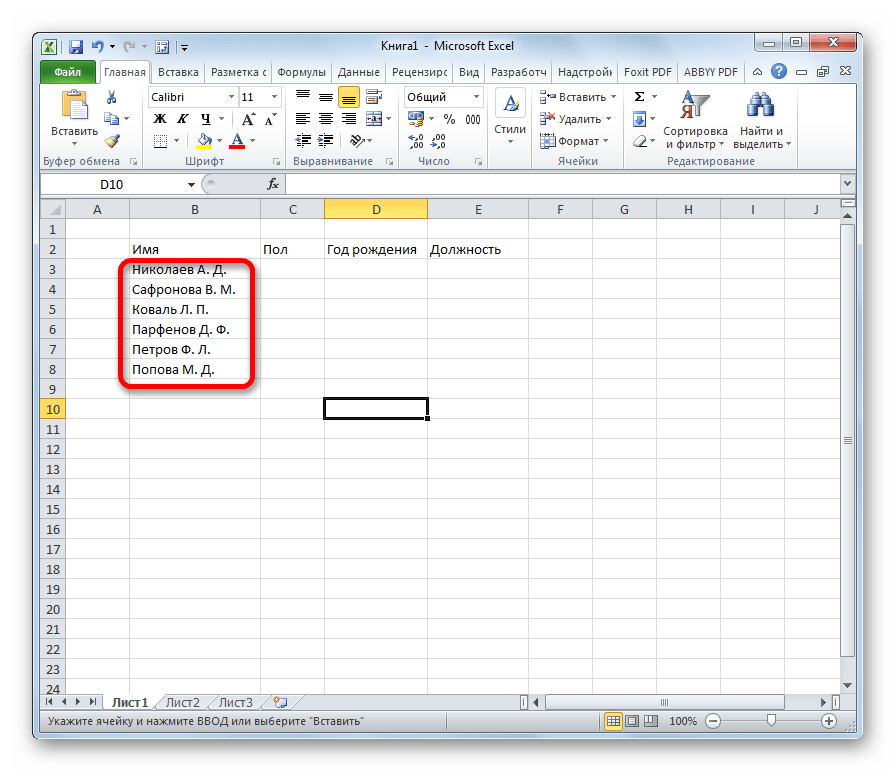
- Заполняем наименование записей (строк) БД.
- Переходим к заполнению базы данными.
- После того, как БД заполнена, форматируем информацию в ней на свое усмотрение (шрифт, границы, заливка, выделение, расположение текста относительно ячейки и т.д.).
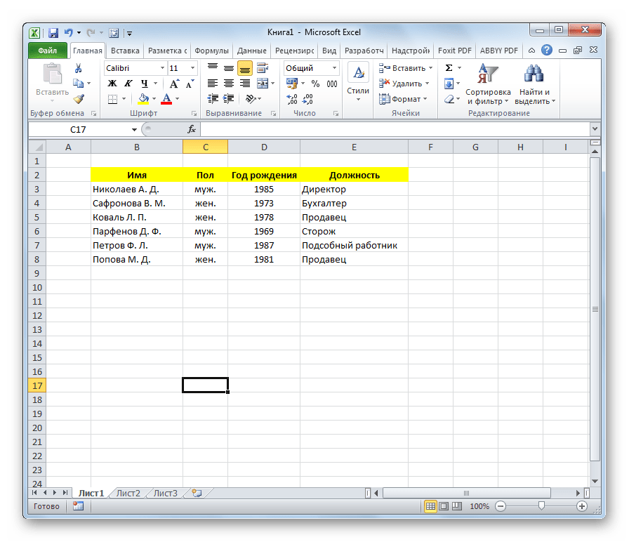
На этом создание каркаса БД закончено.
Урок: Как сделать таблицу в Excel
Присвоение атрибутов базы данных
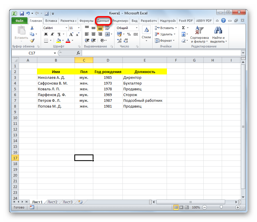
Для того, чтобы Excel воспринимал таблицу не просто как диапазон ячеек, а именно как БД, ей нужно присвоить соответствующие атрибуты.
- Переходим во вкладку «Данные».
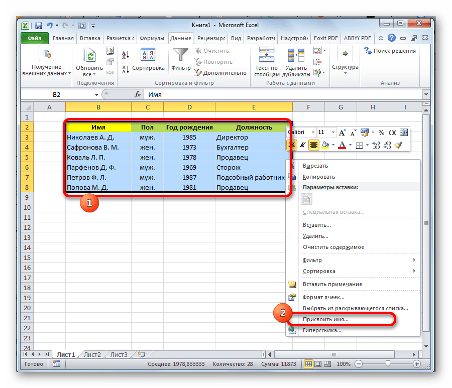
- Выделяем весь диапазон таблицы. Кликаем правой кнопкой мыши. В контекстном меню жмем на кнопку «Присвоить имя…».
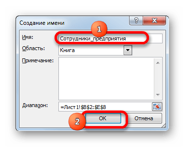
- В графе «Имя» указываем то наименование, которым мы хотим назвать базу данных. Обязательным условием является то, что наименование должно начинаться с буквы, и в нём не должно быть пробелов. В графе «Диапазон» можно изменить адрес области таблицы, но если вы её выделили правильно, то ничего тут менять не нужно. При желании в отдельном поле можно указать примечание, но этот параметр не является обязательным. После того, как все изменения внесены, жмем на кнопку «OK».
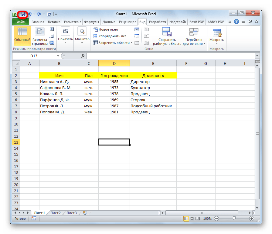
- Кликаем по кнопке «Сохранить» в верхней части окна или набираем на клавиатуре сочетание клавиш Ctrl+S, для того, чтобы сберечь БД на жестком диске или съемном носителе, подключенном к ПК.

Можно сказать, что после этого мы уже имеем готовую базу данных. С ней можно работать и в таком состоянии, как она представлена сейчас, но многие возможности при этом будут урезаны. Ниже мы разберем, как сделать БД более функциональной.
Сортировка и фильтр
Работа с базами данных, прежде всего, предусматривает возможность упорядочивания, отбора и сортировки записей. Подключим эти функции к нашей БД.
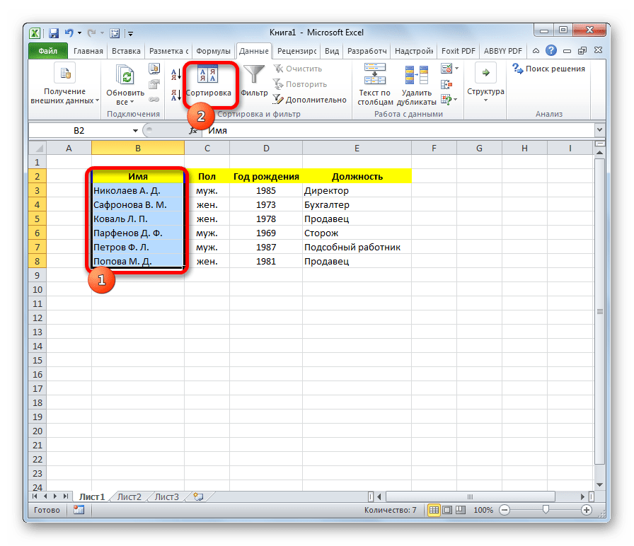
- Выделяем информацию того поля, по которому собираемся провести упорядочивание. Кликаем по кнопке «Сортировка» расположенной на ленте во вкладке «Данные» в блоке инструментов «Сортировка и фильтр».

Сортировку можно проводить практически по любому параметру:
- имя по алфавиту;
- дата;
- число и т.д.
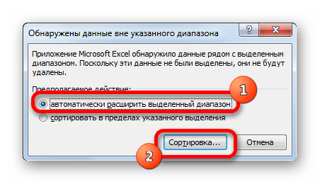
- В следующем появившемся окне будет вопрос, использовать ли для сортировки только выделенную область или автоматически расширять её. Выбираем автоматическое расширение и жмем на кнопку «Сортировка…».
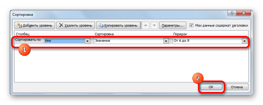
- Открывается окно настройки сортировки. В поле «Сортировать по» указываем имя поля, по которому она будет проводиться.
- В поле «Сортировка» указывается, как именно она будет выполняться. Для БД лучше всего выбрать параметр «Значения».
- В поле «Порядок» указываем, в каком порядке будет проводиться сортировка. Для разных типов информации в этом окне высвечиваются разные значения. Например, для текстовых данных – это будет значение «От А до Я» или «От Я до А», а для числовых – «По возрастанию» или «По убыванию».
- Важно проследить, чтобы около значения «Мои данные содержат заголовки» стояла галочка. Если её нет, то нужно поставить.
После ввода всех нужных параметров жмем на кнопку «OK».

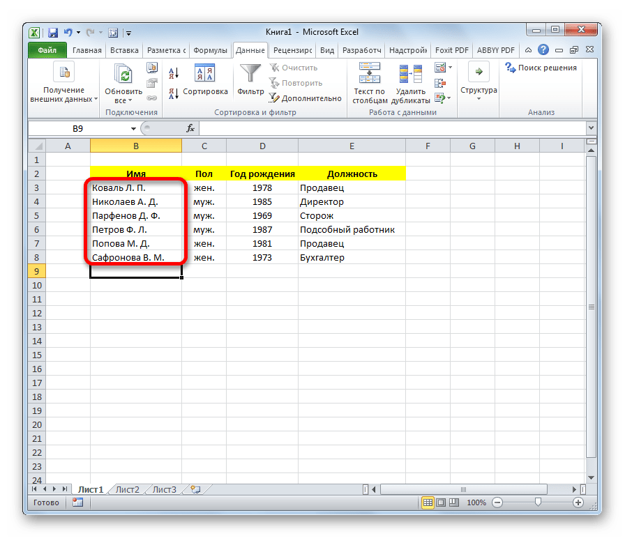
После этого информация в БД будет отсортирована, согласно указанным настройкам. В этом случае мы выполнили сортировку по именам сотрудников предприятия.
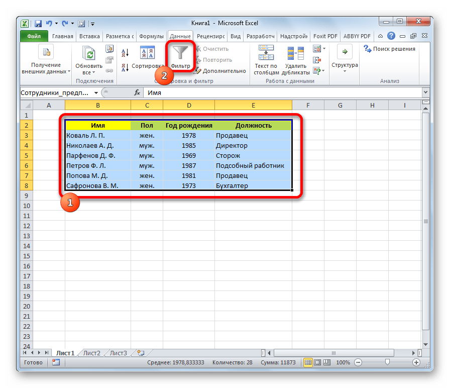
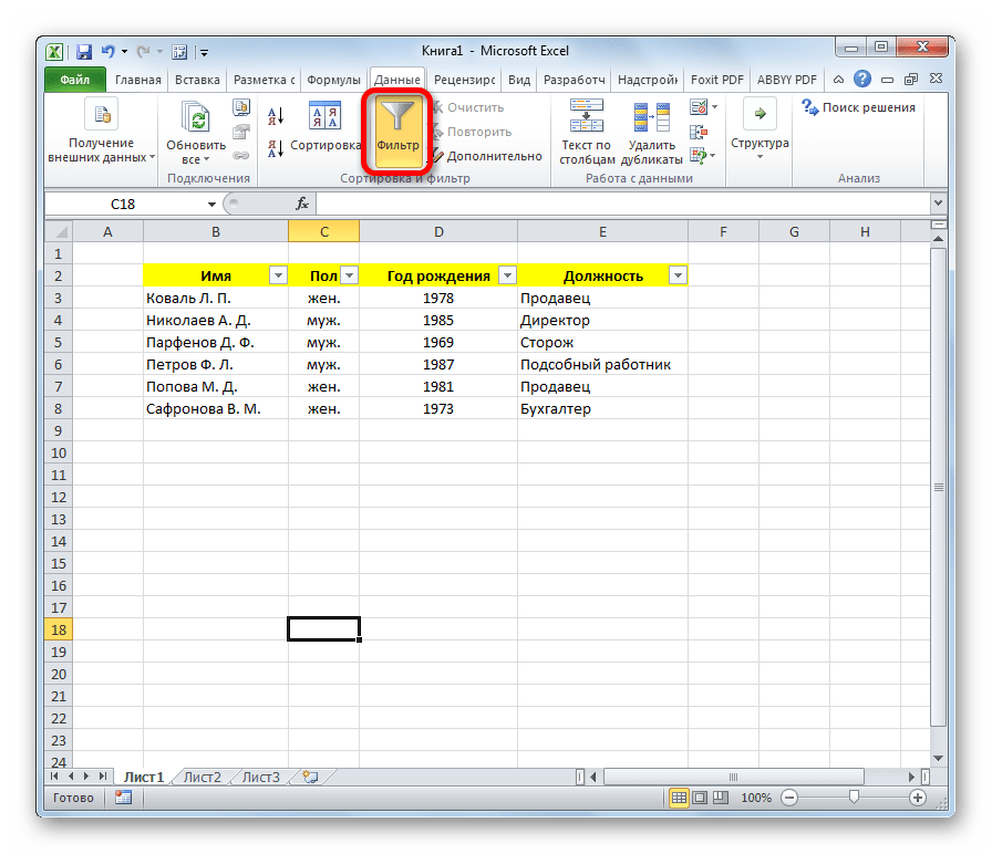
- Одним из наиболее удобных инструментов при работе в базе данных Excel является автофильтр. Выделяем весь диапазон БД и в блоке настроек «Сортировка и фильтр» кликаем по кнопке «Фильтр».
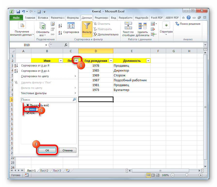
- Как видим, после этого в ячейках с наименованием полей появились пиктограммы в виде перевернутых треугольников. Кликаем по пиктограмме того столбца, значение которого собираемся отфильтровать. В открывшемся окошке снимаем галочки с тех значений, записи с которыми хотим скрыть. После того как выбор сделан, жмем на кнопку «OK».

Как видим, после этого, строки, где содержатся значения, с которых мы сняли галочки, были скрыты из таблицы.
- Для того, чтобы вернуть все данные на экран, кликаем на пиктограмму того столбца, по которому проводилась фильтрация, и в открывшемся окне напротив всех пунктов устанавливаем галочки. Затем жмем на кнопку «OK».
- Для того, чтобы полностью убрать фильтрацию, жмем на кнопку «Фильтр» на ленте.
Урок: Сортировка и фильтрация данных в Excel
Поиск
При наличии большой БД поиск по ней удобно производить с помощь специального инструмента.
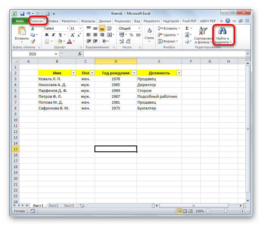
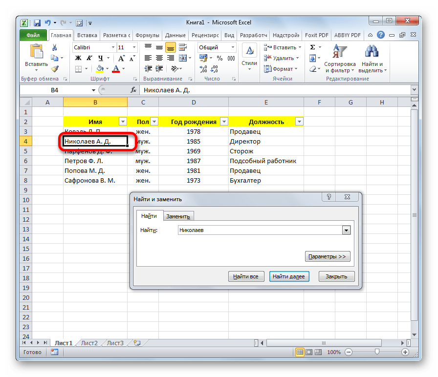
- Для этого переходим во вкладку «Главная» и на ленте в блоке инструментов «Редактирование» жмем на кнопку «Найти и выделить».
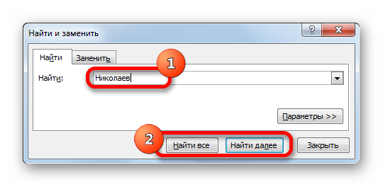
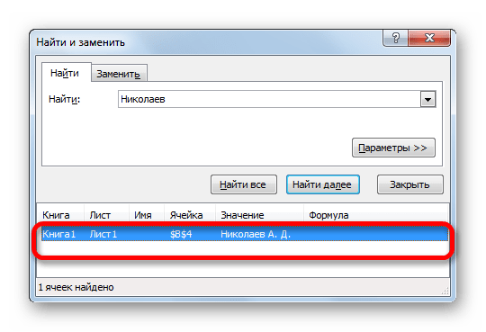
- Открывается окно, в котором нужно указать искомое значение. После этого жмем на кнопку «Найти далее» или «Найти все».
- В первом случае первая ячейка, в которой имеется указанное значение, становится активной.
Во втором случае открывается весь перечень ячеек, содержащих это значение.
Урок: Как сделать поиск в Экселе
Закрепление областей
Удобно при создании БД закрепить ячейки с наименованием записей и полей. При работе с большой базой – это просто необходимое условие. Иначе постоянно придется тратить время на пролистывание листа, чтобы посмотреть, какой строке или столбцу соответствует определенное значение.
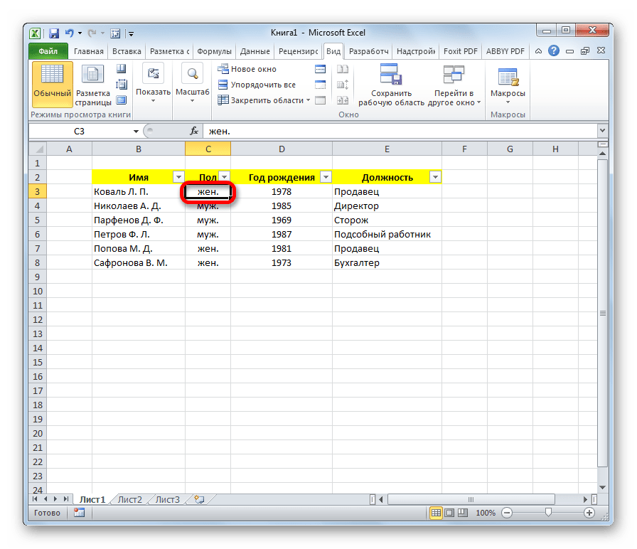
- Выделяем ячейку, области сверху и слева от которой нужно закрепить. Она будет располагаться сразу под шапкой и справа от наименований записей.
- Находясь во вкладке «Вид» кликаем по кнопке «Закрепить области», которая расположена в группе инструментов «Окно». В выпадающем списке выбираем значение «Закрепить области».
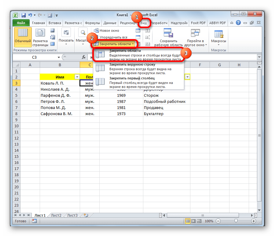
Теперь наименования полей и записей будут у вас всегда перед глазами, как бы далеко вы не прокручивали лист с данными.
Урок: Как закрепить область в Экселе
Выпадающий список
Для некоторых полей таблицы оптимально будет организовать выпадающий список, чтобы пользователи, добавляя новые записи, могли указывать только определенные параметры. Это актуально, например, для поля «Пол». Ведь тут возможно всего два варианта: мужской и женский.
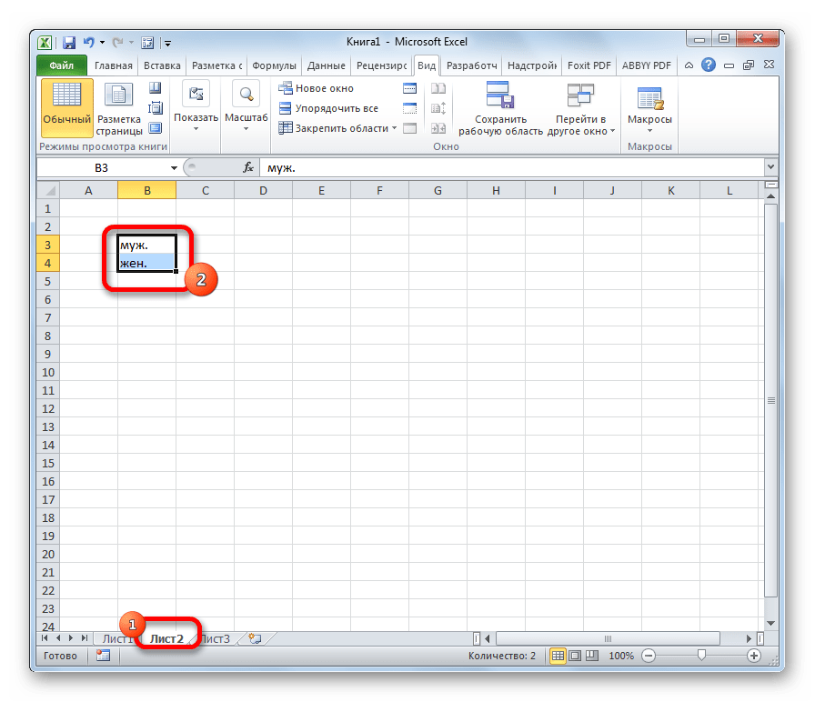
- Создаем дополнительный список. Удобнее всего его будет разместить на другом листе. В нём указываем перечень значений, которые будут появляться в выпадающем списке.
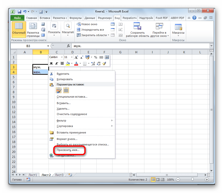
- Выделяем этот список и кликаем по нему правой кнопкой мыши. В появившемся меню выбираем пункт «Присвоить имя…».
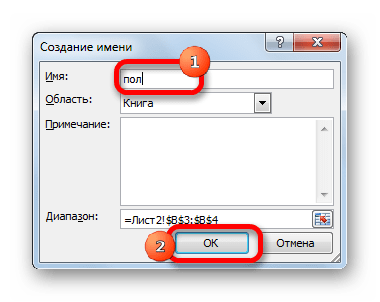
- Открывается уже знакомое нам окно. В соответствующем поле присваиваем имя нашему диапазону, согласно условиям, о которых уже шла речь выше.
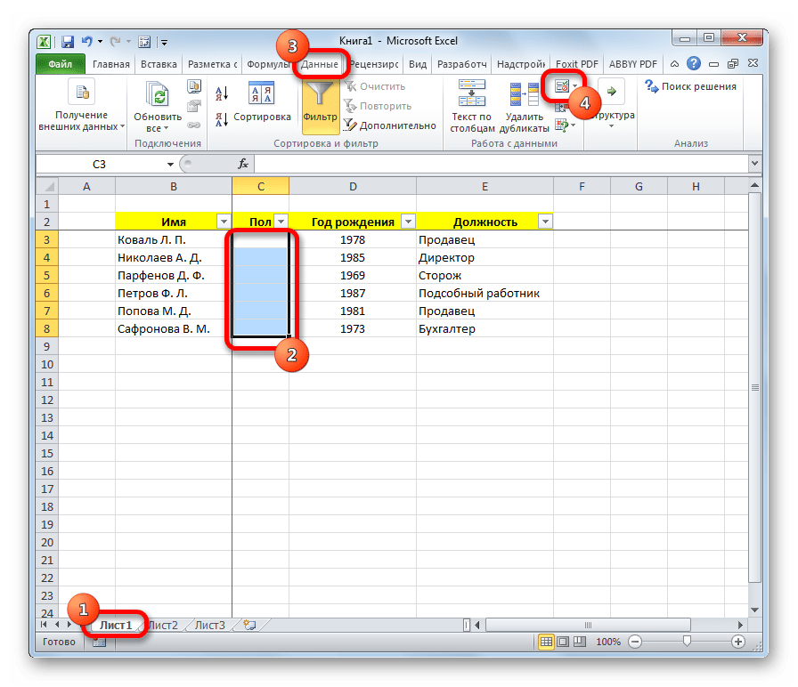
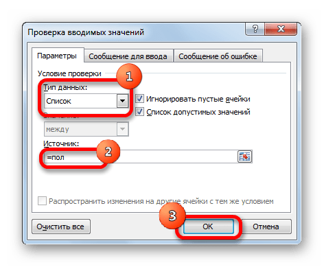
- Возвращаемся на лист с БД. Выделяем диапазон, к которому будет применяться выпадающий список. Переходим во вкладку «Данные». Жмем на кнопку «Проверка данных», которая расположена на ленте в блоке инструментов «Работа с данными».
- Открывается окно проверки видимых значений. В поле «Тип данных» выставляем переключатель в позицию «Список». В поле «Источник» устанавливаем знак «=» и сразу после него без пробела пишем наименование выпадающего списка, которое мы дали ему чуть выше. После этого жмем на кнопку «OK».
Теперь при попытке ввести данные в диапазон, где было установлено ограничение, будет появляться список, в котором можно произвести выбор между четко установленными значениями.
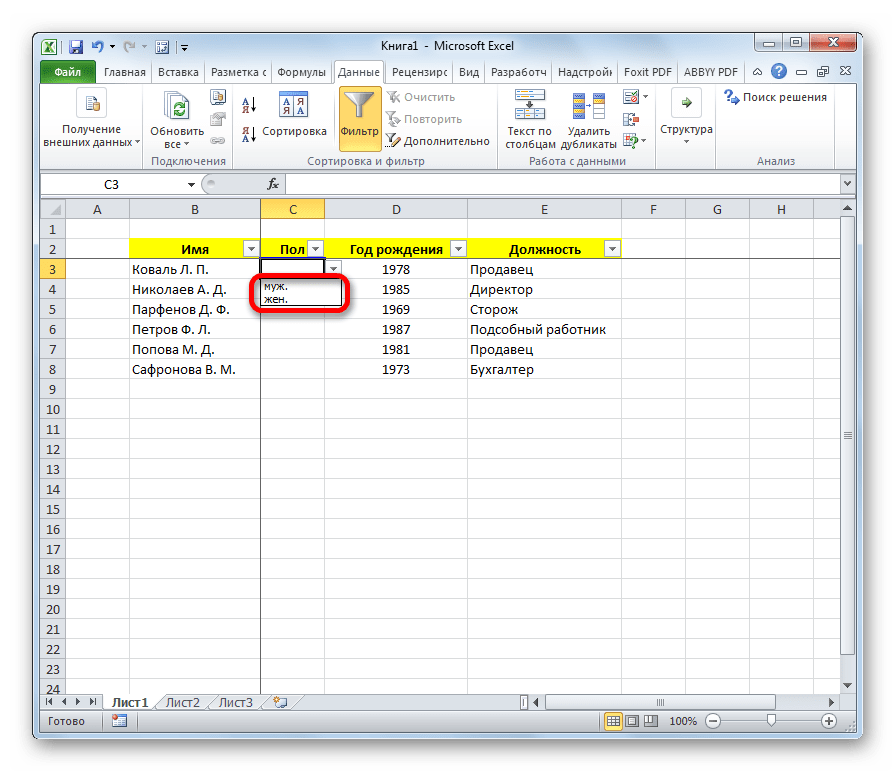
Если же вы попытаетесь написать в этих ячейках произвольные символы, то будет появляться сообщение об ошибке. Вам придется вернутся и внести корректную запись.

Урок: Как сделать выпадающий список в Excel
Конечно, Excel уступает по своим возможностям специализированным программам для создания баз данных. Тем не менее, у него имеется инструментарий, который в большинстве случаев удовлетворит потребности пользователей, желающих создать БД. Учитывая тот факт, что возможности Эксель, в сравнении со специализированными приложениями, обычным юзерам известны намного лучше, то в этом плане у разработки компании Microsoft есть даже некоторые преимущества.
Do you need to create and use a database? This post is going to show you how to make a database in Microsoft Excel.
Excel is the most common data tool used in businesses and personal productivity across the world.
Since Excel is so widely used and available, it tends to get used frequently to store and manage data as a makeshift database. This is especially true with small businesses since there is no budget or expertise available for more suitable tools.
This post will show you what a database is and the best practices you should follow if you’re going to try and use Excel as a database.

Get the example files used in this post with the above link and follow along below!
What is a Database?
A database is a structured set of data that is often in an electronic format and is used to organize, store. and retrieve data.
For example, a database might be used to store customer names, addresses, orders, and product information.
Databases often have key features that make them an ideal place to store your data.
Database vs Excel
An Excel spreadsheet is not a database, but it does have a lot of great and easy-to-use features for working with data.
Here are some of the key features of a database and how they compare to an Excel file.
| Feature | Database | Excel |
|---|---|---|
| Create, read, update, and delete records | ✔️ | ✔️ Excel allows anyone to add or edit data. This can be viewed as a negative consideration. |
| Data types | ✔️ | ⚠️ Excel allows for simple data types such as text, numbers, dates, boolean, images, and error values. But lacks more complex data types such as date and timezones, files, or JSON. |
| Data validation | ✔️ | ⚠️ Excel has some data validation features, but you can only apply one rule at a time and these can easily be overridden on purpose or by accident. |
| Access and security | ✔️ | ❌ Excel doesn’t have any access or security controls. This is usually managed through your on-premise network or through SharePoint online. But anyone can access your Excel file if it’s downloaded and sent to them. |
| Version control | ✔️ | ❌ Excel has no version control. This can be managed through SharePoint. |
| Backups | ✔️ | ❌ Excel has no automated backups. These can be manually created or automated in SharePoint. |
| Extract and query data | ✔️ | ✔️ Excel allows you to extract and query data through Power Query which is easy to learn and use. |
| Perform calculations | ✔️ | ✔️ Excel has a large library of functions that can be used in calculated columns inside tables. Excel also has the DAX formula language for calculated columns in Power Pivot. |
| Aggregate and summarize data | ✔️ | ✔️ Excel can easily aggregate and summarize data with formulas, pivot tables, or power pivots. |
| Relationships | ✔️ | ✔️ Excel has many lookup functions such as XLOOKUP, as well as table merge functionality in Power Query, and 1 to many relationships in Power Pivot. |
| Scale with large amounts of data | ✔️ | ⚠️ Excel can hold up to 1,048,576 rows of data in a single sheet. Tools like Power Query and Power Pivot can help you deal with larger amounts of data but they will be constrained based on your hardware specifications. |
| User friendly | ❌ A database might not be user-friendly and may come with a steep learning curve that your intended users won’t be able to handle. | ✔️ Most people have some experience with using Excel. |
| Cost | ❌ Can be expensive to set up, run, and maintain a proper database tool. | ✔️ Your organization might already have access to and use Excel. |
This is not a comprehensive list of features that a database will have, but they are some of the major features that will usually make a proper database a more suitable option.
The features that a database has depends on what database it is. Not all databases have the same features and functionality.
You will need to decide what features are essential for your situation in order to decide if you should use Excel or some other database tool.
💡 Tip: If you have Excel for Microsoft 365, then consider using Dataverse for Teams as your database instead of Excel. Dataverse has many of the great database features mentioned above and it is included in your Microsoft 365 license at no additional cost.
Relational Database Design
A good deal of thought should happen about the structure of your database before you begin to build it. This can save you a lot of headaches later on.
Most databases have a relational design. This means the database contains many related tables instead of one table that contains all the data.
Suppose you want to track orders in your database.
One option is to create a single flat table that contains all the information about the order, the products, and the customer that created the order.
This isn’t very efficient as you end up creating multiple entries of the same customer information such as name, email, and address. You can see in the above data, column G, H, and I contains a lot of duplicate values.
A better option is to create separate tables to store the Order, Product, and Customer data.
The Order data can then reference a unique identifier in the Product and Customer data that will relate the tables and avoid unnecessary duplicate data entry.
This same example data might look like this when reorganized into multiple related tables.
- An Orders table that contains the Item and Customer ID field.
- A Products table that relates to the Item fields in the Orders table.
- A Customers table that relates to the Customer ID in the Orders table.
This avoids duplicated data entry in a flat single table structure and you can use the Item or Customer ID unique identifier to look up the related data in the respective Products or Customers tables.
Tabular Data Structure in Excel
If you’re going to use Excel as your database, then you’re going to need your data in tabular format. This refers to the way the data is structured.
The above example shows a product order dataset in tabular format. A tabular data format is best suited for Excel due to the row and column structure of a spreadsheet.
Here are a few rules your data should follow so that it’s in tabular format.
- 1st row should contain column headings. This is just a short and descriptive name for the data contained below.
- No blank column headings. Every column of data should have a name.
- No blank columns or blank rows. Blank values within a field are ok, but columns or rows that are entirely blank should be removed.
- No subtotals or grand totals within the data.
- One row should represent exactly one record of data.
- One column should contain exactly one type of data.
In the above orders example data, you can see B2:E2 contains the column headings of an Order ID, Customer ID, Order Date, Item, and Quantity.
The dataset has no blank rows or columns, and no subtotals are included.
Each row in the dataset represents an order for one type of product.
You’ll also notice each column contains one type of data. For example, the Item column only contains information on the name of the product and does not include other product information such as the price.
⚠️ Warning: If you don’t adhere to this type of structure for your data, then summarizing and analyzing your data will be more difficult later. Tools such as pivot tables require tabular data!
Use Excel Tables to Store Data
Excel has a feature that is specifically for storing your tabular data.
An Excel Table is a container for your tabular datasets. They help keep all the same data together in one object with many other benefits.
💡 Tip: Check out this post to learn more about all the amazing features of Excel Tables.
You will definitely want to use a table to store and organize any data table that will be a part of your dataset.
How to Create an Excel Table
Follow these steps to create a table from an existing set of data.
- Select any cell inside your dataset.
- Go to the Insert tab in the ribbon.
- Select the Table command.
This will open the Create Table menu where you will be able to select the range containing your data.
When you select a cell inside your data before using the Table command, Excel will guess the full range of your dataset.
You will see a green dash line surrounding your data which indicates the range selected in the Create Table menu. You can click on the selector button to the right of the range input to adjust this range if needed.
- Check the My table has headers option.
- Press the OK button.
📝 Note: The My table has headers option needs to be checked if the first row in your dataset contains column headings. Otherwise, Excel will create a table with generic column heading titles.
Your Excel data will now be inside a table! You will immediately see that it’s inside a table as Excel will apply some default format which will make the table range very obvious.
💡 Tip: You can choose from a variety of format options for your table from the Table Design tab in the Table Styles section.
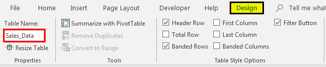
The next thing you will want to do with your table is to give it a sensible name. The table name will be used to reference the table in formulas and other tools, so giving it a short descriptive name will help you later when reading formulas.
- Go to the Table Design tab.
- Click on the Table Name input box.
- Type your new table name.
- Press the Enter key to accept the new name.
Each table in your database will need to be in a separate table, so you will need to repeat the above process for each.
How to Add New Data to Your Table
You will likely need to add new records to your database. This means you will need to add new rows to your tables.
Adding rows to an Excel table is very easy and you can do it a few different ways.
You can add new rows to your table from the right-click menu.
- Select a cell inside your table.
- Right-click on the cell.
- Select Insert from the menu.
- Select Table Rows Above from the submenu.
This will insert a new blank row directly above the selected cells in your table.
You can add a blank row to the bottom of your table with the Tab key.
- Place the active cell cursor in the lower right cell of the table.
- Press the Tab key.
A new blank row will be added to the bottom of the table.
But the easiest way to add new data to a table is to type directly below the table. Data entered directly underneath the table is automatically absorbed into the table!
Excel Workbook Layout
If you are going to create an Excel database, then you should keep it simple.
Your Excel database file should contain only the data and nothing else. This means any reports, analysis, data visualization, or other work related to the data should be done in another Excel file.
Your Excel database file should only be used for adding, editing, or deleting the data stored in the file. This will help decrease the chance of accidentally changing your data, as the only reason to open the file will be to intentionally change the data.
Each table in the database should be stored in a separate worksheet and nothing else except the table should be in that sheet. You can then name the worksheet based on the table it contains so your file is easy to navigate.
💡 Tip: Place your table starting in cell A1 and then hide the remaining columns. This way it is clear the sheet should only contain the table and nothing else.
The only other sheet you might optionally include is a table of contents to help organize the file. This is where you can list each table along with the fields it contains and a description of what these fields are.
💡 Tip: You can hyperlink the table name listed in the table of contents to its associated sheet. Select the name and press Ctrl + K to create a hyperlink. This can help you navigate the workbook when you have a lot of tables in your database.
Use Data Validation to Prevent Invalid Data
Data validation is a very important feature for any database. This allows you to ensure only specific types of data are allowed in a column.
You might create data validation rules such as.
- Only positive whole numbers are entered in a quantity column.
- Only certain product names are allowed in the product column.
- A column can’t contain any duplicate values.
- Dates are between two given dates.
Excel’s data validation tools will help you ensure the data entered in your database follow such rules.
Follow these steps to add a data validation rule to any column in your table.
- Left-click on the column heading to select the entire column.
When you hover the mouse cursor over the top of your column heading in a table, the cursor will change to a black downward pointing arrow. Left-click and the entire column will be selected.
The data validation will automatically propagate to any new rows added to the table.
- Go to the Data tab.
- Click on the Data Validation command.
This will open up the Data Validation menu where you will be able to choose from various validation settings. If there is no active validation in the cell, you should see the Any values option selected in the Allow criteria.
Only Allow Positive Whole Number Values
Follow these steps from the Data Validation menu to allow only positive whole number values to be entered.
- Go to the Settings tab in the Data Validation menu.
- Select the Whole number option from the Allow dropdown.
- Select the greater than option from the Data dropdown.
- Enter 0 in the Minimum input box.
- Press the OK button.
💡 Tip: Keep the Ignore blank option checked if you want to allow blank cells in the column.
This will apply the validation rule to the column and when a user tries to enter any number other than 1, 2, 3, etc… they will be warned the data is invalid.
Only Allow Items from a List
Selecting items from a dropdown list is a great way to avoid incorrect text input such as customer or product names.
Follow these steps from the Data Validation menu to create a dropdown list for selecting text values in a column.
- Go to the Settings tab in the Data Validation menu.
- Select the List option from the Allow dropdown.
- Check the In-cell dropdown option.
- Add the list of items to the Source input.
- Press the OK button.
📝 Note: If you place the list of possible options inside an Excel Table and select the full column for the Source reference, then the range reference will update as you add items to the table.
Now when you select a cell in the column you will see a dropdown list handle on the right of the cell. Click on this and you will be able to choose a value from a list.
Only Allow Unique Values
Suppose you want to ensure the list of products in your Products table is unique. You can use the Custom option in the validation settings to achieve this.
- Go to the Settings tab in the Data Validation menu.
- Select the Custom option from the Allow dropdown.
=(COUNTIFS(INDIRECT("Products[Item]"),A2)=1)- Enter the above formula in the Formula input.
- Press the OK button.
The formula counts the number of times the current row’s value appears in the Products[Item] column using the COUNTIFS function.
It then determines if this count is equal to 1. Only values where the formula evaluates to 1 are allowed which means the product name can’t have been in the list already.
📝 Note: You need to reference the column by name using the INDIRECT function in order for the range to grow as you add items to your table!
Show Input Message when Cell is Selected
The data validation menu allows you to show a message to your users when a cell is selected. This means you can add instructions about what types of values are allowed in the column.
Follow these steps to add an input message in the Data Validation menu.
- Go to the Input Message tab in the Data Validation menu.
- Keep the Show input message when cell is selected option checked.
- Add some text to the Title section.
- Add some text to the Input message section.
- Press the OK button.
When you select a cell in the column which contains the data validation, a small yellow pop-up will appear with your Title and Input message text.
Prevent Invalid Data with Error Message
When you have a data validation rule in place, you will usually want to prevent invalid data from being entered.
This can be achieved using the error message feature in the Data Validation menu.
- Go to the Error Alert tab in the Data Validation menu.
- Keep the Show error alert after invalid data is entered option checked.
- Select the Stop option in the Style dropdown.
- Add some text to the Title section.
- Add some text to the Error message section.
- Press the OK button.
📝 Note: The Stop option is essential if you want to prevent the invalid data from being entered rather than only warning the user the data is invalid.
When you try to enter a repeated value in the column your custom error message will pop up and prevent the value from being entered in the cell.
Data Entry Form for Your Excel Database
Excel doesn’t have any fool-proof methods to ensure data is entered correctly, even when data validation techniques previously mentioned are used.
When a user copies and pastes or cuts and pastes values, this can override data validation in a column and cause incorrect data to enter into your database.
Using a data entry form can help to avoid data entry errors and there are a couple of different options available.
- Use a table for data entry.
- Use the quick access toolbar data entry form.
- Use Microsoft Forms for data entry.
- Use Microsoft Power Automate app for data entry.
- Use Microsoft Power Apps for data entry.
💡 Tip: Check out this post for more details on the various data entry form options for Excel.
Tools such as Microsoft Forms, Power Automate, and Power Apps will give you more data validation, access, and security controls over your data entry compared with the basic Excel options.
Access and Security for Your Excel Database
Excel isn’t a secure option for your data.
Whatever measures you set up in your Excel file to prevent users from changing data by accident or on purpose will not be foolproof.
Whoever has access to the file will be able to create, read, update, and delete data from your database if they are determined. There are also no options to assign certain privileges to certain users within an Excel file.
However, you can manage access and security to the file from SharePoint.
💡 Tip: Check out this post from Microsoft about recommendations for securing SharePoint files for more details.
When you store your Excel file in SharePoint you’ll also be able to see recent changes.
- Go to the Review tab.
- Click on the Show Changes command.
This will open up the Changes pane on the right-hand side of the Excel sheet.
It will show you a chronological list of all the recent changes in the workbook, who made those changes, when they made the change, and what the previous value was.
You can also right-click on a cell and select Show Changes. This will open the Changes pane filtered to only show the changes for that particular cell.
This is a great way to track down the cause of any potential errors in your data.
Query Your Excel Database with Power Query
Your Excel database file should only be used to add, edit, or delete records in your tables.
So how do you use the data for anything else such as creating reports, analysis, or dashboards?
This is the magic of Power Query! It will allow you to connect to your Excel database and query the data in a read-only manner. You can build all your reports, analysis, and dashboards in a separate file which can easily be refreshed with the latest data from your Excel database file.
Here’s how to use power query to quickly import your data into any Excel file.
- Go to the Data tab.
- Click on the Get Data command.
- Choose the From File option.
- Choose the From Excel Workbook option in the submenu.
This will open a file picker menu where you can navigate to your Excel database file.
- Select your Excel database file.
- Click on the Import button.
⚠️ Warning: Make sure your Excel database file is closed or the import process will show a warning that it’s unable to connect to the file because it’s in use!
Clicking on the Import button will then open the Navigator menu. This is where you can select what data to load and where to load it.
The Navigator menu will list all the tables and sheets in the Excel file. Your tables might be listed with a suffix on the name if you’ve named the sheets and tables the same.
- Check the option to Select multiple items if you want to load more than one table from your database.
- Select which tables to load.
- Click on the small arrow icon next to the Load button.
- Select the Load To option in the Load submenu.
This will open the Import Data menu where you can choose to import your data into a Table, PivotTable, PivotChart, or only create a Connection to the data without loading it.
- Select the Table option.
- Click on the OK button.
Your data is then loaded into an Excel Table in the new workbook.
The best part is you can always get the latest data from the source database file. Go to the Data tab and press the Refresh All button to refresh the power query connection and import the latest data.
💡 Tip: You can do a lot more than just load data with Power Query. You can also transform your data in just about any imaginable way using the Transform Data button in the Navigator menu. Check out this post on how to use Power Query for more details about this amazing tool.
Analyze and Summarize Your Excel Database with Power Pivot
Power Query isn’t the only database tool Excel has. The data model and Power Pivot add-in will help you slice and dice relational data inside your Excel pivot tables.
When you load your data with Power Quer, there is an option to Add this data to the Data Model in the Import Data menu.
This option will allow you to build relationships between the various tables in your database. This way you’ll be able to analyze your orders by category even though this field doesn’t appear in the Orders table.
You can build your table relationships from the Data tab.
- Go to the Data tab.
- Click on either the Relationships or Manage Data Model command.
Now you’ll be able to analyze multiple tables from your database inside a single pivot table!
Conclusions
Data is an essential part of any business or organization. If you need to track customers, sales, inventory, or any other information then you need a database.
If you need to create a database on a budget with the tools you have available then Microsoft Excel might be the best option and is a natural fit for any tabular data because of its row and column structure.
There are many things to consider when using Excel as a database such as who will have access to the files, what type of data will be stored, and how you will use the data.
Features such as Tables, data validation, power query, and power pivot are all essential to properly storing, managing, and accessing your data.
Do you use Excel as a database? Do you have any other tips for using Excel to manage your dataset? Let me know in the comments below!
About the Author
John is a Microsoft MVP and qualified actuary with over 15 years of experience. He has worked in a variety of industries, including insurance, ad tech, and most recently Power Platform consulting. He is a keen problem solver and has a passion for using technology to make businesses more efficient.
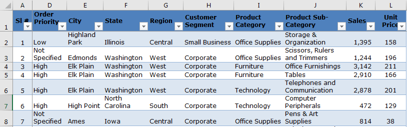
Excel is a combination of rows and columns, and these rows and columns store our data, which in other terms are named records. As Excel is the most common tool, we reserve the data in Excel, making it a database. Therefore, when we put data in Excel in some form of tables in rows and columns and give the table a name, that is a database in Excel. We can also import data from other sources in Excel, given the data format is proper with the Excel format.
For example, you may create a company’s sales report of different regions on a database in Excel for easy access and complete control over data management while working with the program.
Creating an Excel Database
Having the data in Excel will make life easier for you because Excel is a powerful tool where we can play with the data. If you maintain the data in other sources, you may not correctly get all the formulas, dates, and time format. I hope you have experienced this in your daily work. Having the data in the right database platform is very important. Having the data in Excel has its pros and cons. However, if you are a regular user of Excel, it is much easier to work with Excel. This article will show you how to create a database in Excel.
Table of contents
- Creating an Excel Database
- How to Create a Database in Excel?
- Things to Remember While Creating a Database in Excel
- Recommended Articles
How to Create a Database in Excel?
We do not see any of the schools are colleges teaching us to Excel as the software in our academics. Whatever business models, we learn a theory until joining the corporate company.
The biggest problem with this theoretical knowledge is it does not support real-time life examples. But, nothing to worry about; we will guide you through the process of creating a database in Excel.
We need to design the Excel worksheet carefully to have accurate data in the database format.
You can download this Create Database Excel Template here – Create Database Excel Template
Follow the below steps to create a database in Excel.
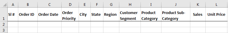
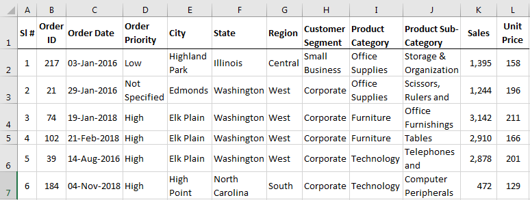
- We must first ensure all the required columns and name each heading properly.

- Once the headers of the data table are clear, we can easily start entering the data just below the respective column headings.

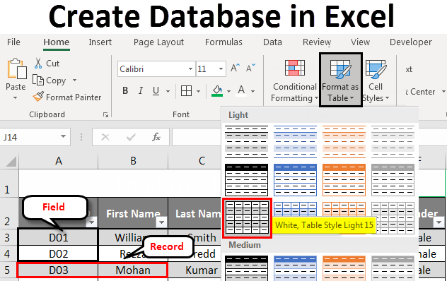
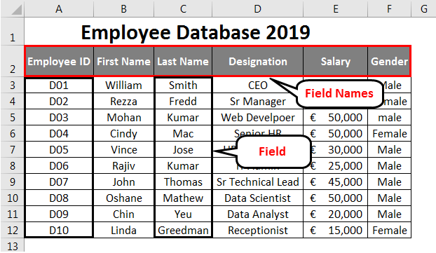
In database terminology, rows are called Records, and columns are called Fields.
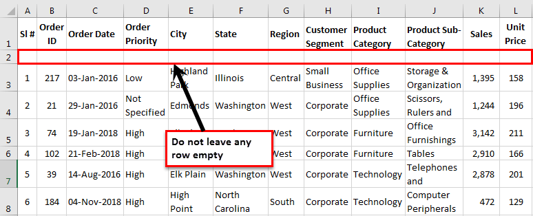
- We cannot leave a single row empty when entering the data. For example, we have entered the headings in the first row, and if we start entering the data from the third row by leaving the 2nd row empty, we are gone.

Not only the first or second row, but we also cannot leave any row empty after entering certain data into the database field.
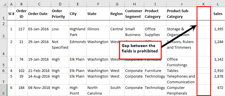
- As we said, each column is called Fields in the database. Similarly, we cannot have an empty field between the data.
We need to enter the fields one after the other. Having a gap of even one column or field is strictly prohibited.

I am so stressed about not having an empty record or field because when the data needs to be exported to other software or the web, as soon as the software sees the blank record or field, it assumes that it is the end of the data. Therefore, it may not consider the full data.
- We must fill in all the data carefully.
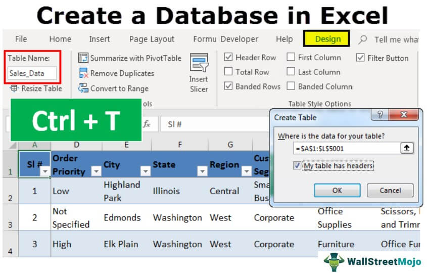
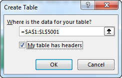
In the above image, I have data all the way from row 1 to row 5001. - The final thing we need to do is convert this data to an excel table. By selecting the data, press Ctrl + T.

- Here, we need to make sure the My table has a header checkbox is ticked and the range is selected properly.

- Then, we must click on OK to complete the table creation. As a result, we may have a table like this now.

- We must now give a proper name to the table under the table Design tab.

- Since we have created a table, automatically, it would expand whenever we enter the data after the last column.
We have the database ready now. Follow the pros and cons below to have a good hand on your database.

Things to Remember While Creating a Database in Excel
- We can upload the file to MS Access to have a secure database and back up a platform.
- Since we have all the data in Excel, it is very easy for your calculations and statistics.
- Excel is the best tool for database analysis.
- Easy to read and not complicated because of clear fields and records.
- We can filter out the records by using auto filters.
- If possible, sort the data according to date-wise.
- As the data keeps growing, Excel will slow down considerably.
- We cannot share more than 34 MB files with others in an email.
- We can Apply the Pivot tableA Pivot Table is an Excel tool that allows you to extract data in a preferred format (dashboard/reports) from large data sets contained within a worksheet. It can summarize, sort, group, and reorganize data, as well as execute other complex calculations on it.read more and give a detailed analysis of the database.
- We can download the workbook and use it for your practice purpose.
Recommended Articles
This article is a guide to Databases in Excel. Here, we discuss creating a database in Excel with examples and downloadable Excel templates. You may also look at these useful functions in Excel: –
- Excel Database Template
- Match Data using Excel Functions
- Forms for Data Entry in Excel
- Create a Data Table in Excel
- SUMIFS with Dates
Excel Create Database (Table of Contents)
- Create a Database in Excel
- How to Create a Database in Excel?
Introduction to Create Database in Excel
If you want to create a database, MS Access is the tool you ideally should look for. However, it is a bit complicated to learn and master the techniques therein as MS Access. It would help if you had ample time to master those. In such cases, you can use excel as a good resource to create a database. It is easier to enter, store, and find specific information in the Excel Database. A well-structured, well-formatted excel table can be considered as a database itself. So, all you have to do is create a table that has a proper format. If the table is well-structured, you can sort the data in many different ways. Moreover, you can apply the filters to well-structured data to slice and dice it as per your requirements.
How to Create a Database in Excel?
We’ll be creating an employee database for the organization. Let’s see how to create a database in Excel by following the below process:
You can download this Create Database Excel Template here – Create Database Excel Template
Data Entering to Create Excel Database
Data entering is the main aspect while you are trying to create a database in Excel.
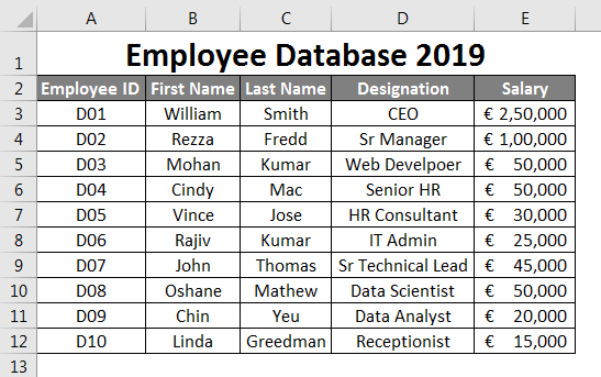
Suppose this is the data thatq1 you are going to use as an employee database.
I have added the first few Employee ID’s. Say D01, D02, D03 and then dragged the remaining till row 12 using Fill Handle. Column second onwards contains the general employee information like First Name, Last Name, Designation, and Salary. Filthis informationon in cells manually as per your details. Make sure the Salary column format is applied to all the cells in the column (Otherwise, this database may cause an error while using).
Entering Correct Data
It is always good to enter the correct data. Make sure there is no space in your data. When I say no other blanks, it covers the column cells, which are not blank as well. Try to the utmost that no data cells are blank. If you don’t have any information available with you, prefer to put NA over a blank cell. It’s also important to make the right input to the right column.
See the screenshot below:
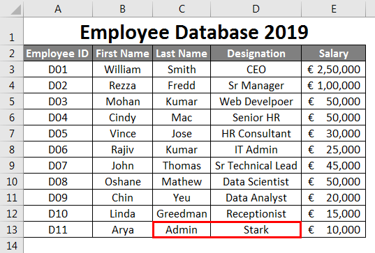
Suppose,uy as shown in the image above, you wrongly interchanged the column inputs. i.e. you have mentioned Designation under Last Name and Last Name under Designation, which is a serious drop-back when you are thinking of this as a master employee data for your organization. It may mislead some of your conclusions.
Suppose you have added a correct entry, but at the 2nd row after the last row (i.e. one row is left blank). It is also not recommended to do so. It is a breakdown for your data. See screenshot given below:
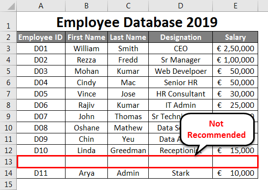
As you can see, there is one row left blank after row no. 12 ( second last row of the dataset) and added one new row, which is not recommended. On similar lines, you should not leave any blank column in the database.
Let’s see the screenshot below:
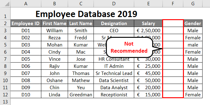
As you can see, column F is left blank. Which causes Excel to think there is a split of data. Excel considers that a blank column is a separator for two databases. It is misleading, as the column after the blank column is a part of your original database. It’s not the start column of a new database.
All the Rows are called Record in Excel Database.
It is a kind of basic knowledge we should have about the database we are creating. Every single row we create/add is called as a Record in the database. See the below screenshot for your reference:
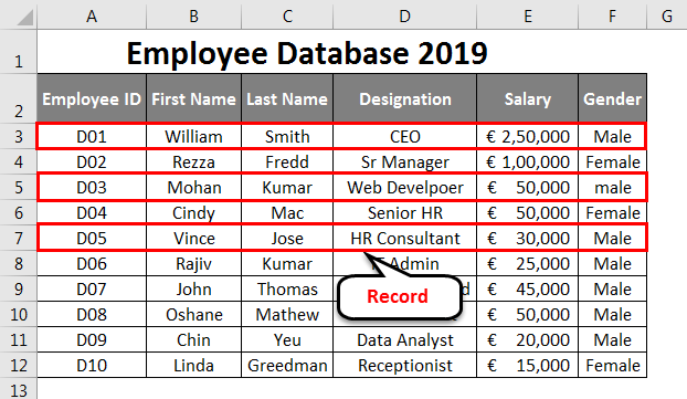
Every Column is a Field in Excel Database
Every column is called Field in the Excel database. The column headings are called Field Names.
Format Table
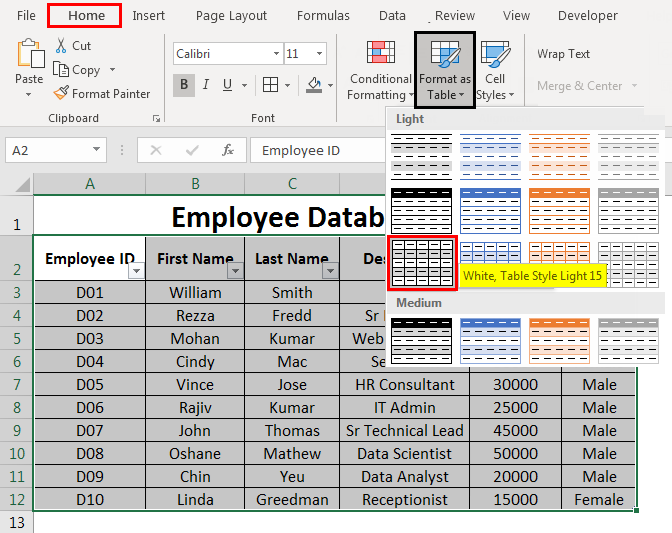
Once you are done with inputting the data, it should be converted into a better visualisation table.
- Select cells A2 to F12 from the spreadsheet.
- Go to the Home tab.
- Select Format as Table drop-down menu. You can choose a table layout of your own.
Once you click a particular table format, a table window will pop up with the range of data selected, and a dotted line will surround that range. You can change the range of the data therein in the table dialog box as well.
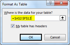
Once you are happy with the range, you can choose, OK. You can see your data in a tabular form now. See the screenshot given below:
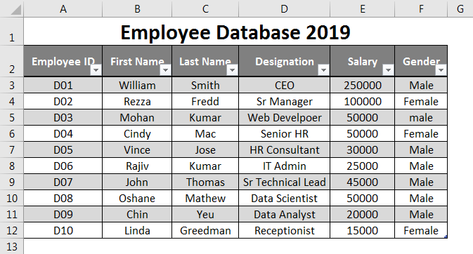
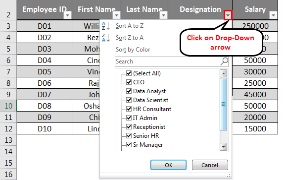
Use Excel Database Tools to Sort or Filter the Data
You can use the drop-down arrows situated beside each Field Name to Sort or Filter the data as per your requirement. These options are really helpful when you are dealing with a large amount of data.
Expanding the Database
If you want to add some more records to your table, you can do it as well. Select all the cells from your table.
Place your mouse at the bottom of the last cell of your table. The mouse pointer will turn into a two-headed arrow. You can drag down the pointer from there until you want to add that many blank rows in your database. Subsequently, you can add data under those blank cells as well.
Database Formatting
Highlight cell A1 to F1 from the spreadsheet.
- Select Home tab
- Under the Home tab, go to Wrap Text as well as Merge and Center.
- You can also change the fill colour. Select Fill Color. Choose the colour of your interest. Here I have selected Green as a colour.
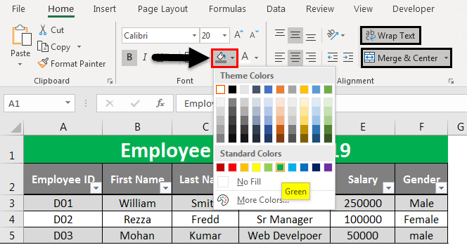
This is how we have created our Database in Excel.
Things to Remember About Create Database in Excel
- Information about one item should be populated in one single row entirely. You can’t use multiple lines to add different data of the same item in the excel database.
- The field should not be kept empty. (Including Column Headings/Field Name).
- The data type entered in one column should be homogeneous. For, e.g. If you are entering Salary details in the Salary column, there should not be any text string in that column. Similarly, any column containing text strings should not contain any numerical information.
- The database created here is really a very small example. It becomes huge in terms of employees joining every now and then and becomes hectic to maintain the data again and again with the standard formatting. That’s why it is recommended to use databases.
Recommended Articles
This has been a guide to Create a Database in Excel. Here we discuss how to Create a Database in Excel along with practical examples and a downloadable excel template. You can also go through our other suggested articles –
- Excel Import Data
- Table styles in Excel
- Toolbar in Excel
- Excel Rows and Columns