
Excel for Microsoft 365 Excel 2021 Excel 2019 Excel 2016 Excel 2013 Excel 2010 Excel 2007 Excel Starter 2010 More…Less
You can quickly create a named range by using a selection of cells in the worksheet.
Note: Named ranges that are created from selecting cells have a workbook-level scope.
-
Select the range you want to name, including the row or column labels.
-
Click Formulas > Create from Selection.
-
In the Create Names from Selection dialog box, select the checkbox (es) depending on the location of your row/column header. If you have only a header row at the top of the table, then just select Top row. Suppose you have a top row and left column header, then select Top row and Left column options, and so on.
-
Click OK.
Need more help?
You can always ask an expert in the Excel Tech Community or get support in the Answers community.
Need more help?
Home / Excel Formulas / Create a Date Range in Excel
While working in data where you have dates, you might have to create a range of dates. A range is something that has a start date and an end date. In this tutorial, you will learn to create a date range.
Create a Date Range Starting from Today
Now let’s say you want to create a date range of seven days starting from today. In the following example, we have today’s date in cell A1 which we have got by using today’s function.

=A1+7To create a date range, follow these simple steps:
- Enter the “=” in cell B1, or any other cell.
- Refer to cell A1, where you have the starting date of the range.
- Use the “+” sign to add days to today’s date.
- Specify the number of days you want to add to today’s date.

Create a Date Range in a Single Cell
Let’s go a little further and create a date range in a single cell. And for this, we need to combine both starting date and the ending date in a single cell. But the problem is when you try to combine two dates within a single cell it returns something like the below.

Now to overcome this problem we need to use the TEXT function to convert dates into text and then combine them as a range of dates. The formula would be something like the one below.

=TEXT(A1,"dd/mmm/yy")&" --- "&TEXT(B1,"dd/mmm/yy")Now as you can see, we have a range of dates in cell C1 starting from 8-Feb-22 to 15-Feb-22. And if you want to create a range of dates in a single cell, you can use the following formula.
=TEXT(TODAY(),"dd/mmm/yy")&" --- "&TEXT(A1+7,"dd/mmm/yy")In the part about using the TEXT function, you can change the format of the date the way you want.
Download Sample File
- Ready
sample-file
Date Range in Excel Formula
We need to perform different operations like addition or subtraction on date values with Excel. By setting date ranges in Excel, we can perform calculations on these dates. For setting date ranges in Excel, we can first format the cells that have a start and end date as ‘Date’ and then use the operators: ‘+’ or ‘-‘to determine the end date or range duration.
For example, suppose we have two dates in cells A2 and B2. To create a date range, we may use the following formula with the TEXT function:
=TEXT(A2,”mm/dd”)&” – “&TEXT(B2,”mm/dd”)
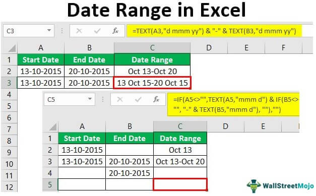
Table of contents
- Date Range in Excel Formula
- Examples of Date Range in Excel
- Example #1 – Basic Date Ranges
- Example #2 – Creating Date Sequence
- Example #3
- Example #4
- Things to Remember
- Recommended Articles
- Examples of Date Range in Excel
Examples of Date Range in Excel
You can download this Date Range Excel Template here – Date Range Excel Template
Example #1 – Basic Date Ranges
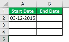
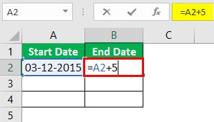
Let us see how adding a number to a date can create a date range.
Suppose we have a start date in cell A2.
If we add a number, say 5, to it, we can build a date range.
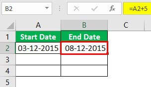
When we select cell A3 and type “=B2 + 1.”
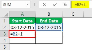
Then, we need to copy cell B2 and paste it into cell B3; the relative cell referenceCell reference in excel is referring the other cells to a cell to use its values or properties. For instance, if we have data in cell A2 and want to use that in cell A1, use =A2 in cell A1, and this will copy the A2 value in A1.read more would change as follows:
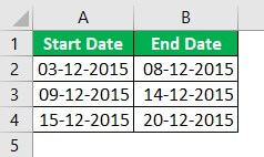
So we can see that multiple date ranges can be built this way.
Example #2 – Creating Date Sequence
With Excel, we can easily create several sequences. Now we know that dates are some numbers in Excel. So we can use the same method to generate date ranges. So to create date ranges that have the same range or gap, but the dates change as we go down, we can follow the below steps:
- We must first type a start date and end date in a minimum of two rows.
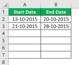
- Then, select the ranges and drag them down below the row where we require the dates ranges.
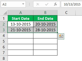
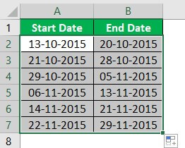
So we can see that using the date ranges in the first two rows as a template, Excel automatically creates date ranges for the subsequent rows.
Example #3
Now, suppose we have two dates in two cells, and we wish to display them concatenated as a date range in a single cell. For doing this, we can use a formula based on the ‘TEXT’ function can be used. The general syntax for this formula is as follows:
= TEXT(date1,”format”) & ” – ” & TEXT(date2,”format”)
Case 1:
This function receives two date values as numeric and concatenates these two dates in the form of a date range according to a custom date format (“mmm d” in this case):
Date Range =TEXT(A2,”mmm d”) & “-” & TEXT(B2,”mmm d”)
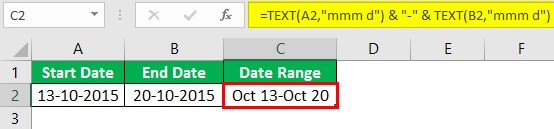
So we can see in the above screenshot that we have applied the formula in cell C2. The TEXT function receives the dates stored in cells A2 and B2. The ampersand ‘&’ operator is used to concatenate the two dates as a date range in a custom format, specified as “mmm d” in this case, in a single cell, and the two dates are joined with a hyphen ‘-‘ in the resultant date range which is determined in cell C2.
Case 2:
In this example, we wish to combine the two dates as a date range in a single cell with a different format, say “d mmm yy.” So the formula for a date range, in this case, would be as follows:
Date Range =TEXT(A3,”d mmm yy”) & “-” & TEXT(B3,”d mmm yy”)
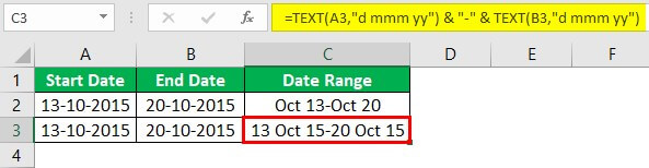
So we can see in the above screenshot that the TEXT function receives the dates stored in cells A3 and B3, and the ampersand ‘&’ operator is used to concatenate the two dates as a date range in a custom format, specified as “d mmm yy” in this case, in a single cell. Then, finally, the two dates are joined with a hyphen ‘-‘in the resultant date range determined in cell C3.
Example #4
Now let us see what happens if the start date or end date is missing. For example, suppose the end date is missing as follows:
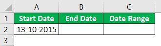
The formula based on the TEXT function that we have used above would not work correctly if the end date is missing. As the hyphen in the formula would anyhow be appended to the start date, i.e., along with the start date, we would also see a hyphen displayed in the date range. In contrast, we would only wish to see the start date as the date range if the end date is missing.
So, in this case, we can have the formula by wrapping the concatenation and the second TEXT function inside an IF clause as follows:
Date Range =TEXT(A2,”mmm d”) & IF(B2<> “”, “-” & TEXT(B2,”mmm d”), “”)
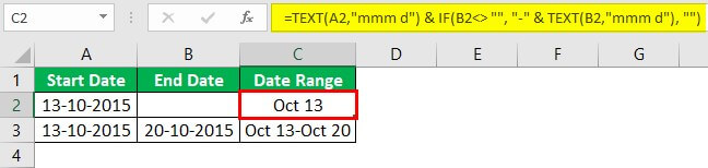
So we can see that the above formula creates a full date range using both the dates when both are present. However, it displays only the start date in the specified format if the end date is missing. It is done with the help of an IF clause.
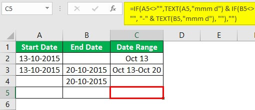
Now in case both the dates are missing, we could use a nested IF statement in excelIn Excel, nested if function means using another logical or conditional function with the if function to test multiple conditions. For example, if there are two conditions to be tested, we can use the logical functions AND or OR depending on the situation, or we can use the other conditional functions to test even more ifs inside a single if.read more, (i.e., one IF inside another IF statement) as follows:
Date Range =IF(A4<>””,TEXT(A4,”mmm d”) & IF(B4<> “”, “-” & TEXT(B4,”mmm d”), “”),””)

So we can see that the above formula returns an empty string if the start date is missing.
If both the dates are missing, an empty string is also returned.
Things to Remember
- We can even create a list of sequential dates using the ‘Fill Handle’ command. We can select the cell having a start date and then drag it to the range of cells where we wish to fill. Next, click on the “Home” tab -> “Editing” ->”Fill Series” and then choose a date unit we want to use.
- If we wish to calculate the duration or number of days between two dates, we can subtract the two dates using the ‘-‘operator, and we will get the desired result.

Note: The format of cells: A2 and B2 is ‘Date,’ whereas that of cell C2 is ‘General’ as it calculates the number of days.
Recommended Articles
This article has been a guide to Date Range in Excel. Here, we discuss formulas to create date ranges in Excel in different ways and a downloadable Excel template. You may learn more about Excel from the following articles: –
- DATE Excel Function
- EDATE Excel Function
- Subtract Date In Excel
- Compare Dates in Excel
What’s in the name?
If you are working with Excel spreadsheets, it could mean a lot of time saving and efficiency.
In this tutorial, you’ll learn how to create Named Ranges in Excel and how to use it to save time.
Named Ranges in Excel – An Introduction
If someone has to call me or refer to me, they will use my name (instead of saying a male is staying in so and so place with so and so height and weight).
Right?
Similarly, in Excel, you can give a name to a cell or a range of cells.
Now, instead of using the cell reference (such as A1 or A1:A10), you can simply use the name that you assigned to it.
For example, suppose you have a data set as shown below:
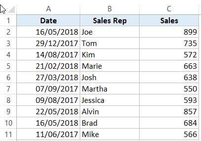
In this data set, if you have to refer to the range that has the Date, you will have to use A2:A11 in formulas. Similarly, for Sales Rep and Sales, you will have to use B2:B11 and C2:C11.
While it’s alright when you only have a couple of data points, but in case you huge complex data sets, using cell references to refer to data could be time-consuming.
Excel Named Ranges makes it easy to refer to data sets in Excel.
You can create a named range in Excel for each data category, and then use that name instead of the cell references. For example, dates can be named ‘Date’, Sales Rep data can be named ‘SalesRep’ and sales data can be named ‘Sales’.

You can also create a name for a single cell. For example, if you have the sales commission percentage in a cell, you can name that cell as ‘Commission’.
Benefits of Creating Named Ranges in Excel
Here are the benefits of using named ranges in Excel.
Use Names instead of Cell References
When you create Named Ranges in Excel, you can use these names instead of the cell references.
For example, you can use =SUM(SALES) instead of =SUM(C2:C11) for the above data set.
Have a look at ṭhe formulas listed below. Instead of using cell references, I have used the Named Ranges.
- Number of sales with value more than 500: =COUNTIF(Sales,”>500″)
- Sum of all the sales done by Tom: =SUMIF(SalesRep,”Tom”,Sales)
- Commission earned by Joe (sales by Joe multiplied by commission percentage):
=SUMIF(SalesRep,”Joe”,Sales)*Commission
You would agree that these formulas are easy to create and easy to understand (especially when you share it with someone else or revisit it yourself.
No Need to Go Back to the Dataset to Select Cells
Another significant benefit of using Named Ranges in Excel is that you don’t need to go back and select the cell ranges.
You can just type a couple of alphabets of that named range and Excel will show the matching named ranges (as shown below):

Named Ranges Make Formulas Dynamic
By using Named Ranges in Excel, you can make Excel formulas dynamic.
For example, in the case of sales commission, instead of using the value 2.5%, you can use the Named Range.
Now, if your company later decides to increase the commission to 3%, you can simply update the Named Range, and all the calculation would automatically update to reflect the new commission.
How to Create Named Ranges in Excel
Here are three ways to create Named Ranges in Excel:
Method #1 – Using Define Name
Here are the steps to create Named Ranges in Excel using Define Name:
This will create a Named Range SALESREP.
Method #2: Using the Name Box
- Select the range for which you want to create a name (do not select headers).
- Go to the Name Box on the left of Formula bar and Type the name of the with which you want to create the Named Range.

- Note that the Name created here will be available for the entire Workbook. If you wish to restrict it to a worksheet, use Method 1.
Method #3: Using Create From Selection Option
This is the recommended way when you have data in tabular form, and you want to create named range for each column/row.
For example, in the dataset below, if you want to quickly create three named ranges (Date, Sales_Rep, and Sales), then you can use the method shown below.
Here are the steps to quickly create named ranges from a dataset:
This will create three Named Ranges – Date, Sales_Rep, and Sales.
Note that it automatically picks up names from the headers. If there are any space between words, it inserts an underscore (as you can’t have spaces in named ranges).
Naming Convention for Named Ranges in Excel
There are certain naming rules you need to know while creating Named Ranges in Excel:
- The first character of a Named Range should be a letter and underscore character(_), or a backslash(). If it’s anything else, it will show an error. The remaining characters can be letters, numbers, special characters, period, or underscore.
- You can not use names that also represent cell references in Excel. For example, you can’t use AB1 as it is also a cell reference.
- You can’t use spaces while creating named ranges. For example, you can’t have Sales Rep as a named range. If you want to combine two words and create a Named Range, use an underscore, period or uppercase characters to create it. For example, you can have Sales_Rep, SalesRep, or SalesRep.
- While creating named ranges, Excel treats uppercase and lowercase the same way. For example, if you create a named range SALES, then you will not be able to create another named range such as ‘sales’ or ‘Sales’.
- A Named Range can be up to 255 characters long.
Too Many Named Ranges in Excel? Don’t Worry
Sometimes in large data sets and complex models, you may end up creating a lot of Named Ranges in Excel.
What if you don’t remember the name of the Named Range you created?
Don’t worry – here are some useful tips.
Getting the Names of All the Named Ranges
Here are the steps to get a list of all the named ranges you created:
This will give you a list of all the Named Ranges in that workbook. To use a named range (in formulas or a cell), double click on it.

Displaying the Matching Named Ranges
- If you have some idea about the Name, type a few initial characters, and Excel will show a drop down of the matching names.


How to Edit Named Ranges in Excel
If you have already created a Named Range, you can edit it using the following steps:
Useful Named Range Shortcuts (the Power of F3)
Here are some useful keyboard shortcuts that will come handy when you are working with Named Ranges in Excel:
- To get a list of all the Named Ranges and pasting it in Formula: F3
- To create new name using Name Manager Dialogue Box: Control + F3
- To create Named Ranges from Selection: Control + Shift + F3
Creating Dynamic Named Ranges in Excel
So far in this tutorial, we have created static Named Ranges.
This means that these Named Ranges would always refer to the same dataset.
For example, if A1:A10 has been named as ‘Sales’, it would always refer to A1:A10.
If you add more sales data, then you would have to manually go and update the reference in the named range.
In the world of ever-expanding data sets, this may end up taking up a lot of your time. Every time you get new data, you may have to update the Named Ranges in Excel.
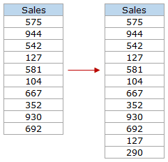
To tackle this issue, we can create Dynamic Named Ranges in Excel that would automatically account for additional data and include it in the existing Named Range.
For example, For example, if I add two additional sales data points, a dynamic named range would automatically refer to A1:A12.
This kind of Dynamic Named Range can be created by using Excel INDEX function. Instead of specifying the cell references while creating the Named Range, we specify the formula. The formula automatically updated when the data is added or deleted.
Let’s see how to create Dynamic Named Ranges in Excel.
Suppose we have the sales data in cell A2:A11.

Here are the steps to create Dynamic Named Ranges in Excel:
-
- Go to the Formula tab and click on Define Name.

- In the New Name dialogue box type the following:
- Name: Sales
- Scope: Workbook
- Refers to: =$A$2:INDEX($A$2:$A$100,COUNTIF($A$2:$A$100,”<>”&””))

- Click OK.
- Go to the Formula tab and click on Define Name.


Done!
You now have a dynamic named range with the name ‘Sales’. This would automatically update whenever you add data to it or remove data from it.
How does Dynamic Named Ranges Work?
To explain how this work, you need to know a bit more about Excel INDEX function.
Most people use INDEX to return a value from a list based on the row and column number.
But the INDEX function also has another side to it.
It can be used to return a cell reference when it is used as a part of a cell reference.
For example, here is the formula that we have used to create a dynamic named range:
=$A$2:INDEX($A$2:$A$100,COUNTIF($A$2:$A$100,"<>"&""))
INDEX($A$2:$A$100,COUNTIF($A$2:$A$100,”<>”&””) –> This part of the formula is expected to return a value (which would be the 10th value from the list, considering there are ten items).
However, when used in front of a reference (=$A$2:INDEX($A$2:$A$100,COUNTIF($A$2:$A$100,”<>”&””))) it returns the reference to the cell instead of the value.
Hence, here it returns =$A$2:$A$11
If we add two additional values to the sales column, it would then return =$A$2:$A$13
When you add new data to the list, Excel COUNTIF function returns the number of non-blank cells in the data. This number is used by the INDEX function to fetch the cell reference of the last item in the list.
Note:
- This would only work if there are no blank cells in the data.
- In the example taken above, I have assigned a large number of cells (A2:A100) for the Named Range formula. You can adjust this based on your data set.
You can also use OFFSET function to create a Dynamic Named Ranges in Excel, however, since OFFSET function is volatile, it may lead a slow Excel workbook. INDEX, on the other hand, is semi-volatile, which makes it a better choice to create Dynamic Named Ranges in Excel.
You may also like the following Excel resources:
- Free Excel Templates.
- Free Online Excel Training (7-Part Online Video Course).
- Useful Excel Macro Code Examples.
- 10 Advanced Excel VLOOKUP Examples.
- Creating a Drop Down List in Excel.
- Creating a Named Range in Google Sheets.
- How to Reference Another Sheet or Workbook in Excel
- How to Delete Named Range in Excel?
Author: Oscar Cronquist Article last updated on February 25, 2019
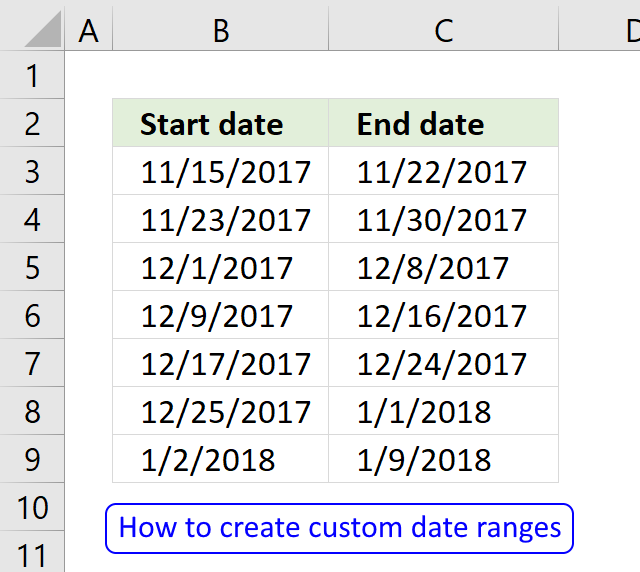
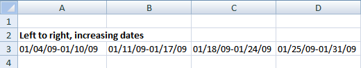
Question: I am trying to create an excel spreadsheet that has a date range. Example:
Cell A1 1/4/2009-1/10/2009
Cell B1 1/11/2009-1/17/2009
Cell C1 1/18/2009-1/24/2009
How do I create a formula to do this?
I will in this article discuss what Excel dates actually are, how to use them in formulas and how to create a sequence of dates that you can use as date ranges.
What is on this page?
- Explaining Excel dates
- Basic date ranges
- Create a date sequence
- Advanced formula
- Explaining advanced formula
- Get workbook
What are dates in Excel?
First, what are dates in Excel? They are actually numbers and I will prove it to you, try these steps:
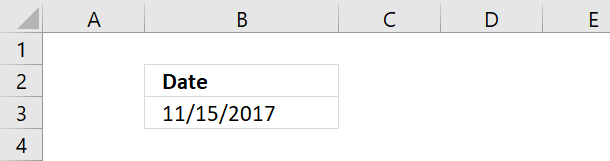
- Type a date in a cell
- Select the cell
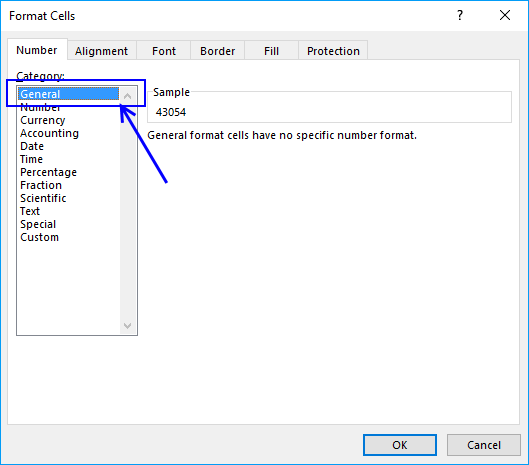
- Press CTRL + 1 to open the «Format Cells» dialog box
- Select «General»

- Press with left mouse button on OK button
- The cell you selected now has a different formatting. This shows you what dates are in Excel.
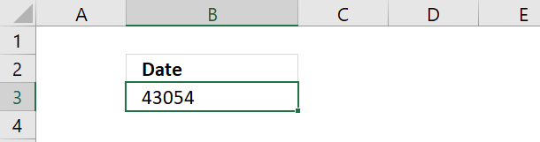
Date 11/15/2017 is 43054. Excel starts numbering dates at 1/1/1900 with value 1. Type 1 in a cell and change the cell formatting to «Date» and see what Excel displays.
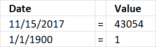
Date 11/15/2017 is 43053 days from 1/1/1900. This means also that you can’t use dates prior to 1/1/1900.
Recommended articles
- How to format date values
- Calculate last date in month
- Find latest date based on a condition
- Workdays within date range
Back to top
Basic date ranges
You can build a formula or use a built-in feature to build date ranges, read on to learn more.
Now you know that dates in Excel are numbers. You can easily create a date range by adding a number to a date.
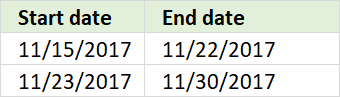
The picture below shows a start date 11/15/2017, adding number 7 to that date returns 11/22/2017
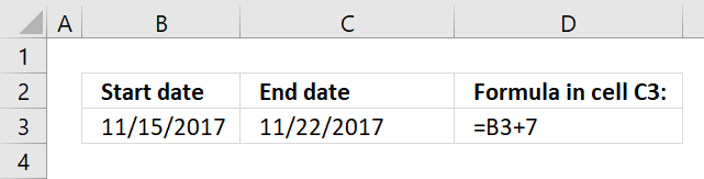
This allows you to quickly build date ranges simply by adding a number to a date.
Now select cell B4 and type =C3+1
Copy cell C3 and paste to cell C4.
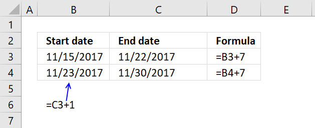
Relative cell references changes when you copy a cell and paste it to a new cell and I am going to use that now.
Copy cell range B4:C4 and paste it to cells below.
You have now built multiple date ranges using simple mathematics.
Create a date sequence
Excel has a great built-in feature that allows you to create number sequences in no time. Since dates are numbers in Excel you can use the same technique to build date ranges.
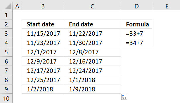
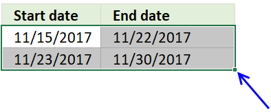
To build date ranges that have the same range but dates change, follow these steps:
- Type the start date and the end date in a cell each
- Type the second start date an end date in cells below

- Select both date ranges
- Press and hold on black dot

- Drag to cells below

- Release mouse button

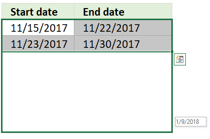
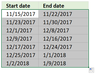
Excel has now built date ranges automatically using the two first date ranges as a template.
Recommended articles
- Use MEDIAN function to calculate overlapping ranges
- Identify overlapping date ranges
- Count overlapping days across multiple date ranges
- Find missing dates in a set of date ranges
- Category: Overlapping date ranges
Back to top
Advanced formula

If you need to build date ranges that have both the start and end date in the same cell you need to build a more complicated formula. The TEXT function lets you format dates out of numbers.
See row 3 in the above picture.
Date ranges horizontally
The following formula returns date ranges that exists after the start date, the start date in this case is 1/4/2009, however you can easily change that.
The DATE function creates the number using three arguments. The first argument is the year, the second argument is the month and the third argument is the day.
DATE(year, month, day)
Formula in cell A3:
=TEXT(DATE(2009, 1, 4)+(COLUMNS($A:A)-1)*7, «mm/dd/yy»)&»-«&TEXT(DATE(2009, 1, 4)+(COLUMNS($A:A)-1)*7+6, «mm/dd/yy»)
Copy cell A3 and paste to cells to the right as far as needed.
This formula returns date ranges that are prior to the given start date.
Formula in A6:
=TEXT(DATE(2009,1,4)+(2-COLUMN(A:A)-1)*7,»mm/dd/yy»)&»-«&TEXT(DATE(2009,1,4)+(2-COLUMN(A:A)-1)*7+6,»mm/dd/yy»)
Date ranges vertically
Formula in A9:
=TEXT(DATE(2009, 1, 4)+(ROW(1:1)-1)*7, «mm/dd/yy»)&»-«&TEXT(DATE(2009, 1, 4)+(ROW(1:1)-1)*7+6, «mm/dd/yy»)
Formula in A18:
=TEXT(DATE(2009, 1, 4)+(2-ROW(1:1)-1)*7, «mm/dd/yy»)&»-«&TEXT(DATE(2009, 1, 4)+(2-ROW(1:1)-1)*7+6, «mm/dd/yy»)
Back to top
How the formula in cell A3 works
The goal with the formula above is to create a date range from Sunday to Saturday. When cell A3 is copied and pasted to the right, the date range adjusts accordingly.
The formula consists of two parts. The first part calculates the start date of the date range. I have bolded the start date part of the formula below.
=TEXT(DATE(2009, 1, 4)+(COLUMNS($A:A)-1)*7, «mm/dd/yy»)&»-«&TEXT(DATE(2009, 1, 4)+(COLUMNS($A:A)-1)*7+6, «mm/dd/yy»)
Step 1 — First part of the formula creates the start date (bolded)
I have bolded the start date in this date range: 01/04/09 — 01/10/09.
TEXT(DATE(2009, 1, 4)+(COLUMNS($A:A)-1)*7, «mm/dd/yy»)
DATE(2009, 1, 4) is the start date of the date range series.
DATE(2009, 1, 4) returns 39817
(COLUMN(A:A)-1)*7 creates a number determined by the current column.
COLUMNS($A:A) returns 1.
COLUMNS($A:A) — 1 returns 0.
(COLUMNS($A:A)-1)*7 returns 0.
This number creates how many days there is between start dates in the date ranges.
Start dates are bolded below.
Example
01/04/09 — 01/10/09 ; 01/11/09 — 01/17/09 ; 01/18/09 — 01/10/09
11 — 4 = 7, 18 — 11 = 7.
When the formula is copied and pasted to the right, the relative reference in COLUMNS($A:A) changes.
This cell reference changes as the formula is copied and pasted to the right.
Example,
COLUMNS($A:A) is 1
COLUMNS($A:B) is 2
COLUMNS($A:C) is 3
TEXT(DATE(2009, 1, 4)+0, «mm/dd/yy»)
becomes
TEXT(39817 + 0, «mm/dd/yy»).
«M/DD/YY» is the specified number format.
TEXT(39817 + 0, «mm/dd/yy») returns 01/04/09
Step 2 — Second part of the formula creates the end date
The second part of the formula is
TEXT(DATE(2009, 1, 4)+(COLUMNS($A:A)-1)*7+6, «mm/dd/yy»)
The only difference between the first part of the formula:
TEXT(DATE(2009, 1, 4)+(COLUMNS($A:A)-1)*7, «mm/dd/yy»)
and the second part of the formula:
TEXT(DATE(2009, 1, 4)+(COLUMNS($A:A)-1)*7+6, «mm/dd/yy»)
is +6 (bolded)
Example
01/04/09 — 01/10/09
10 — 4 = 6
Back to top
Recommended reading
Recommended articles
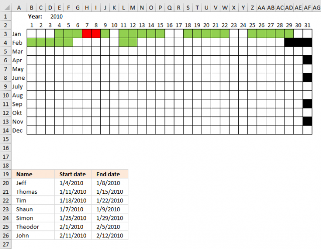
Plot date ranges in a calendar
The image above demonstrates cells highlighted using a conditional formatting formula based on a table containing date ranges. The calendar […]